Fuzzy Interactive Approach for a Multi-objective Supplier Selection
Problem under Robust Uncertainty
F. Khalili Goudarzi
1, A. Ghaffari
21. Department of Applied Mathematics, Shiraz University of Technology, Shiraz, I.R. Iran
2. Department of Electrical and Electronics Engineering, Shiraz University of Technology, Shiraz, I.R. Iran E-mail: [email protected];[email protected]
Received: 22 March 2020; Accepted: 14 May 2020; Available online: 15 June 2020
Abstract: In this paper, the authors proposed a multi-objective Mixed Integer Linear Programming (MILP) model for supplier selection problems. The main aim of the system under the investigation is to plan the companies to supply goods to achieve financial benefit by minimizing the total costs and satisfying the customers with on-time delivery and minimizing rejected items. In this case, some restrictions such as multi-product and multi-period conditions, shortage inventory constraints, and discount circumstances simultaneously are considered. Despite these efforts, due to the uncertainty nature of the problem, some parameters are considering as uncertainty data. For this aim, applying robust counterparts for uncertain parameters plays an essential role in real-world applications of this case. It is concluded that the feasibility and optimality properties of the usual solutions of real-world LPs can be severely affected by small changes of the data and that the robust optimization (RO) methodology can be successfully used to overcome this phenomenon.
Keywords: Supply selection; Supplier selection problem; Robust optimization; Robust counterpart (RO); Uncertain data.
1. Introduction
The reduction of production cost is one of the most essential critical for survival in the real world's competitive environment. Selecting the best suppliers as aparticularpart of a supply chain can effectively reduce the cost of purchasing and increase the competitiveness of the organizations and companies because, in most industries, the cost of raw materials of the product will contain most of the price of the product. Nowadays, supply chain management is an essential issue in the strategy of industrial companies and one of the most effective ways to create value for customers. The supply chain structure consists of potential suppliers, manufacturers, distributors, retailers, customers. Suppliers, as an essential member of the supply chain, have a vital role in achieving the objectives of a supply chain. The performance of the system can be improved by reducing costs by eliminating waste, continuous quality improvement to make zero defects rate, improving flexibility to satisfy the needs of final customers, reducing delays at various stages of the supply chain. The supplier selection problem is one of the most critical matters which affects the success of the supply chain, and many researchers pay attention to it in recent years; meanwhile, using the mathematic models is much accepted. One of the most significant business decisions faced by purchasing managers in a supply chain is the selection of appropriate suppliers while trying to satisfy multi-criteria based on price, quality, customer service, and delivery. Hence supplier selection is a multi-criteria decision-making problem that includes both qualitative and quantitative factors, some of which may conflict. In this problem, many criteria may conflict with each other, so the selection process becomes complicated and it contains two significant issues:
1) Which supplier(s) should be chosen?
2) How much should be purchased from each selected supplier?[1]
Sometimes suppliers offer quantity discounts to encourage companies and organizations towards larger orders. In this case, the buyer must decide what order quantities to assign to each supplier. In a real situation, for a supplier selection problem, most of the input information is not known precisely, since the decision-making deal with human judgment and comprehension and this might cause ambiguity in these problems. Deterministic models cannot easily take this vagueness into account. In these cases, the theory of robust optimization is one of the best tools to handle uncertainty. In this paper, the authors present a MILP model for a supplier selection problem and they are going to use robust optimization in order to counter with the vagueness of the data of the problem.
Researchers have traditionally addressed the problem of optimally controlling stochastic systems by taking a probabilistic view of randomness, where the uncertain variables are assumed to follow known probability
distributions and the goal is to minimize the expected cost or time. However, accurate probabilities are difficult to obtain in practice, in particular for distributions varying over time, and even small specification errors might change the optimality of the problem. Consequently, the optimal stochastic behavior might be numerically intractable, and even when available, it might be of limited practical communication if it was calculated with the wrong distribution.
The focus of robust optimization is to preserve the system against the worst-case value of the uncertainty in a predefined set. The term ‘‘robust optimization'' consists of several approaches for protecting the decision maker (DM) against parameter vagueness and stochastic uncertainty. At a high level, the manager must determine why he uses a robust solution: Is it a solution whose feasibility must be guaranteed for any realization of the uncertain parameters? Or whose distance to optimality must be guaranteed? The main paradigm relies on worst-case analysis: A solution is evaluated by using the realization of the uncertainty which is most unfavorable [2].
In the traditional linear optimization methodology, a small data uncertainty (even 1% or less) is not acceptable; the problem is solved as if the given ("nominal") data were accurate. In this case, small data uncertainties will not affect the feasibility and optimality properties of this solution significantly, or those small adjustments of the nominal solution will not affect the feasibility of the problem. But in real-world problems, these hopes are not necessarily justified, and sometimes even small data uncertainty has a considerable impact [3].
The structure of this paper is organized as follows: After introducing the problem and explaining some literature reviews, a multi-objective mixed-integer linear programming model for the supplier selection problem considering multi-product and multi-period conditions, shortage and inventory conditions, and considering discount circumstances is represented. Objectives in this problem are minimizing costs, minimizing rejected items, and maximizing on-time delivery. After that, the authors explain the RC of the problem and the ambiguous form of it. An interactive method is represented in order to solve the multi-objective problem. A numerical example is presented to illustrate the efficiency of the approach. Finally, a summary and conclusions are discussed.
2. Literature review
Supplier selection as one of the most critical issues in industry and management is a multi-criteria decision-making problem which contains both qualitative and quantitative objectives in conflict with each other. This issue is one of the most widely researched areas and has attracted the attention of many researchers. Multi-criteria supplier selection has been extensively studied in the literature since 1966, where Dickson [4] presented 23 criteria that have been considered by purchasing managers in various supplier selection problems. He had used 273 purchasing customers and representatives. Due to Dickson classified the significance placed on the mentioned 23 criteria, a nicely documented multi-objective nature of vendor selection had been obtained.
In 1991 Weber et al. [5] had made a comprehensive study on supplier selection decisions and its related technical concepts using the variety of different researches. The main aim of the mentioned study was to focus on criteria and analytical methods involved in the vendor selection process, and analyzing the influence of Just In Time (JIT) manufacturing strategies in this area. In order to categorize the related articles, 23 vendor selection criteria were considered and analyzed, which were based on a survey of purchasing customers and administrators. These twenty-three criteria were taken into consideration by Dickson.
Degraeve et al. [6] employed the Total Cost of Ownership (TCO) implication as an essential tool for analyzing different supplier selection models. In the mentioned study, TCO and all its related parameters overlook were discussed, which was used to represent the related assessments whenever the Cockerill Sambre ball is available. TCO determined all associated costs in the purchasing process throughout the whole fetter, the investigated company. In the mentioned study, different supplier selection methods are analyzed with the used data set by exploiting an advocated methodology. Then TCO analysis from supplier selection and inventory management models were considered by whom and when. Achieved results were compared with the solution that minimizes TCO. According to the mentioned study, it could be concluded employing multiple item mathematical programming models always yield better performance than single-item rating ones.
Stadtler [7] suggested a general quantity discount and supplier selection model. His proposed model considered not only the all-units discount but also the incremental discount case. Furthermore, the objective function chosen resolves (former) conflicts among proponents of a purely cost-oriented and cash flow oriented modeling approach. By considering the model formulation results in tight LP relaxations, near-optimal, and often optimal solutions had been generated with little computational efforts and less CPU time.
Moreover, just like in most real-world decision-making problems, uncertainty is another important property of supplier selection problems. Informational vagueness because of the tangible and intangible criteria of supplier selection problems must be taken into account to reach effective configuration and coordination of supply chains. A detailed classification and review of qualitative techniques for supply chain planning under uncertainty can be found in Peidro et al. [8] review paper.
Several methods have appeared in literature for supplier selection problem. Selim & Ozkarahan [9] modeled the SC distribution network. The goal of their model was to select the optimum numbers, locations, and capacity levels of plants and warehouses to deliver products to retailers at the least cost while satisfying the desired service level to retailers. The model distinguished itself from other models in this field in the modeling approach used. Because of the somewhat imprecise nature of retailers’ demands and decision-makers’ aspiration levels for the goals, a fuzzy modeling approach is used. Additionally, a novel and generic Interactive Fuzzy Goal Programming (IFGP)-based solution approach was proposed to determine the preferred compromise solution.
Wang and Yang [10] were investigated a novel fuzzy model in quantity discount environments to select the intended suppliers. The mentioned method reduced the complexity of the problem in comparison with traditional methods by avoiding to consider numerous heterogeneous criteria. Scaling and weighting problems had not been ignored in the mentioned study by exploiting Analytical Hierarchy Process (AHP) and fuzzy compromise programming. Due to the existence of conflicting criteria when different suppliers want to configure the best possible combination of purchasing quantities, the fundamental target function is considered as a multi-objective function. In order to define the related restrictions, supplier’s capacity and customer demands are taken into consideration. One of the main achievements in the mentioned study was simplifying the generation of a more objective compromise solution with the aid of fuzzy compromise programming and the generalized Multi-Objective Linear Programming (MOLP) model complexity of decision in purchasing situation was dramatically reduced.
Lee [11] suggested a fuzzy supplier selection model with the consideration of benefits, opportunities, costs, and risks. He considered a systematic approach to choose the best suppliers under a fuzzy environment. He also applied a fuzzy analytic hierarchy process (FAHP) model, which considered the benefits, opportunities, costs, and risks (BOCR) concepts to evaluate various features of suppliers. Multiple items which affected the performance of the relationship were analyzed by taking into account experts’ opinion on their efficiency, and a performance ranking of the suppliers was mentioned. To illustrate the effectiveness and practicality of his model, he applied a real-world case study of a TFT-LCD manufacturer in selecting the most appropriate BLU manufacturers. The proposed model was used to facilitate the decision process.
A comprehensive study on the issues of decision-making approaches for supplier selection was accomplished by William Ho et al. [12]. This research conducted extensive research and analyzed various decision-making models in order to make a satisfying analysis and conclusion. Studied models in this research included multi-criteria decision-making models and their effectiveness. In order to measure the effectiveness of multi-multi-criteria decision-making models, the study considered three essential concepts in the format of three questions. These questions were: 1- which models have been considered more useful and practical than the others? 2- Which kind of assessment has been investigated more to analyze decision-making approaches for supplier assessments? 3-does the researches in this area suffer from a lack of procedures? Trying to find an acceptable solution for these fundamental questions and comprehensive classification of the previous studies were presented in the mentioned study.
Chang et al. [13] suggested a fuzzy multi-choice goal programming for the supplier selection problem. They used Multi-Choice Goal Programming (MCGP) and fuzzy approaches by considering multiple aspiration levels and vague goal relations to find the best answer. They defined the membership function for each linguistic quantifier to describe their ambiguous selection preference in supplier selection. They applied a real-world case of a Liquid Crystal Display (LCD) monitor and acrylic sheet manufacturer to indicate the efficiency of their proposed method.
Kilincci & Onal [14] investigated a supplier selection problem for a famous washing machine company in Turkey. They used a fuzzy AHP based methodology to choose the best supplier with the most customer satisfaction. After defining the main three attributes and fourteen sub-attributes, which were determined based on the literature survey and the experience of the expert for supplier selection in order to design the hierarchy structure, the weights of attributes and sub-attributes and alternatives were calculated by using the fuzzy analytic hierarchy process approach.
Demirtas & Ustun [15] introduced new integrated models and their constraints, variables, and objectives. Then the solution methods of these integrated models were given. Finally, different integrated models were compared by considering their advantages and disadvantages.
Tahmasbi et al. [16] proposed a model based on the fact that the demand was uncertain and shortages were considered as lost sales. The buyer’s order lead time was a nonlinear function of the buyer’s order size and the number of shipments from the supplier. Quantity discount offers were used as a tool to achieve coordination between both parties.
Arikan [17] represented a fuzzy solution approach for multi-objective supplier selection. In his study, a multiple sourcing supplier selection problem was considered as a multi-objective LP problem. The objective functions of this research were minimization of costs, maximization of quality, and maximization of on-time delivery. He proposed a fuzzy mathematical model and a novel approach to satisfying the decision maker's aspirations for fuzzy
goals. His proposed method can practically use for non-dominated solutions. In order to indicate the efficiency of the proposed approach, a numerical example was considered. Demands for this problem was taken into consideration as fuzzy parameters and appropriate member function was applied for fuzzy data. His proposed model was ultimately the same as the known augmented max-min model except the additional constraints related to the decision-makers' preferred achievement levels. An ordinary and famous multi-objective supplier selection model was converted into convex fuzzy programming models with a single objective function. This conversion reduced the complexity of the problem resulting in less computational operations.
Beauchamp et al. [18] increased the performance of the Digital Manufacturing Market (DMM) by developing a column generation method for solving the supplier selection problem. The objective function of their proposed method was maximizing the technological competencies of the selected suppliers by considering the capacity constraints. Using the column generation procedure can also desirable to solve the problem of limited scalability of LP formulation and can be unified into the Digital Manufacturing Market. In this paper, the authors considered a supply chain problem considering multiple services that can be provided by multiple suppliers. This problem relates to a Multiple Sourcing Supplier Selection Problem (MSSSP). In this paper, three mathematical optimization models were suggested, which evaluated both operational and technological aspects such as suppliers’ technical competency, capacity, and geographic location, and manufacturers’ expected lead time for work orders.
Turk et al. [19] addressed an optimization problem by considering both supplier selection and inventory planning. The authors applied a two-stage approach to solve these problems. In the first stage, the rank of each supplier was calculated with different criteria such as cost, delivery, service, and product quality by using Interval Type-2 Fuzzy Sets (IT2FS)s. The inventory model was created in the following step. Then, by using a Multi-objective Evolutionary Algorithm (MOEA), conflicting Multi-objective functions of the problem were solved and optimal Pareto solutions were found. The authors evaluated the performance of three MOEAs with tuned parameter settings, namely NSGA-II, SPEA2, and IBEA, on a total of 24 synthetic and real-world instances. The numerical results indicated better performance of NSGA-II.
The supplier selection problem in the cardboard production process was taken into consideration by Niroomand et al. [20]. The Cardboard Company produced cardboard boxes in different sizes according to customer desire. The mentioned study focused on minimizing three essential subjects, including loss of raw material, cost of raw material, and excess production, which is useless. By considering an unpredictable cost and demand, a semi-real environment was considered in order to implement the proposed method. The mentioned model was formulated as multi-objective mixed-integer linear programming with uncertain demand and raw material price values, then the optimum solution was determined based on developing a weighted criterion approach and finding an optimal solution, namely Pareto. In order to consider different levels of uncertainty, Pareto optimal solution was employed using a variety of parameters and different weights.
3. Problem description
The system under investigation is composed of 𝑀𝑀 suppliers, 𝑁𝑁 items, 𝑘𝑘 price levels, and 𝑇𝑇 time periods. The basic aim of such a system is to select the optimal suppliers of the products in order to achieve some financial benefits and satisfying the customers with on-time delivery and less damage. Today, on-time delivery or on-time services are important for customers and companies. Delay in these issues not only affects the client but also reduces the credibility of companies or governments. In general, proper and accurate planning can greatly reduce associated costs, as well as reduce late-damages and minimize rejected items and thereby satisfy the customers with on-time delivery. In this case, some restrictions such as multi-product and multi-period conditions, shortage inventory constraints and discount circumstances simultaneously, etc. are considered.
3.1 Problem assumption
The following assumptions define the supplier selection problem of the above-explained system. 1) Multi-item can be purchased from each supplier.
2) Each supplier can supply multi-items.
3) The purchasing process considers as multi-period time, which can be monthly, yearly periods, etc. 4) The capacity of each supplier for any of the items is limited.
5) Shortage and inventory are allowed in every period except for the last one. 6) Quantity discounts in all periods and for all items are taken into consideration. 7) The demand for the items is constant and known with certainty.
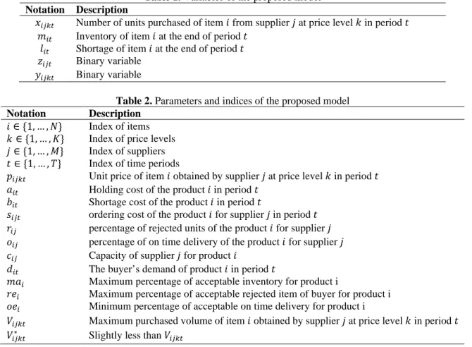
3.2 Notations
Under the above conditions, it is necessary to introduce the notations, including parameters, indices, and variables used in the proposed model. These notations are defined in Table 1-2.
Table 1. Variables of the proposed model
Notation Description
𝑥𝑥𝑖𝑖𝑖𝑖𝑖𝑖𝑖𝑖 Number of units purchased of item 𝑖𝑖 from supplier 𝑗𝑗 at price level 𝑘𝑘 in period 𝑡𝑡 𝑚𝑚𝑖𝑖𝑖𝑖 Inventory of item 𝑖𝑖 at the end of period 𝑡𝑡
𝑙𝑙𝑖𝑖𝑖𝑖 Shortage of item 𝑖𝑖 at the end of period 𝑡𝑡 𝑧𝑧𝑖𝑖𝑖𝑖𝑖𝑖 Binary variable
𝑦𝑦𝑖𝑖𝑖𝑖𝑖𝑖𝑖𝑖 Binary variable
Table 2. Parameters and indices of the proposed model
Notation Description
𝑖𝑖 ∈{1, … ,𝑁𝑁} Index of items
𝑘𝑘 ∈{1, … ,𝐾𝐾} Index of price levels
𝑗𝑗 ∈{1, … ,𝑀𝑀} Index of suppliers
𝑡𝑡 ∈{1, … ,𝑇𝑇} Index of time periods
𝑝𝑝𝑖𝑖𝑖𝑖𝑖𝑖𝑖𝑖 Unit price of item 𝑖𝑖 obtained by supplier 𝑗𝑗at price level 𝑘𝑘 in period 𝑡𝑡 𝑎𝑎𝑖𝑖𝑖𝑖 Holding cost of the product 𝑖𝑖 in period 𝑡𝑡
𝑏𝑏𝑖𝑖𝑖𝑖 Shortage cost of the product 𝑖𝑖 in period 𝑡𝑡
𝑠𝑠𝑖𝑖𝑖𝑖𝑖𝑖 ordering cost of the product 𝑖𝑖 for supplier 𝑗𝑗in period 𝑡𝑡 𝑟𝑟𝑖𝑖𝑖𝑖 percentage of rejected units of the product 𝑖𝑖 for supplier 𝑗𝑗 𝑜𝑜𝑖𝑖𝑖𝑖 percentage of on time delivery of the product 𝑖𝑖 for supplier 𝑗𝑗 𝑐𝑐𝑖𝑖𝑖𝑖 Capacity of supplier 𝑗𝑗 for product 𝑖𝑖
𝑑𝑑𝑖𝑖𝑖𝑖 The buyer’s demand of product 𝑖𝑖 in period 𝑡𝑡
𝑚𝑚𝑎𝑎𝑖𝑖 Maximum percentage of acceptable inventory for product i
𝑟𝑟𝑟𝑟𝑖𝑖 Maximum percentage of acceptable rejected item of buyer for product i 𝑜𝑜𝑟𝑟𝑖𝑖 Minimum percentage of acceptable on time delivery for product i
𝑉𝑉𝑖𝑖𝑖𝑖𝑖𝑖𝑖𝑖 Maximum purchased volume of item 𝑖𝑖 obtained by supplier 𝑗𝑗at price level 𝑘𝑘 in period 𝑡𝑡 𝑉𝑉𝑖𝑖𝑖𝑖𝑖𝑖𝑖𝑖∗ Slightly less than 𝑉𝑉𝑖𝑖𝑖𝑖𝑖𝑖𝑖𝑖
3.3 Mathematical model
After introducing the notations and the assumption of the problem, in this subsection, the mathematical model is formulated as follows: 𝑚𝑚𝑖𝑖𝑚𝑚 𝑍𝑍1=� � � � 𝑝𝑝𝑖𝑖𝑖𝑖𝑖𝑖𝑖𝑖𝑥𝑥𝑖𝑖𝑖𝑖𝑖𝑖𝑖𝑖 𝑇𝑇 𝑖𝑖=1 𝐾𝐾 𝑖𝑖=1 𝑀𝑀 𝑖𝑖=1 𝑁𝑁 𝑖𝑖=1 +� �(𝑎𝑎𝑖𝑖𝑖𝑖𝑚𝑚𝑖𝑖𝑖𝑖+𝑏𝑏𝑖𝑖𝑖𝑖𝑙𝑙𝑖𝑖𝑖𝑖) 𝑇𝑇 𝑖𝑖=1 𝑁𝑁 𝑖𝑖=1 +� � � 𝑠𝑠𝑖𝑖𝑖𝑖𝑖𝑖𝑧𝑧𝑖𝑖𝑖𝑖𝑖𝑖 𝑇𝑇 𝑖𝑖=1 𝑀𝑀 𝑖𝑖=1 𝑁𝑁 𝑖𝑖=1 (1) 𝑚𝑚𝑖𝑖𝑚𝑚 𝑍𝑍2=� � � � 𝑟𝑟𝑖𝑖𝑖𝑖𝑥𝑥𝑖𝑖𝑖𝑖𝑖𝑖𝑖𝑖 𝑇𝑇 𝑖𝑖=1 𝐾𝐾 𝑖𝑖=1 𝑀𝑀 𝑖𝑖=1 𝑁𝑁 𝑖𝑖=1 (2) 𝑚𝑚𝑎𝑎𝑥𝑥 𝑍𝑍3=� � � � 𝑜𝑜𝑖𝑖𝑖𝑖𝑥𝑥𝑖𝑖𝑖𝑖𝑖𝑖𝑖𝑖 𝑇𝑇 𝑖𝑖=1 𝐾𝐾 𝑖𝑖=1 𝑀𝑀 𝑖𝑖=1 𝑁𝑁 𝑖𝑖=1 (3) 𝑠𝑠.𝑡𝑡. � � 𝑥𝑥𝑖𝑖𝑖𝑖𝑖𝑖𝑖𝑖 𝑇𝑇 𝑖𝑖=1 ≤ 𝑐𝑐𝑖𝑖𝑖𝑖 𝐾𝐾 𝑖𝑖=1 ∀𝑖𝑖,𝑗𝑗 (4) � � 𝑥𝑥𝑖𝑖𝑖𝑖𝑖𝑖𝑖𝑖 𝐾𝐾 𝑖𝑖=1 𝑀𝑀 𝑖𝑖=1 =𝑑𝑑𝑖𝑖𝑖𝑖+𝑚𝑚𝑖𝑖𝑖𝑖− 𝑙𝑙𝑖𝑖𝑖𝑖 ∀𝑖𝑖,𝑡𝑡= 1 (5)
𝑚𝑚𝑖𝑖𝑖𝑖−1− 𝑙𝑙𝑖𝑖𝑖𝑖−1+� � 𝑥𝑥𝑖𝑖𝑖𝑖𝑖𝑖𝑖𝑖 𝐾𝐾 𝑖𝑖=1 𝑀𝑀 𝑖𝑖=1 =𝑑𝑑𝑖𝑖𝑖𝑖+𝑚𝑚𝑖𝑖𝑖𝑖− 𝑙𝑙𝑖𝑖𝑖𝑖 ∀𝑖𝑖,∀𝑡𝑡= 2, … , T−1 (6) 𝑚𝑚𝑖𝑖𝑖𝑖−1− 𝑙𝑙𝑖𝑖𝑖𝑖−1+� � 𝑥𝑥𝑖𝑖𝑖𝑖𝑖𝑖𝑖𝑖 𝐾𝐾 𝑖𝑖=1 𝑀𝑀 𝑖𝑖=1 =𝑑𝑑𝑖𝑖𝑖𝑖 ∀𝑖𝑖,𝑡𝑡=𝑇𝑇 (7) 𝑚𝑚𝑖𝑖𝑖𝑖≤ 𝑚𝑚𝑎𝑎𝑖𝑖 ∀𝑖𝑖,𝑡𝑡 (8) � � � 𝑟𝑟𝑖𝑖𝑖𝑖𝑥𝑥𝑖𝑖𝑖𝑖𝑖𝑖𝑖𝑖 𝑇𝑇 𝑖𝑖=1 𝐾𝐾 𝑖𝑖=1 𝑀𝑀 𝑖𝑖=1 ≤ � 𝑟𝑟𝑟𝑟𝑖𝑖𝑑𝑑𝑖𝑖𝑖𝑖 𝑇𝑇 𝑖𝑖=1 ∀𝑖𝑖 (9) � � ��1− 𝑜𝑜𝑖𝑖𝑖𝑖�𝑥𝑥𝑖𝑖𝑖𝑖𝑖𝑖𝑖𝑖 𝑇𝑇 𝑖𝑖=1 𝐾𝐾 𝑖𝑖=1 𝑀𝑀 𝑖𝑖=1 ≤ �(1− 𝑜𝑜𝑟𝑟𝑖𝑖)𝑑𝑑𝑖𝑖𝑖𝑖 𝑇𝑇 𝑖𝑖=1 ∀𝑖𝑖 (10) 𝑣𝑣𝑖𝑖𝑖𝑖𝑖𝑖−1𝑖𝑖𝑦𝑦𝑖𝑖𝑖𝑖𝑖𝑖𝑖𝑖≤ 𝑥𝑥𝑖𝑖𝑖𝑖𝑖𝑖𝑖𝑖 ∀𝑖𝑖,𝑗𝑗,𝑘𝑘,𝑡𝑡 (11) 𝑣𝑣𝑖𝑖𝑖𝑖𝑖𝑖−1𝑖𝑖𝑦𝑦𝑖𝑖𝑖𝑖𝑖𝑖𝑖𝑖≤ 𝑥𝑥𝑖𝑖𝑖𝑖𝑖𝑖𝑖𝑖 ∀𝑖𝑖,𝑗𝑗,𝑘𝑘,𝑡𝑡 (12) � 𝑦𝑦𝑖𝑖𝑖𝑖𝑖𝑖𝑖𝑖 𝐾𝐾 𝑖𝑖=1 =𝑧𝑧𝑖𝑖𝑖𝑖𝑖𝑖 ∀𝑖𝑖,𝑗𝑗,𝑡𝑡 (13) � 𝑥𝑥𝑖𝑖𝑖𝑖𝑖𝑖𝑖𝑖 𝐾𝐾 𝑖𝑖=1 ≤ 𝑀𝑀𝑧𝑧𝑖𝑖𝑖𝑖𝑖𝑖 ∀𝑖𝑖,𝑗𝑗,𝑡𝑡 (14) 𝑥𝑥𝑖𝑖𝑖𝑖𝑖𝑖𝑖𝑖≥0,𝑚𝑚𝑖𝑖𝑖𝑖,𝑙𝑙𝑖𝑖𝑖𝑖 ≥0,𝑦𝑦𝑖𝑖𝑖𝑖𝑖𝑖𝑖𝑖∈{0,1},𝑧𝑧𝑖𝑖𝑖𝑖𝑖𝑖∈{0,1} ∀𝑖𝑖,𝑗𝑗,𝑡𝑡 (15) In the above formulation, the objective function (1) minimizes all operational costs involving the costs of material, maintenance costs, the costs of the shortage of items, and the ordering costs. The objective function (2) minimizes the amount of waste (rejected items). The third goal of the problem is to maximize the number of items that are delivered on time. This aim is stated in (3). The set of constraints (4) state that the capacity of each supplier for any of items are limited and indicate that the amount of purchase of any product by any supplier cannot exceed the capacity of that supplier for the same product. Demand conditions are investigated in the constraints set (5)-(7). These constraints have been incorporated into this model due to their multi-periodicity and simultaneous consideration of shortage and inventory conditions. The maximum acceptable level of inventory for each item is defined in the constraints set (8). The constraints set (9) indicate the buyer's maximum acceptable level for the amount of rejected items purchased from each supplier. The constraints set (10) describes the minimum acceptable level of the buyer for on-time delivery. Clearly, suppliers with less on-time delivery levels than these ranges will not be selected. The model's discount conditions are described in (11) and (12). The constraints set (13) states that each supplier may be purchased at maximum one price level. The binary variable 𝑧𝑧𝑖𝑖𝑖𝑖𝑖𝑖 is applied in order to combine the cost of ordering multiple products in a single order for each supplier. This value is equal to one, if the buyer purchases 𝑖𝑖′s item from the supplier𝑗𝑗 in the period 𝑡𝑡, otherwise it is equal to zero. These integer variables are considered in the constraints set (14). The constraints set (15) describe nonnegative integer variables and binary variables of the problem, which illustrates the binary nature of the supplier selection problem.
4. Robust approach
Data uncertainty is a prominent aspect of many real-world problems. Sometimes ignoring uncertain data may lead to unacceptable solutions. In some cases, a small change will affect the feasibility or even optimality properties of the solution. In this study, the proposed Robust Counterpart (RC) of the uncertain problem is explained and implemented in our problem. The strategy will be as follows. First step is to restrict to uncertain problem with a certain objective. Then, the only required thing is a computationally tractable representation of the RC of a single uncertain linear constraint, that is, an equivalent representation of the RC by an exact system of efficiently verifiable convex inequalities. The RC of the problem is reformulated as the problem of minimizing the original objective under a small and finite system of explicit convex constraints [3]. Focusing one single uncertainty-affected linear inequality- a family
{𝑎𝑎𝑇𝑇𝑥𝑥 ≤ 𝑏𝑏}[
With data changing in the uncertainty set: 𝑢𝑢= {[𝑎𝑎;𝑏𝑏] = [𝑎𝑎0;𝑏𝑏0] +∑𝐿𝐿𝑙𝑙=1𝜁𝜁𝑙𝑙[𝑎𝑎𝑙𝑙;𝑏𝑏𝑙𝑙]:𝜁𝜁 ∈ 𝒵𝒵}, where, 𝒵𝒵 is a unit box and it is defined as follow:
𝒵𝒵=𝐵𝐵𝑜𝑜𝑥𝑥1≡{𝜁𝜁 ∈ ℝ𝐿𝐿: ‖𝜁𝜁‖∞≤1} (17) In this case, [𝑎𝑎0]𝑇𝑇𝑥𝑥+� 𝜁𝜁 𝑙𝑙[𝑎𝑎𝑙𝑙]𝑇𝑇𝑥𝑥 𝐿𝐿 𝑙𝑙=1 ≤ 𝑏𝑏0+� 𝜁𝜁 𝑙𝑙𝑏𝑏𝑙𝑙 𝐿𝐿 𝑙𝑙=1 ∀(𝜁𝜁:‖𝜁𝜁‖∞≤1) ⟺ � 𝜁𝜁𝑙𝑙[[𝑎𝑎𝑙𝑙]𝑇𝑇𝑥𝑥 − 𝑏𝑏𝑙𝑙]≤ 𝐿𝐿 𝑙𝑙=1 𝑏𝑏0−[𝑎𝑎0]𝑇𝑇𝑥𝑥 ∀(𝜁𝜁: |𝜁𝜁 𝑙𝑙|≤1,𝑙𝑙= 1, … ,𝐿𝐿) ⟺ [� 𝜁𝜁𝑙𝑙[[𝑎𝑎𝑙𝑙]𝑇𝑇𝑥𝑥 − 𝑏𝑏𝑙𝑙]]≤ 𝐿𝐿 𝑙𝑙=1 𝑏𝑏0−[𝑎𝑎0]𝑇𝑇𝑥𝑥 −1≤𝜁𝜁𝑚𝑚𝑎𝑎𝑚𝑚𝑙𝑙≤1 (18)
It is concluded that the tractable robust counterpart of this box as a system of linear inequalities convert as follow: � −𝑢𝑢𝑙𝑙≤[𝑎𝑎𝑙𝑙]𝑇𝑇𝑥𝑥 − 𝑏𝑏𝑙𝑙≤ 𝑢𝑢𝑙𝑙,𝑙𝑙= 1, … ,𝐿𝐿 [𝑎𝑎0]𝑇𝑇𝑥𝑥+� 𝑢𝑢 𝑙𝑙≤ 𝑏𝑏0 𝐿𝐿 𝑙𝑙=1 (19)
There are some uncertainty-affected “blocks” in the data, namely, the coefficients of constraints sets (4)-(9)-(10). The constraint (4), represents the limit of production capacity. The constraint (9) shows the maximum acceptable rate of buyer for rejected items. Constraint (10), describes the minimum acceptable rate of buyers for on-time delivery. The perturbation of the parameters for these constraints are unit box, as represented above in section 3.1. The uncertain parameters are 𝑐𝑐𝑖𝑖𝑖𝑖,𝑟𝑟𝑖𝑖𝑖𝑖,𝑟𝑟𝑟𝑟𝑖𝑖,𝑑𝑑𝑖𝑖𝑖𝑖,𝑜𝑜𝑖𝑖𝑖𝑖,𝑜𝑜𝑟𝑟𝑖𝑖. A candidate solution is thus robust feasible if and only if it satisfies the “worst” realization of all these constrains. The worst realization of these constrains is the one where the uncertain coefficients 𝑟𝑟𝑖𝑖𝑖𝑖,𝑜𝑜𝑟𝑟𝑖𝑖 are the set of their maximal value in the uncertain set and the uncertain coefficients 𝑐𝑐𝑖𝑖𝑖𝑖,𝑟𝑟𝑟𝑟𝑖𝑖,𝑑𝑑𝑖𝑖𝑖𝑖,𝑜𝑜𝑖𝑖𝑖𝑖 are the set of their minimal value in the uncertainty set.
5. Applying interactive fuzzy programming approach
In this paper, some previous interactive fuzzy approaches are investigated [21-26]. The structures of these interactive solution procedures are summarized in the following steps:
Step 1: Determine appropriate (computational tractable) robust counterpart for the imprecise parameters, as mention, above and formulate the original model for the problem.
Step 2: To obtain a satisfactory feasible solution, the positive ideal solution (PIS) and the negative ideal solution (NIS) are calculated for each objective function of the problem. The PIS value for each objective is obtained as follows: 𝑍𝑍𝑖𝑖𝑃𝑃𝑃𝑃𝑃𝑃=𝑀𝑀𝑖𝑖𝑚𝑚𝑍𝑍𝑖𝑖 s.t. 𝑣𝑣 ∈ 𝐹𝐹(𝑣𝑣) 𝑖𝑖= 1,2 (20) 𝑍𝑍3𝑃𝑃𝑃𝑃𝑃𝑃=𝑀𝑀𝑎𝑎𝑥𝑥𝑍𝑍3 s.t. 𝑣𝑣 ∈ 𝐹𝐹(𝑣𝑣) (21)
Where, F is the set of all constraints. To reduce the computational time, NIS can be estimate as follows. Let 𝑣𝑣ℎ∗ and 𝑍𝑍ℎ(𝑣𝑣ℎ∗) denote the decision vector associated with the PIS of h-𝑡𝑡ℎ objective function and the corresponding value of h-𝑡𝑡ℎ objective function, respectively. The NIS value for each objective is obtained as follows:
𝑍𝑍ℎ𝑁𝑁𝑃𝑃𝑃𝑃=𝑀𝑀𝑎𝑎𝑥𝑥𝑖𝑖=1,2{ 𝑍𝑍ℎ(𝜈𝜈𝑖𝑖∗)} s.t. 𝑣𝑣 ∈ 𝐹𝐹(𝑣𝑣) ℎ= 1,2 (22) 𝑍𝑍3𝑁𝑁𝑃𝑃𝑃𝑃=𝑀𝑀𝑎𝑎𝑥𝑥𝑖𝑖=1,2,3{ 𝑍𝑍3(𝜈𝜈𝑖𝑖∗)} s.t. 𝑣𝑣 ∈ 𝐹𝐹(𝑣𝑣) (23)
Step 3: Determine linear membership function for all objective functions according to the achieved values. These membership functions are as follows:
𝜇𝜇ℎ(𝑍𝑍ℎ) = ⎩ ⎪ ⎨ ⎪ ⎧1 𝑍𝑍ℎ≤ 𝑍𝑍ℎ𝑃𝑃𝑃𝑃𝑃𝑃 𝑍𝑍ℎ𝑁𝑁𝑃𝑃𝑃𝑃− 𝑍𝑍ℎ 𝑍𝑍ℎ𝑁𝑁𝑃𝑃𝑃𝑃− 𝑍𝑍 ℎ𝑃𝑃𝑃𝑃𝑃𝑃 𝑍𝑍ℎ 𝑃𝑃𝑃𝑃𝑃𝑃≤ 𝑍𝑍 ℎ ≤ 𝑍𝑍ℎ𝑁𝑁𝑃𝑃𝑃𝑃 0 𝑍𝑍ℎ≥ 𝑍𝑍ℎ𝑁𝑁𝑃𝑃𝑃𝑃 ℎ= 1,2 (24) 𝜇𝜇3(𝑍𝑍3) = ⎩ ⎪ ⎨ ⎪ ⎧1 𝑍𝑍3≥ 𝑍𝑍3𝑃𝑃𝑃𝑃𝑃𝑃 𝑍𝑍3− 𝑍𝑍ℎ𝑁𝑁𝑃𝑃𝑃𝑃 𝑍𝑍3𝑃𝑃𝑃𝑃𝑃𝑃− 𝑍𝑍3𝑁𝑁𝑃𝑃𝑃𝑃 𝑍𝑍ℎ3 𝑁𝑁𝑃𝑃𝑃𝑃≤ 𝑍𝑍 3≤ 𝑍𝑍3𝑃𝑃𝑃𝑃𝑃𝑃 0 𝑍𝑍ℎ≤ 𝑍𝑍3𝑁𝑁𝑃𝑃𝑃𝑃 (25)
Step 4: Convert the auxiliary MILP model into an equivalent single objective one by using the following methods:
1) LH method, as described before, is presented by Lai and Hwang [21]:
𝑚𝑚𝑎𝑎𝑥𝑥 𝜆𝜆(𝑥𝑥) =𝜆𝜆0+𝛿𝛿 � 𝜃𝜃𝑖𝑖𝜇𝜇𝑖𝑖(𝑍𝑍𝑖𝑖) 3 𝑖𝑖=1 s.t. Constraints (1)-(15). 𝜆𝜆0≤ 𝜇𝜇𝑖𝑖(𝑍𝑍𝑖𝑖) 𝑖𝑖= 1, . . ,3 0≤ 𝜆𝜆0≤1 (26)
Where 𝜆𝜆0 and 𝜇𝜇𝑖𝑖(𝑍𝑍𝑖𝑖) denote the minimum satisfaction degree of all objectives and the satisfaction degree of each objective, respectively. 𝜃𝜃𝑖𝑖 denotes the weight for the importance of 𝑖𝑖th objective, where ∑3𝑖𝑖=1𝜃𝜃𝑖𝑖= 1. These values are determined by decision-makers and 𝛿𝛿 is a small value as it is set to 0.01.
2) TH method, which is introduced by Torabi and Hassini [22]. In this paper, 𝛾𝛾 is set to 0.2. 𝑚𝑚𝑎𝑎𝑥𝑥 𝜆𝜆(𝑥𝑥) =𝛾𝛾𝜆𝜆0+ (1− 𝛾𝛾)� 𝜃𝜃𝑖𝑖𝜇𝜇𝑖𝑖(𝑍𝑍𝑖𝑖) 3 𝑖𝑖=1 s.t. Constraints (1)-(15). 𝜆𝜆0≤ 𝜇𝜇𝑖𝑖(𝑍𝑍𝑖𝑖) 𝑖𝑖= 1, . . ,3 0≤ 𝜆𝜆0≤1 (27)
3) MW method[23] is an extended version of Werners method [24]:
𝑚𝑚𝑎𝑎𝑥𝑥 𝜆𝜆(𝑥𝑥) =𝛾𝛾𝜆𝜆0+ (1− 𝛾𝛾)� 𝜃𝜃𝑖𝑖𝜆𝜆𝑖𝑖 3 𝑖𝑖=1
(28)
Constraints (1) and (15). 𝜆𝜆0+𝜆𝜆𝑖𝑖≤ 𝜇𝜇𝑖𝑖(𝑍𝑍𝑖𝑖) 𝑖𝑖= 1, . . ,3
0≤ 𝜆𝜆0≤1
In this case, the coefficient of compensation (𝛾𝛾) set 0.4 based on previous tests. This value controls the minimum satisfaction level of objectives as well as the compromise degree among the objective functions.
4) DY method, which is introduced by Demirli and Yimer [25]:
𝑚𝑚𝑎𝑎𝑥𝑥 𝜆𝜆 s.t. Constraints (1) and (15). 𝜃𝜃𝑖𝑖𝜆𝜆 ≤ 𝜇𝜇𝑖𝑖(𝑍𝑍𝑖𝑖) 𝑖𝑖= 1, . . ,3 0≤ 𝜆𝜆 ≤1 (29)
5) Niroomand method, which is presented by Niroomand et al. [26]:
𝑚𝑚𝑎𝑎𝑥𝑥 𝜆𝜆(𝑥𝑥) =𝛾𝛾𝜆𝜆0+ (1− 𝛾𝛾)� 𝜆𝜆𝑖𝑖 3 𝑖𝑖=1 s.t. Constraints (1) and (15). 𝜆𝜆0+𝜆𝜆𝑖𝑖≤ 𝜇𝜇𝑖𝑖(𝑍𝑍𝑖𝑖) 𝑖𝑖= 1, . . ,3 0≤ 𝜆𝜆0≤1 𝜆𝜆0≤ 𝜇𝜇𝑖𝑖(𝑥𝑥) (30)
Several fuzzy interactive programming methods exist in the literature. For more information see [1] and [27]-[32].
Step 5: Solve the proposed auxiliary crisp model by the MILP solver. If the decision maker is satisfied with this current efficient compromise solution, stop. Otherwise, provide another efficient solution by changing the value of some controllable parameters say 𝛾𝛾 and then go back to Step 3.
Step 6: After solving the problem, solutions must be put into the objective functions in order to find the best answer.
6. Numerical example
In order to evaluate the performance of these methods and analyze the proposed model, a numerical instance is applied. It is generated with uniform distribution consists of three suppliers, two price-levels, and three periods. All data are randomly generated. The parameters related to data of the problem, described in Table3. The maximum percentage of rejected items and the minimum percentage of acceptable on-time delivery are stated in Table 4. The demands of each product for each customer in each period are presented in Table 5. The ordering cost of the first and second products in all three periods are described in Table 6. The prices of first and second product units on the basis of the discount are shown in Tables 7 and 8, respectively. For evaluating the effect of any changes in the weight value for each objective function on the performance of these interactive methods, 11 different weights are taken into considerations and this value is selected from [0,1] interval and with 0.1 distance. This test problem is coded in AIMMS 3.12 software with CPLEX 12.4 solver and run on a computer with Intel® Core™ i7, 2.80 GHz processor.
Table 3. Data of the problem
third supplier second supplier First supplier product = 𝑖𝑖 Product 2 Product 1 Product 2 Product 1 Product 2 Product 1 supplier = 𝑗𝑗 [0.01,0.04] [0.02,0.05] [0.02,0.05] [0.01,0.05] [0.03,0.05] [0.03,0.05] 𝑟𝑟𝑖𝑖𝑖𝑖 [0.93,0.97] [0.85,0.91] [0.88,0.93] [0.95,0.99] [0.95,0.99] [0.97,0.99] 𝑜𝑜𝑖𝑖𝑖𝑖 [1700,1900] [1150,1250] [890,910] [890,910] [1150,1250] [750,825] 𝑐𝑐𝑖𝑖𝑖𝑖
Table 4. Maximum percentage of rejected units & the minimum percentage of acceptable on-time delivery Product 2 Product 1 [0.02,0.05] [0.01,0.04] 𝑟𝑟𝑟𝑟𝑖𝑖 [0.9,0.904] [0.924,0.930] 𝑜𝑜𝑟𝑟𝑖𝑖
Table 5. Demands of buyer Product 2 Product 1 supplier/product [999,1001] [595,605] First period [892,908] [390,400] second period [795,805] [498,502] third period
Table 6. Ordering cost of the first and second products.
Third period Second period First period supplier / period 550 550 550 First supplier 480 460 480 Second supplier 600 600 600 Third supplier
Table 7. Price of first products unit on the basis of the discount
<180 value of [85-180] value of [0,85] Period Supplier 14 14.5 15 First period First supplier 14 14.5 15 second period 14.5 15 16 third period <190 value of [95,190] value of [0,90] 16 16.5 17 First period Second supplier 16 16.5 17 second period 14.5 15 16 third period <1200 value of [120,200] Value of [0,120] 12 12.5 13 First period Third supplier 13 13.5 14 second period 13 13.5 14 third period
Table 8. Price of second products unit on the basis of the discount
< 150 value of [70,150] value of [0,70] Period Supplier 4 4.5 5 First period First supplier 4 4.5 5 second period 4.5 5 6 third period <160 value of [80,160] value of [0,80] 2 2.5 3 First period Second supplier 2 2.5 3 second period 2.5 3 4.5 third period <210 value of [125,210] value of [0,125] 6 6.5 7 First period Third Supplier 6 6.5 7 second period 7 7.5 8 third period
The holding cost and the shortage cost for all periods are the same and equal to 1 and 2, respectively. The maximum acceptable balance levels for the first and second products are equivalent to 400 and 800, respectively. The positive ideals answer of three objective functions are calculated. Now, by these positive ideal answers, negative ideal answers of each objective function are approximated by the use of the equations expressed in (22)-(23). These results are shown in Table 9.
Table 9. Positive ideal value (PIS) and the negative ideal answers of functions (NIS). 𝑍𝑍𝑖𝑖𝑁𝑁𝑃𝑃𝑃𝑃 𝑍𝑍𝑖𝑖𝑃𝑃𝑃𝑃𝑃𝑃 𝑖𝑖 48362 34155.5 𝑖𝑖=1 121 101.4175 𝑖𝑖=2 3930 4020.965 𝑖𝑖=3
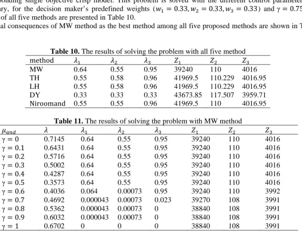
By applying the membership–functions and using fuzzy interactive methods the problem is changed to the corresponding single objective crisp model. This problem is solved with the different control parameters. In summary, for the decision maker’s predefined weights (𝑤𝑤1= 0.33,𝑤𝑤2= 0.33,𝑤𝑤3= 0.33) and γ= 0.75, the results of all five methods are presented in Table 10.
Fiscal consequences of MW method as the best method among all five proposed methods are shown in Table 11.
Table 10. The results of solving the problem with all five method
method 𝜆𝜆1 𝜆𝜆2 𝜆𝜆3 𝑍𝑍1 𝑍𝑍2 𝑍𝑍3 MW 0.64 0.55 0.95 39240 110 4016 TH 0.55 0.58 0.96 41969.5 110.229 4016.95 LH 0.55 0.58 0.96 41969.5 110.229 4016.95 DY 0.33 0.33 0.33 43673.85 117.507 3959.71 Niroomand 0.55 0.55 0.96 41969.5 110 4016.95
Table 11. The results of solving the problem with MW method
𝜇𝜇𝑎𝑎𝑎𝑎𝑎𝑎 𝜆𝜆 𝜆𝜆1 𝜆𝜆2 𝜆𝜆3 𝑍𝑍1 𝑍𝑍2 𝑍𝑍3 γ= 0 0.7145 0.64 0.55 0.95 39240 110 4016 γ= 0.1 0.6431 0.64 0.55 0.95 39240 110 4016 γ= 0.2 0.5716 0.64 0.55 0.95 39240 110 4016 γ= 0.3 0.5002 0.64 0.55 0.95 39240 110 4016 γ= 0.4 0.4287 0.64 0.55 0.95 39240 110 4016 γ= 0.5 0.3573 0.64 0.55 0.95 39240 110 4016 γ= 0.6 0.4036 0.064 0.00073 0.95 39240 110 3992 γ= 0.7 0.4692 0.000043 0.00073 0.023 39270 108 3991 γ= 0.8 0.5362 0.000043 0.00073 0 38840 108 3991 γ= 0.9 0.6032 0.000043 0.00073 0 38840 108 3991 γ= 1 0.6702 0 0 0 38840 108 3991
7. Conclusion
In this paper, a multi-objective mixed-integer linear programming (MOMILP) model is presented for supplier selection problem under the uncertainty conditions. Because several criteria affect the problem of supplier selection, the authors examined several non-parallel objectives simultaneously. This model consists of multi-product and multi-period conditions, shortage and inventory constraints, and discount conditions simultaneously. Due to the uncertainty nature of the problem, some parameters and constraints are considering as uncertainty data and uncertain constraints. In this case, computationally tractable robust counterparts of uncertain problems are explicitly obtained. Here we use box-RC in order to overcome uncertainty. This problem can help the DM to obtain the appropriate order to each supplier, and allows purchasing manager(s) to manage supply chain performance on service, quality, cost, etc.
The novelties in this program are considering some parameters as uncertain numbers which always govern the decision making processes, the multi-objective nature of the problem, and using five fuzzy interactive approaches in order to compare the results. The multi-objective formulation changed to the single objective form using fuzzy interactive programming approach. In order to find out the efficiency of these five methods, a problem instances were applied to demonstrate the application of the proposed methodology.
By focusing on the results of the test problem, it is obviously concluded that these fuzzy interactive methods are sensitive with respect to the change of minimum feasibility degree. Among these methods, the DY method has lower performance in comparison to other proposed methods. Although LH and TH methods approximately have the same performance, in some cases of these tables, TH has better performance than the LH method. Results obtained from the Niroomand method show it has better performance than LH and DY method, almost everywhere. Still, it is less sensitive to any change in importance degree of objectives than other methods and consequently, DM is less effective in decision making. Among all these five methods, the solutions obtained by the MW method have more balance in satisfaction degree of objectives and have less difference to the ideal values. Consequently, the results at the end show that while all methods perform reasonably well in both two test problems, MW acts better than others for both problem instances. This method is more appropriate and optimal for solving the supplier selection problem and it overcomes with uncertainty and prevents the optimality and feasibility with considering appropriate RC.
8. References
[1] Ozkok BA, Tiryaki F. A compensatory fuzzy approach to multi-objective linear supplier selection problem with multiple-item. Expert Systems with Applications. 2011; 38: 11363–11368.
[2] Gabrel V, Murat C, Thiele A. Recent advances in robust optimization: An overview. European Journal of Operational Research.2014; 235(3): 471-483.
[3] Ben-Tal A, El Ghaoui L, Nemirovski A. Robust optimization. Princeton University Press; 2009.
[4] Dickson GW. An analysis of supplier selection: systems and decisions. Journal of Purchasing. 1996; 201: 5– 17.
[5] Weber CA, Current JR, Benton WC. Vendor selection criteria and methods. European Journal of Operational Research. 1991; 50(1): 2-18.
[6] Degraeve Z, Labro E, Roodhooft F. An evaluation of supplier selection methods from a total cost of ownership perspective. European Journal of Operational Research. 2000; 125(1): 34–58.
[7] Stadtler H. A general quantity discount and supplier selection mixed integer programming model. OR Spectrum. 2006; 29(4): 723-744.
[8] Peidro D, Mula J, Poler R, Lario FC. Quantitative models for supply chain planning under uncertainty: a review. International Journal of Advanced Manufacturing Technology. 2009; 43: 400–420.
[9] Selim H, Ozkarahan I. A supply chain distribution network design model: an interactive fuzzy goal programming-based solution approach. The International Journal of Advanced Manufacturing Technology. 2008; 36: 401-418.
[10]Wang TY, Yang Y H. A fuzzy model for supplier selection in quantity discount environments. Expert Systems with Applications.2009; 36: 12179–12187.
[11]Lee AHI. A fuzzy supplier selection model with the consideration of benefits, opportunities, costs, and risks. Expert Systems with Applications. 2009; 36: 2879–2893.
[12]Ho W, Xu X, Dey PK. Multi-criteria decision making approaches for supplier evaluation and selection: A literature review. European Journal of Operational Research. 2010; 202(1): 16 – 24.
[13]Chang CT, Ku CY, Ho HP. Fuzzy multi-choice goal programming for supplier selection. International Journal of Operations Research and Information Systems. 2010; 1(3): 28-52.
[14]Kilincci O, Onal SA. Fuzzy AHP approach for supplier selection in a washing machine company. Expert Systems with Applications. 2011; 38: 9656–9664.
[15]Demirtas EA, Ustun O. Recent developments in supplier selection and order allocation process. Computer Engineering: Concepts, Methodologies, Tools and Applications. 2012; 5: 93-112.
[16]Tahmasbi H, Yu J, Sarker BR. An integrated production-supply system with uncertain demand, nonlinear lead time and allowable shortages. International Journal of Operations Research and Information Systems (IJORIS). 2012; 3(4): 1-18.
[17] Arikan F. A fuzzy solution approach for multi objective supplier selection. Expert Systems with Applications. 2013; 40: 947–952.
[18]Beauchamp H, Novoa C, Ameri F. Supplier selection and order allocation based on integer programming. International Journal of Operations Research and Information Systems (IJORIS). 2015; 6(3): 60-79.
[19]Turk S, Özcan E, John R. Multi-objective optimisation in inventory planning with supplier selection. Expert Systems with Applications. 2017; 78: 51-63.
[20]Niroomand S, Mosallaeipour S, Mahmoodirad A, Vizvari B. A study of a robust multi-objective supplier-material selection problem. IMA Journal of Management Mathematics. 2018; 29(3):325-349.
[21]Lai YJ, Hwang CL. A new approach to some possibilistic linear programming problems. Fuzzy Sets and Systems. 1992; 49(2): 121–133.
[22]Torabi ST, Hassini E. An interactive possibilistic programming approach for multiple objective supply chain master planning. Fuzzy Sets and Systems. 2008; 159: 193-214.
[23]Selim H, Ozkarahan I. A supply chain distribution network design model: An interactive fuzzy goal programming-based solution approach. The International Journal of Advanced Manufacturing Technology. 2008; 36(3-4): 401–418.
[24]Werners BM. Aggregation models in mathematical programming. Mathematical Models for Decision Support. 1988: 295–305.
[25]Demirli K, Yimer AD. Fuzzy scheduling of a build-to-order supply chain. International Journal of Production Research. 2008; 46(14): 3931–3958.
[26]Niroomand S, Mahmoodirad A, Mosallaeipour S. A hybrid solution approach for fuzzy multi objective dual supplier and material selection problem of carton box production systems. Expert Systems. 2019; 36(1): 1-17.
[27]Khalili Goodarzi F, Taghinezhad NA, Nasseri SH. A new fuzzy approach to solve a novel model of open shop scheduling problem. Scientific Bulletin: Series A. 2014; 76(3): 199-210.
[28]Khalili Goudarzi F, Nasseri SH, Taghinezhad NA. A new interactive approach for solving fully fuzzy mixed integer linear programming. Yugoslav Journal of Operations Research.2020; 30(1): 71-89.
[29]Alavidoost MH, Babazadeh H, Sayyari ST. An interactive fuzzy programming approach for bi-objective straight and U-shaped assembly line balancing problem. Applied Soft Computing. 2016; 40: 221–235. [30]Wu GH, Chang CK, Hsu LM. Comparisons of interactive fuzzy programming approaches for closed-loop
supply chain network design under uncertainty. Computers & Industrial Engineering. 2018; 125: 500-513. [31]Mari S, Memon M, Ramzan M, Qureshi S, Iqbal M. Interactive fuzzy multi criteria decision making approach
for supplier selection and order allocation in a resilient supply chain. Mathematics. 2019; 7(2): 137.
[32] Yildizbaşi A, Çalik A, Paksoy T, Farahani RZ, Weber GW. Multi-level optimization of an automotive
closed-loop supply chain network with interactive fuzzy programming approaches. Technological and Economic Development of Economy. 2019; 24(3): 1004-1028.
© 2020 by the author(s). This work is licensed under a Creative Commons Attribution 4.0 International License (http://creativecommons.org/licenses/by/4.0/). Authors retain copyright of their work, with first publication rights granted to Tech Reviews Ltd.
![Table 4. Maximum percentage of rejected units & the minimum percentage of acceptable on-time delivery Product 2 Product 1 [0.02,0.05] [0.01,0.04]](https://thumb-us.123doks.com/thumbv2/123dok_us/766018.2596890/10.892.118.769.125.971/maximum-percentage-rejected-percentage-acceptable-delivery-.webp)