Entropy-constrained scalar quantization with a lossy-compressed bit

Pradier,M.F., Olmos,P.M., Perez-Cruz,F.

(2016).Entropy-Constrained Scalar Quantization with a Lossy-Compressed

Bit.

Entropy

, 18(12), 449.

DOI:

https://doi.org/10.3390/e18120449

This work is licensed under a Creative Commons Attribution 4.0

International License

Entropy-Constrained Scalar Quantization with a

Lossy-Compressed Bit

Melanie F. Pradier1,2,*, Pablo M. Olmos1,2,* and Fernando Perez-Cruz1,3

1 _{Universidad Carlos III de Madrid, Madrid 28911, Spain}

2 _{Gregorio Marañón Health Research Institute, Madrid 28007, Spain}

3 _{Stevens Institute of Technology, Hoboken, NJ 07030, USA; [email protected]}

* Correspondence: [email protected] (M.F.P.); [email protected] (P.M.O.); Tel.: +34-916-246-005 (M.F.P.); +34-916-249-073 (P.M.O.)

Academic Editor: Raúl Alcaraz Martínez

Received: 8 September 2016; Accepted: 12 December 2016; Published: 16 December 2016

Abstract:We consider the compression of a continuous real-valued sourceXusing scalar quantizers and average squared error distortion D. Using lossless compression of the quantizer’s output, Gish and Pierce showed that uniform quantizing yields the smallest output entropy in the limit

D → 0, resulting in a rate penalty of 0.255 bits/sample above the Shannon Lower Bound (SLB). We present a scalar quantization scheme named lossy-bit entropy-constrained scalar quantization (Lb-ECSQ) that is able to reduce theD → 0 gap to SLB to 0.251 bits/sample by combining both lossless and binary lossy compression of the quantizer’s output. We also study the low-resolution regime and show that Lb-ECSQ significantly outperforms ECSQ in the case of 1-bit quantization.

Keywords:source coding; scalar quantization

1. Introduction

Entropy-constrained scalar quantization (ECSQ) is a well-known compression scheme where a scalar quantizerq(_·)is followed by a block lossless entropy-constrained encoder [1,2]. The two main quantities characterizing ECSQ are its distortion Dand rateR. For a real-valued input sourceX, the most common distortion measure is the mean squared error between the source X and its reconstruction ˆX. As the quantizerq(_·)is followed by entropy coding, the rateRis usually defined as the entropy of the random variable at the output of the quantizer, denoted byq(X).

A natural design problem is how to design q(_·) to achieve the lowest possible rate with distortion not greater thanD. While this problem can be solved numerically with various quantizer optimization algorithms [3–5], the expressions are only known whenXfollows an exponential [4] or uniform [6] distribution. The asymptotic limitD→0 constitutes an exception, as it is well known that an infinite-level uniform quantizer is optimal for a broad class of source distributions [1,7,8]. Further, asD→0, ECSQ with uniform quantizing is only 0.255 bits above Shannon’s lower bound (SLB) to the rate distortion functionR(D). SLB tends toR(D)asD→0, and is equal toR(D)for a Gaussian distributed source. Beyond scalar quantization,vector quantization(VQ) is the most common option to improve ECSQ; i.e., to achieve rates closer toR(D)at the same distortion level [9].

In this communication, we introduce a scalar quantization scheme that, in the limitD → 0, reduces the gap to Shannon’s lower bound to the rate distortion function R(D) to 0.251 bits. Furthermore, we show that in the low-resolution regime (1-bit quantization), the proposed scheme can remarkably improve ECSQ. The main idea of the proposed scheme is to encode the quantizer output by combining both lossless compression and binary lossy compression at a given Hamming distortion

DH, which offers an additional degree of freedom.

The compression scheme is straightforward, as we only need to expand ECSQ with an additional bit that encodes if the source symbol was in the left half or the right half of the quantization region that contained the source symbol. In other words, this scheme codes the least significant quantization bit lossily, allowing a certain Hamming distortionDH.

We refer to the proposed method as lossy-bit ECSQ (Lb-ECSQ). Note that Lb-ECSQ contains ECSQ as a particular solution, as ECSQ is recovered when the allowed distortion at the least significant quantization bit is set to zero.

The Lb-ECSQ method resembles works in the field of source-channel coding—namely, channel-optimized quantization [10]. Interestingly, when the output of a scalar quantizer is coded and transmitted via a very noisy channel, quantizers with a small number of levels (higher distortion) may yield better performance than those with a larger number of levels (lower distortion) [11]. Several works have addressed the design of scalar quantizers for noisy channels (e.g., [10–12]). All these works present conditions and algorithms to optimize the scalar quantizer given that it is followed by a noisy channel. This is similar to the Lb-ECSQ setup, where the lossy binary encoder behaves like a “noisy channel”, with an important and critical difference: in our problem, the distortion introduced by the lossy encoder (the“error probability” of the channel) is a parameter to be optimized, and acts as an additional degree of freedom. Note also that we solely consider the problem of source coding of a continuous source; encoded symbols are transmitted errorless to the receiver that aims at reconstructing the source.

We also study the low-resolution regime, in which we only encode the source with the lossy-bit—namely, 1-bit quantizer followed by a lossy entropy encoder. Results are distribution-dependent for the low-resolution regime, and we focus on the uniform and Gaussian distributions, which are interesting cases that show different behaviors. For example, in this low-resolution regime, the distortion can be reduced by 10% for a uniform distribution when we use 0.2 bits/sample.

In Section2of the paper, we review the analysis of ECSQ for an infinite-level uniform quantizer in the limitD→0. The asymptotic analysis of Lb-ECSQ for the same quantizer and same limit is presented in Section3. In Section4, we move to the opposite limit and compare both scalar quantization schemes with 1-bit quantizers.

2. ECSQ and the Uniform Quantizer

Suppose that a source produces the sequence of independent and identically distributed (i.i.d.) real-valued random variables {Xk,k ∈ Z} according to the distribution pX(x). A scalar quantizer is defined as a deterministic mapping q(·) from the source alphabet X ⊆ R to the

reconstruction alphabet ˆX, which is assumed to be countable. By Shannon’s source coding theorem,

q(X) can be losslessly described by a variable-length code whose expected length is roughly equal to its entropy H(q(X)). In ECSQ, this quantity constitutes the rate of the quantizer q(_·). Additionally, the mean squared-error distortion incurred by the scalar quantizerq(·)is given by

EX[(X−Xˆ)2], (1)

whereEXdenotes that the expectation is computed w.r.t. the source distributionpX(x). Consider the set of quantizersq(_·)for which the squared distortion in Equation (1) is smaller or equal toD∈R+,

and letRs(D)be the smallest rate achievable among this set; more precisely Rs(D),inf

q(·)H(q(X)) s.t. EX[(X−q(X))

2_{]≤D. (2)}

Under some constraints on the continuity and decay of pX(x), Gish and Pierce showed that in the limit D → 0, Rs(D) can asymptotically be achieved by the infinite-level uniform

quantizer, whose quantization regions partition the real line into intervals of equal lengths [1]. Further, they showed that

lim D→0{Rs(D)−R(D)}= 1 2log2 πe 6 , (3)

whereR(D)is the rate-distortion function of the source [13]. In the rest of this section, we briefly review the asymptotic analysis of ECSQ with uniform quantization following the approach described in [7,8]. We later rely on intermediate results to analyze the Lb-ECSQ scheme for the uniform quantizer. The following conditions are assumed for the source [7,8]:

C1 pX(x)logpX(x)is integrable, ensuring that the differential entropyh(X)is well-defined and finite; and

C2 the integer part of the sourceXhas finite entropy; i.e.,

H(_bXc)<∞ (4) otherwise,R(D)is infinite [14].

Denote the infinite-level uniform quantizer byqu(·), and letδbe the interval length. Forx∈R,

we have qu(x) =

∑

n n+1 2 δ1[nδ<x≤(n+1)δ], (5)

where (n+ 1₂)δis the reconstruction value for intervaln, and1[_·]denotes the indicator function. We define the piecewise-constant probability density function p(_Xδ)(x)as follows:

p(δ)

X (x) =

∑

n

pn

δ 1[nδ<x≤(n+1)δ], (6)

where pn , R_n(_δn+1)δpX(u)du is the probability that x belongs to that interval, and ∑npn = 1. To evaluate the squared error distortion, we first decomposeE[(X−qu(X))2]as follows:

EX[(X−qu(X))2] =∑n R(n+1)δ nδ x−(n+1₂)δ2pX(x)dx =∑_n pn δ R(n+1)δ nδ x−(n+1₂)δ2dx−∑n R(n+1)δ nδ pn δ −pX(x) x−(n+1₂)δ2dx. As shown in [7,8], the absolute value of the second term in the above equation can be upper-bounded byR p (δ) X (x)−pX(x)

dx, and this term vanishes asδ→0 according to Lebesgue’s

differentiation theorem and Scheffe’s lemma (Th. 16.12) [15]. Thus,

lim δ→0 EX[(X−qu(X))2] δ2 =δ −2

∑

n pn δ Z (n+1)δ nδ x−(n+1 2)δ 2 dx= 1 12. (7)

On the other hand, following [1], we express the entropy of the quantizer’s output H(qu(X))

as follows:

H(qu(X)) =

Z

p_X(δ)(x)log₂(p_X(δ)(x))dx−log₂(δ). (8) As shown in [16], the integral in the above expression converges toh(X)asδ→0, hence

whereo(1)refers to error terms that vanish asδtends to zero. We conclude that the uniform quantizer

qu(·)with quadratic distortionD=E[(X−qu(X))2]and rateRu(D),H(qu(X))achieves Ru(D) =h(X) +1 2log2 1 D− 1 2log2(12) +o(1) (10)

bits per sample, whereo(1)comprises error terms that vanish asDtends to zero. Further, for sources

Xsatisfying conditions C1 and C2, the rate-distortion functionR(D)can be approximated as [17]

R(D) =h(X) + 1 2log2( 1 D)− 1 2log2(2πe) +o(1). (11)

Without theo(1)term, the right-hand side (RHS) of Equation (11) is referred to theShannon lower bound(SLB). By combining Equations (10) and (11), we obtain

lim D→0{Ru(D)−R(D)}= 1 2log2(2πe)− 1 2log2(12)≈0.255 bits/sample (12)

3. Uniform Quantization with a Lossy-Compressed Bit

The above results show that—according to Equation (2)—uniform quantizers are asymptotically optimal as the allowed distortionDvanishes. In the following, we present a simple scheme that—while maintaining the scalar uniform quantizer—reduces the gap to the rate distortion function of the source below Equation (12). To this end, the quantizer’s output is compressed using both lossless and lossy compression, and thus the compression rate is no longer measured by the entropy of the quantizer’s output. Unlike in [1], we do not claim that uniform quantization is optimal according to the proposed definition of compression rate. Consider again the uniform quantizerqu(·)with interval lengthδ.

GivenXandqu(X), letb(X)be a binary random variable such that b(x) =

(

1, x≤qu(x)

0, x>qu(x)

. (13)

3.1. Compression with a Lossy-Compressed Bit

Given the random variable(qu(X),b(X)), we maintain the lossless variable-length encoder

to compressqu(X). Moreover, the binary random variableb(X)is lossy compressed with a certain

Hamming distortionDH, which is a free parameter to be tuned to minimize the squared error distortion. We refer to this compression scheme as ECSQ with a lossy-compressed bit (Lb-ECSQ).

We assume that lossy-compression ofb(X) at a Hamming distortion DH is optimally done, achieving the rate distortion function for a Bernoulli source with probability Pb , P(b(X) = 1). While this assumption is somewhat unrealistic, our main goal in this paper is to analyze the fundamental limits of the proposed scheme, as one would do in ECSQ when assuming that the scalar quantizer’s output is compressed at a rate equal to its entropy. For the actual implementation of Lb-ESCQ, practical schemes based on low-density generator-matrix (LDGM) [18] or lattice codes [19] could be investigated.

Under the assumption of optimal lossy binary compression, we define the Lb-ECSQ rate of the uniform quantizerqu(·)as

RLb-u(D,DH),H(qu(X)) +R(DH,Pb) =H(qu(X)) +h2(Pb)−h2(DH), (14) where with a slight abuse of notation we useR(DH,Pb)to denote the rate distortion function of a Bernoulli source with probabilityPb, andh2(·)is the binary entropy function. We are interested in

any source distributionpX(x)satisfying C1, then limδ→0Pb = 12. Using this result and Equation (9),

we have

RLb-u(D,DH) =h(X)−log2(δ) +1−h2(DH) +o(1), (15) whereo(1)comprises error terms that vanish asδtends to zero. Observe that if we takeDH = 0 (i.e., lossless compression is used for bothqu(X)andb(X)), in the limitδ→0 the rateR_Lb-ucoincides with the entropy of the uniform quantizer in Equation (9) with half the interval length—i.e.,δ0=δ/2.

3.2. Reconstruction Values and Squared Distortion with a Lossy-Compressed Bit

Since qu(X) is losslessly compressed, upon decompression, it is recovered with no error.

Let ˆb(X) be a binary random variable representing the reconstructed value forb(X). Due to the lossy compression at a certain Hamming distortion, there exists a non-zero reconstruction error; namely,P(bˆ(x)₆=b(x)_|X=x)>0 forDH>0. Given the pair(qu(X), ˆb(X)), we compute the source

reconstruction value ˆXas follows ˆ x=qu(x) + (1−2ˆb(x))c= ( (n+1₂)δ₋c bˆ(x) =1 (n+1₂)δ+c bˆ(x) =0 , (16) wherec ∈ [0,δ

2]is a parameter that—along withDH—will be optimized to minimize the squared

error distortion D = _{EX, ˆX}[(X−_Xˆ)2_{]. We note that the reconstruction rule in Equation (16) is}

possibly suboptimal.

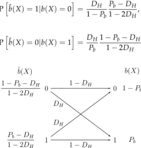
Before evaluatingDas a function ofδ,DH, andc, we first need to compute the error probabilities for theb(X)bit. Following [20] (Chapter 10), if(b(X), ˆb(X))are jointly distributed according to the binary symmetric channel shown in Figure1, then the mutual information I(b(X); ˆb(X))actually coincides with the Bernoulli rate distortion function R(DH,Pb) = h2(Pb)−h2(DH). Moreover, by using random coding in [20] (Chapter 10), it is shown that there exist encoding/decoding schemes that asymptotically (in the block-length) meet the input–output distribution in Figure1. Consequently, under the assumption of optimal lossy compression ofb(X)with prior probabilityPb, we can compute the error reconstruction probabilities by applying Bayes’ rule in Figure1,

Phbˆ(X) =1|b(X) =0i= DH 1−Pb Pb−DH 1−2DH, (17) Phbˆ(X) =0|b(X) =1i= DH Pb 1−Pb−DH 1−2DH . (18) ^_𝑏(𝑋) 0 1 𝑃𝑏−𝐷𝐻 1−2𝐷𝐻 1₋𝑃𝑏−𝐷𝐻 1−2𝐷𝐻 𝑏(𝑋) 𝑃𝑏 1₋𝑃𝑏 1−𝐷𝐻 1₋𝐷𝐻 𝐷𝐻 𝐷𝐻 0 1

Figure 1. Binary Source Channel model of the joint probability distribution between a Bernoulli sourceb(X)with prior probabilityPband its reconstruction ˆb(X)after lossy compression at Hamming

distortionDH, assuming that the Bernoulli rate distortion function is achieved.

Lemma 1. For any source X with a distribution pX(x)that satisfies conditions C1 and C2, lim δ→0 EX, ˆX[(X−Xˆ)2] δ2 = 1 48 1+12DH−12D2H (19)

under the assumption that the binary random variable b(X) defined in Equation (13) is optimally lossy compressed at a Hamming distortion DH.

Proof. Assuming optimal lossy compression, in the limitδ → 0, ˆb(X)is in error with probability

DH. Further, for anyδ>0, it is straightforward to check that both Equations (17) and (18) are upper bounded byDH. Therefore, the squared error distortion can be computed as follows:

EX, ˆX[(X−Xˆ)2]≤ Z

∑

ˆ x (x−xˆ)2p_Xˆ_|X=x(xˆ)pX(x)dx, (20) wherepXˆ|X=x(xˆ)is the conditional distribution of the reconstruction value forX=x, assuming that the reconstruction error probabilities are equal toDH. Equality is achieved atδ =0. According to Equation (16),p_Xˆ_|X=x(xˆ)can be expressed as follows: fornδ<x≤(n+1₂)δ, thenb(X) =1, and hence

pXˆ|X=x(xˆ) =      (1−DH) xˆ= (n+12)δ−c DH xˆ= (n+1₂)δ+c 0 otherwise (21)

and similarly, if(n+1₂)δ<x≤(n+1)δ, thenb(x) =0, and

p_Xˆ_|X=x(xˆ) =      (1−DH) xˆ= (n+12)δ+c DH xˆ= (n+12)δ−c 0 otherwise . (22)

As in Equation (7), we expand the integral in Equation (20) using the piecewise-constant distributionp(_Xδ)(x) EX, ˆX[(X−Xˆ)2]≤

∑

n pn δ Z (n+1)δ nδ

∑

_xˆ (x−xˆ)2pXˆ|X=x(xˆ)dx −

∑

n Z (n+1)δ nδ

∑

_xˆ hp_n δ −pX(x) i (x−xˆ)2p_Xˆ_|X=x(xˆ)dx, (23)

where it can be check that the absolute value of the second term is upper bounded by δ2R p (δ) X (x)−pX(x) dx, which vanishes asδ→0.

Using Equations (21) and (22), the first term in Equation (23) reads:

∑

n pn δ Z (n+1)_δ nδ

∑

_xˆ (x−xˆ)2pXˆ|X=x(xˆ)dx= δ2−6δr+12r2−DH(12δr−6δ2) 12 , (24) wherer= δ

2−c. The equality is obtained after straight-forward manipulation. The latter expression is

minimized if we chooser= δ

4(1+2DH), Equation (19) being the corresponding distortion. Note that

forDH=0, the reconstruction value is at the center of the interval,c=δ/4. Conversely, ifDH >0, the reconstruction point moves closer to the center of the next largest interval, such that the distortion caused by an erroneous transmission is reduced.

3.3. Asymptotic Gap to the Shannon Lower Bound

The following lemma jointly characterizes the rateRLb-uand squared distortionDof the Lb-ECSQ

scheme for the uniform quantizerqu(·)in the limitD→0:

Lemma 2. For any source X with a distribution pX(x)that satisfies conditions C1 and C2, the uniform quantizer

qu(·) with interval lengthδand Lb-ECSQ compression with quadratic distortion D = EX, ˆX[(X−Xˆ)2]and

Hamming distortion DHof the bit b(X)achieves

RLb-u(D,DH) =h(X) + 1 2log2 1 D− 1 2log2(12) +∆(DH) +o(1), (25)

where o(1)comprises error terms that vanish as D tends to zero, and ∆(DH) = 1

2log2(1+12DH−12D

2

H)−h2(DH). (26)

Proof. The proof is straightforward by combining Equations (15) and (19). More precisely, from Equation (19), we get that asδ→0, the following equality holds

δ= 48 EX, ˆX

[(X−_Xˆ₎2_]

(1+12DH−12D2H)

!1/2

. (27)

By plugging this equality into Equation (15), we get Equation (28), whereD=EX, ˆX[(X−Xˆ)2]. In Figure2, we plot∆(DH)forDH ∈ [0, 1/2]. Observe that∆(DH)is equal to zero atDH =0 andDH=1/2. However, for small values ofDH,∆(DH)is actually smaller than zero, achieving its minimum atD∗_H≈3.2×10−3_. 0 0.1 0.2 0.3 0.4 0.5 0 2 4 6 ×10−2 𝐷𝐻 Δ( 𝐷𝐻 ) 0 0.5 1 1.5 ×10−2 −6 −4 −20 2 4×10−3

Figure 2.∆(DH)function from Equation (26).

Corollary 1. The uniform quantizer qu(·)with interval lengthδand Lb-ECSQ compression with quadratic

distortion D=_E[(X−_Xˆ)2]achieves RLb-u(D,D∗H) =h(X) + 1 2log2 1 D− 1 2log2(12)−∆(D ∗ H) +o(1), (28) bits/sample, where∆(D∗_H)_≈0.004.

Finally, by combining Equations (11) and (28), lim D→0{RLb-u(D,D ∗ H)−R(D)}= 1 2log2(2πe)− 1 2log2(12)−∆(D∗H)≈0.251 (29)

bits/sample, which proves that Lb-ECSQ is able to outperform ECSQ in the limitD→0 using the uniform quantizerqu(·).

4. Lb-ECSQ in the High Distortion Regime

The above results demonstrate that the use of lossy compression can reduce the gap to SLB in the limitD → 0 with respect to ECSQ. Improvements can also be observed for low-to-moderate compression rates. The case of a quantizerq(_·)with only two quantization levels plays a special role that we analyze in this section. While the extension to an arbitrary numberNof quantization levels is interesting, preliminary results show that the biggest gain is achieved for a 2-level quantizer, and that the Lb-ECSQ performance tend withNvery quickly to the asymptotic gain(N→∞)described in the previous section. We consider a two-level quantizerq(_·)with quantization regionsA1={x :x≤α} andA2={x :x >α}for someα∈Rand two possible source distributions,X ∼U∈ [−δ/2,δ/2]

andX∼ N(0,σ2).

4.1. Two-Level Quantization of a Uniform Source

For the uniform sourceX∼U∈[₋δ/2,δ/2], the ECSQ rate is

Rq,H(q(X)) =h2(

α0

δ), (30)

where α0 = α+δ/2 andα ∈ [−δ/2,δ/2]. The squared distortion is minimized if reconstruction points are placed at the center of each quantization region [6]; i.e.,q(x) = α/2−δ/4 ifx ∈ A1and q(x) =α/2+δ/4 ifx∈ A2, and the distortion incurred is

EX[(X−q(X))2] = 1 δ α03 12 + (δ₋α03) 12 . (31)

In Figure3, we plotE[(X−q(X))2] vs. Rq as we vary α0 ∈ [0,δ] for δ = √12 (red curve with◦marker). As presented in Section3, Lb-ECSQ combines lossless compression ofq(X)with lossy compression of a random variableb(X)that gathers additional information of the sourceX

within the quantization region. As nowq(_·)only partitions the real line in two quantization regions, we implement Lb-ECSQ by directly lossy compressing the quantizer’s output q(X). To this end, we define the binary R.V.b(X) =1 ifx∈ A1and zero-otherwise. The Lb-ECSQ rate is given by the

compression rate ofb(X)at a certain Hamming distortionDH:

RLb-q ,h2(

α0

δ)−h2(DH). (32)

Further, we fix the quantizer threshold to α = 0, which implies that q(X) takes value either −δ

4 or δ4 with uniform probability, and thus RLb-q = 1−h2(DH). Under optimal lossy compression, the reconstructed bit ˆb(X)is in error with the same probability model described in Equations (17) and (18); namely, ˆb(X)is in error with probabilityDH. We set the source reconstruction

ˆ

X = ₋cif ˆb(X) = 1 and ˆX = cif ˆb(X) = 0, wherecis a positive quantity optimized to minimize

0.2 0.4 0.6 0.8 1 0 0.2 0.4 0.6 0.8 1

Squared error distortion𝐷

Rate

(bits/sample)

ECSQ

Lb-ECSQ(𝛼= 0)

Figure 3.Entropy-constrained scalar quantization (ECSQ) and lossy-bit ECSQ (Lb-ECSQ) rate distortion function for a 1-bit quantizer and uniform source,X∼U∈[₋δ/2,δ/2]forδ=√12.

Lemma 3. Given the source X ∼ U ∈ [₋δ/2,δ/2], the 1-bit quantizer q(_·) with threshold α = 0

and Lb-ECSQ compression achieves a squared distortion

EX, ˆX[(X−q(X))

2_{] =} δ2

48(1+12DH−12D

2

H) (33)

under the assumption that q(X)is optimally lossy compressed at a Hamming distortion DH.

Proof. The proof is similar to that of Lemma1, expandingE[(X−Xˆ)2]as done for every quantization

region done in and minimizing w.r.t. the reconstruction pointc.

In Figure3, we plotEX, ˆX[(X−Xˆ))2]in Equation (37) vs. RLb-q in Equation (32) forδ = √12 as we varyDH∈[0, 1/2](blue curve withmarker). Observe that Lb-ECSQ improves ECSQ at all points, except forDH =0 andDH =1/2, as we know they must be equivalent at these two points. The Lb-ECSQ analysis proposed forα=0 can be generalized to an arbitrary thresholdα∈[−δ/2,δ/2], but simulations forα6=0 using numerical optimization show that the obtained rate-distortion function coincides with the one computed forα=0. This result is dependent on the source distribution, as shown for the Gaussian source case.

4.2. Two-Level Quantization of a Gaussian Source

Now consider the same quantizerq(_·)andX∼ N(0,σ2). Low-resolution ECSQ for a Gaussian input source was studied in [21], where the authors showed that the minimum rate is achieved by a quantizer whose unique thresholdαgoes either to−∞or to∞asD→σ2, and the two reconstruction points are the centroids of the quantization regions. The ECSQ rate distortion function for this source is given by the following parametric curve

Rq =h2(Φ(α)), (34) EX[(X−q(X))2] = Z α −∞pX(x)(x−c1(α)) 2_dx+Z ∞ α pX(x)(x−c2(α))2dx, (35)

whereΦ(α)is the cumulative density function of the Gaussian distribution, and

c1(α) = 1 Φ(α) Z α −∞x pX(x)dx, c2(α) = 1 1−Φ(α) Z ∞ α x pX(x)dx. (36)

We now study the same Lb-ECSQ scheme analyzed before for the uniform source. First, we fix the quantizer threshold toα=0 and defineb(X) =1 ifX≤α, and zero otherwise. Note that Lb-ECSQ rate is given in Equation (32).

Lemma 4. Given the source X∼ N(0,σ2), the quantizer q(·)withα=0and Lb-ECSQ compression achieves

a squared distortion EX, ˆX[(X−Xˆ)2] = 1 σ − 2 σπ(1+4D 2 H−4DH) (37) for DH∈[0, 1/2].

Proof. The proof is based on expanding E[(X−Xˆ)2] as done for every quantization region in

Equation (24) and minimizing w.r.t. the reconstruction pointc.

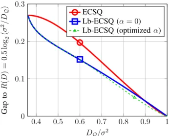
In Figure4, we plot the gap between the ECSQ and Lb-ECSQ rate distortion function for a 1-bit quantizer and the rate distortion function for the source; i.e.,R(D) =0.5 log₂(σ2/D). Observe that, unlike the case of a uniform source, forD/σ2→1, Lb-ECSQ is slightly worse than ECSQ. As discussed before, in the ECSQ solution for a Gaussian input source, the thresholdα goes to infinity in the limitD/σ2→1 [21]. By fixing the thresholdαto 0 in Lb-ECSQ, we are restraining to an equivalent solution. This can be tackled by generalizing the above equations to an arbitrary thresholdα. While the methodology is equivalent, we have to rely on numerical optimization to find the optimal choice ofα, c1(α), andc2(α)for each value of DH. In this case, the bit error reconstruction probabilities take the form given in Equations (17) and (18). Additionally, for an arbitrary thresholdα,b(X)is a Bernoulli source with probabilityp=Φ(α), and hence the compression rate isRLb-q =h2(p)−h2(DH). A numerical optimization (gradient descend) procedure has been used to find the minimum distortion for eachRLb-q. The results are shown in Figure4, where we can see that now Lb-ECSQ is able to

perform equally to or better than ECSQ in the whole range.

0

.

4

0

.

5

0

.

6

0

.

7

0

.

8

0

.

9

1

0

0

.

1

0

.

2

0

.

3

𝐷

_𝒬

/𝜎

2

Gap

to

𝑅

(

𝐷

)

=

0

.

5

log

2

(

𝜎

2

/𝐷

𝒬

)

ECSQ

Lb-ECSQ (

𝛼

= 0

)

Lb-ECSQ (optimized

𝛼

)

Figure 4.ForX∼ N(0,σ2), we plot the gap between the ECSQ and Lb-ECSQ rate distortion function

for a 1-bit quantizer and the rate distortion function for the source; i.e.,R(D) =0.5 log₂(σ2/D).

Acknowledgments: The authors wish to thank Tobias Koch and Gonzalo Vázquez Vilar for fruitful discussions and helpful comments to the manuscript. This work has been supported in part by the European Union 7th Framework Programme through the Marie Curie Initial Training Network “Machine Learning for Personalized Medicine” MLPM2012, Grant No. 316861, by the Spanish Ministry of Economy and Competitiveness and Ministry of Education under grants TEC2016-78434-C3-3-R (MINECO/FEDER, EU) and IJCI-2014-19150, and by Comunidad de Madrid (project ’CASI-CAM-CM’, id. S2013/ICE-2845).

Author Contributions:All authors have contributed equally to conceive and design the experiments, to analyze the data, and to write the paper. All authors have read and approved the final manuscript.

Conflicts of Interest:The authors declare no conflict of interest.

References

1. Gish, H.; Pierce, J. Asymptotically efficient quantizing.IEEE Trans. Inf. Theory1968,14, 676–683.

2. Goblick, T.; Holsinger, J. Analog source digitization: A comparison of theory and practice (Corresp.). IEEE Trans. Inf. Theory1967,13, 323–326.

3. Farvardin, N.; Modestino, J. Optimum quantizer performance for a class of non-Gaussian memoryless sources. IEEE Trans. Inf. Theory1984,30, 485–497.

4. Sullivan, G. Efficient scalar quantization of exponential and Laplacian random variables. IEEE Trans. Inf. Theory1996,42, 1365–1374.

5. Noll, P.; Zelinski, R. Bounds on Quantizer Performance in the Low Bit-Rate Region.IEEE Trans. Inf. Theory

1978,26, 300–304.

6. Gyorgy, A.; Linder, T. Optimal entropy-constrained scalar quantization of a uniform source. IEEE Trans. Inf. Theory2000,46, 2704–2711.

7. Linder, T.; Zeger, K. Asymptotic entropy-constrained performance of tessellating and universal randomized lattice quantization. IEEE Trans. Inf. Theory1994,40, 575–579.

8. Koch, T.; Vazquez-Vilar, G. Rate-Distortion Bounds for High-Resolution Vector Quantization via Gibbs’s Inequality.arxiv2015, arXiv:1507.08349.

9. Chou, P.A.; Lookabaugh, T.; Gray, R.M. Entropy-constrained vector quantization. IEEE Trans. Acoust. Speech Signal Process.1989,37, 31–42.

10. Farvardin, N.; Vaishampayan, V. Optimal quantizer design for noisy channels: An approach to combined source-channel coding. IEEE Trans. Inf. Theory1987,33, 827–838.

11. Spilker, J.J.Digital Communications by Satellite; Prentice-Hall: Upper Saddle River, NJ, USA, 1977. 12. Kurtenbach, A.J.; Wintz, P.A. Quantizing for noisy channels. IEEE Trans. Inf. Theory1969,17, 291–302. 13. Shannon, C.E. A mathematical theory of communication. Bell Syst. Tech. J.1948,27, 379–423.

14. Koch, T. The shannon lower bound is asymptotically tight for sources with finite renyi information dimension. IEEE Trans. Inf. Theory2015, doi:10.1109/TIT.2016.2604254.

15. Billingsley, P.Convergence of Probability Measures; John Wiley: New York, NY, USA, 1968.

16. Rényi, A. Probability Theory; North-Holland Series in Applied Mathematics and Mechanics; Elsevier: Budapest, Hungary, 1970.

17. Linder, T.; Zamir, R. On the asymptotic tightness of the Shannon lower bound. IEEE Trans. Inf. Theory1994, 40, 2026–2031.

18. Aref, V.; Macris, N.; Vuffray, M. Approaching the rate-distortion limit with spatial coupling, belief propagation, and decimation.IEEE Trans. Inf. Theory2015,61, 3954–3979.

19. Calderbank, A.R.; Fishburn, P.C.; Rabinovich, A. Covering properties of convolutional codes and associated lattices. IEEE Trans. Inf. Theory1995,41, 732–746.

20. Cover, T.M.; Thomas, J.A. Elements of Information Theory; Wiley Series in Telecommunications and Signal Processing; John Wiley & Sons, Inc.: Hoboken, NJ, USA, 2006.

21. Marco, D.; Neuhoff, D. Low-resolution scalar quantization for Gaussian sources and squared error. IEEE Trans. Inf. Theory2006,52, 1689–1697.

© 2016 by the authors; licensee MDPI, Basel, Switzerland. This article is an open access article distributed under the terms and conditions of the Creative Commons Attribution (CC-BY) license (http://creativecommons.org/licenses/by/4.0/).