Forecasting market returns: bagging or combining?

Forecasting Market Returns: Bagging or Combining?

Steven J. Jordan Econometric Solutions [email protected] Andrew Vivian Loughborough University [email protected] Mark E. Wohar

University of Nebraska-Omaha and Loughborough University [email protected]

May 17, 2016

Keywords: Return forecasting, Fundamentals, Macro variables, Technical indicators, Emerging

Forecasting Market Returns: Bagging or Combining?

Abstract

This paper provides a rigorous and detailed analysis of the methods of bagging, which addresses both

model and parameter uncertainty. We provide a multi-country study of bagging, of which there are very

few to date, that examines out-of-sample forecasts for the G7 and a broad set of Asian countries. We find

that, when portfolio weight restrictions are applied, bagging generally improves forecast accuracy and

generates economic gains relative to the benchmark. Bagging also performs well compared to forecast

combinations in this setting. We incorporate data mining critical values for appropriate inference on

bagging and combination forecast methods. We provide new evidence that the results for bagging cannot

be fully explained by data mining concerns. Finally, forecasting gains are highest for countries with high

trade openness and high FDI. The potentially substantial economic gains could well be operational given

1. INTRODUCTION

Most out-of-sample return forecasting evidence rests on major developed countries and is

especially focused on US data. The evidence generally suggests that it is difficult to consistently

outperform a simple benchmark. For example, Goyal and Welch (2003) state: “By assuming that the

equity premium was `like it always has been,’ a trader would have performed at least as well in most of

our samples.” The majority of the international literature considers several macro variables and

fundamental predictor variables based on dividends and earnings;1 it provides mixed evidence on the

extent of out-of-sample (OOS) predictability.2 However, there has been very little prior international

evidence on amalgamating information from these different predictor variables (Jordan and Vivian, 2011,

is a notable exception that considers one simple forecast combination technique). Our paper addresses

this topic in detail using the bagging method that explicitly accounts for model uncertainty and parameter

instability.

In the stock return context, given that predictive ability of individual variables is unstable, it is

important to control for model uncertainty and parameter instability (Bossaerts and Hillion, 1999; Paye

and Timmermann, 2006; Rapach and Wohar, 2006; amongst many others). According to Inoue and

Kilian, 2008 p511: “Bagging involves generating a large number of bootstrap resamples of the original

forecasting problem, applying a pretest model selection rule to each of the resamples, and averaging the

forecasts from the models selected by the pretest on each bootstrap sample.” Bagging explicitly accounts

for the model uncertainty by allowing the predictive model to change not only over time but also across

bootstrap samples for the same time period, by effectively averaging the parameter estimates across

bootstrap samples in each time period bagging addresses the parameter instability issue as well. Bagging

has recently been implemented for forecasting economic variables with applications to US inflation

1

Bossaerts and Hillion (1999) use fundamental predictors. Rapach, Wohar, and Rangvid (2005) examine macro predictors. Rapach and Wohar (2009) use the dividend-price ratio. Giot and Petitjean (2011) use fundamental predictors. Jordan and Vivian (2011) use fundamental predictors.

2

Jordan (2012) examines one particular type of time-variation in aggregate returns, long-term reversals. He finds these reversals can be explained by asset pricing models with time-varying risk factors and time-varying alphas; this suggests that macroeconomic factors are important determinants of time variation in equity returns.

(Inoue and Kilian, 2008) and US employment growth (Rapach and Strauss, 2010) but there is, to our

knowledge, very little empirical evidence on the effectiveness of bagging for a dataset of international

stock market returns nor in a multi-country setting more broadly.3

The main contribution of this paper is to provide a rigorous and detailed analysis of the bagging

method (Inoue and Kilian, 2008) for forecasting stock returns in Asia and the G7. The bagging method

has also been used for binary prediction problems where Lee and Yang (2006) considered an asymmetric

loss function with an application to forecasting the sign of the US stock market return. The branch of

bagging examined by Inoue and Kilian (2008) and followed in this paper applies to linear regression

models with continuous variables (predictors and predictand) where it is designed to reduce mean squared

forecast errors. Results of the bagging method relative to the no-predictability benchmark (a random-walk

with drift model) 4 _{are compared to the performance of forecast combination methods which have}

received little attention in stock return forecasting applications until recent studies of the US (Rapach,

Strauss and Zhou, 2010) and the G7 countries (Jordan and Vivian, 2011).5 _{We extend prior literature on}

bagging in important dimensions. Firstly, we incorporate data mining critical values for appropriate

inference on bagging (and combination forecast methods), which may be particularly important for the set

of G7 countries. Secondly, we estimate the utility gain that can be derived from bagging continuous

variables. Thirdly, we provide comprehensive evidence on bagging from 17 countries compared to prior

single country studies; this also enables us to examine cross-country determinants of forecast ability.

First, we examine whether or not data mining can account for the evidence of predictability that

we report? Prior literature focuses on the G7 applying bivariate regressions multiple times. Rapach and

Wohar (2006) demonstrate that data mining can partly account for evidence on aggregate return

3

Bagging was also implemented to estimate the appropriate restrictions on univariate US stock return predictability regressions by Hillebrand et al., (2013) but this setting is rather different to ours where we are using it in a multivariate predictive setting to tackle model uncertainty in an analogous way to Inoue and Kilian (2008) and Rapach and Strauss (2010).

4

We utilize an historical average benchmark to be consistent with prior literature. Robustness results using the AR(p) benchmark provide similar results to the historical average.

5

Forecast combination methods have been well established as effective in improving forecast accuracy in many disparate applications (Clemen, 1989), but perhaps surprisingly received little attention for stock returns until recently.

forecastability in the US. This suggests data mining could be a concern. The data mining issue is more

acute for the G7 countries as these countries have been investigated more often than the Asian countries.

Second, we investigate whether or not bagging generates utility gains in an asset allocation

exercise. Prior empirical investigations of bagging to US macroeconomic series do not examine the

economic value of bagging forecasts, while contemporaneous work does so in single country settings (e.g.

Jordan et al., 2016 for Canadian industries in terms of a sector rotation strategy). From a practical

perspective, our results suggest implementing equity index trading strategies based upon the new bagging

method in medium and smaller markets could help investors to time-vary their portfolio allocations

between debt and equity. Hence, we provide new evidence that bagging can generate economic value

which is robust to reasonable trading costs and cannot be fully accounted for by data mining concerns.

Third, we examine aggregate stock return forecasting for 11 Asian countries and the G7 (Japan is

in both groups) compared to prior international studies of equity market return predictability that

generally utilize a similar set of large economies consisting of the major developed countries.6 Major

developed countries stock returns are highly correlated with each other; for example in the G7 monthly

correlations are about 0.7 amongst country pairs. This suggests that data from these countries is only

partly independent from each other and may reflect one (or a small number of) common effect(s).7 In contrast, Asian financial markets have much lower correlations with each other and thus broaden

evidence compared to a sample exclusively of G7 countries. Moreover, Asian economies are of global

interest given that they produce about 30% of global economic output; make up over 40% of the world

population, are (generally) growing rapidly, and whose financial markets are emerging as an important

6

Bossaerts and Hillion (1999) use data from 1969-1995 for G7 and 7 other developed European countries. Rapach, Wohar, and Rangvid (2005) use data from mid 1970s to late 1990s for G7 and 5 other developed European countries. Rapach and Wohar (2009) study the G7 countries. Giot and Petitjean (2011) use data starting from early 1950s until 2005 for 10 developed countries. Jordan and Vivian (2011) use data from 1927-2009 for 7 developed countries. McMillan and Wohar (2011) use less sophisticated measures of economic value but include the G-7 countries and 4 Asian. Guidolin, Hyde, McMillan and Ono (2009) study the G-7.

7

Guidolin et al. (2009) find G7 countries return forecasting performance could be broadly split into two groups those that are Anglo-Saxon and those which are Continental European. Thus, results that hold for G7 markets may not transfer well to other markets and thus examining countries outside of Anglo-Saxon and Continental European warrants investigation.

investment class despite their higher volatility of stock returns and of economic fundamentals.8 Asian countries also differ in terms of economic, institutional, and cultural characteristics in comparison to the

US and other major developed countries.9 Forecast accuracy for a range of different predictands varies

across countries with differences in such characteristics (e.g. advanced versus developing countries,

Loungani, 2001; information disclosure and cultural traits, Bilinski et al., 2013; legal setting, Chen et al.,

2010), although rarely is the channel or mechanism through which this occurs formally outlined (notable

exceptions include Dovern et al., 2015; Loungani et al., 2013 who link forecast accuracy of professional

economists to information rigidities and efficient use of information). In terms of a stock return

application the characteristics outlined can impact the speed of the market response, e.g. market

development, information frictions and equity market liquidity should all impact how quickly news is

incorporated into stock prices.10 _{The greater the delay in reaction to news the more accurately the next}

periods return can be forecast. Whilst this area of analysis is at an early stage it still enables us to further

our understanding beyond that provided in prior analysis that considered alternative settings.11 _By

providing analysis on both Asian and G7 markets, we can provide comprehensive evidence on bagging

and whether country characteristics impact aggregate return forecastability across countries.

2. DATA DESCRIPTION

We examine two samples of countries: (1) the G7 countries for comparison to prior work and (2)

a subset of Asian countries for out-of-sample testing. Our eleven Asian countries include: China (CH),

8

Recent forecasting studies purely on Asia include Chen et al. (2012), Chen et al., (2016) and Qin et al. (2008) which have a multi-country focus, while single country studies include Chang et al. (2011) for Taiwan, Prskawetz et al. (2007) for India, Lewis-Beck and Tien (2012) for Japan and Wang et al. (2015) for China.

9

Compared to the G7 countries, our sample of Asian countries consist of firm that have: (1) smaller size, (2) higher B/M, and (3) more negative B/M firms. Culturally, our Asian sample of countries is more accepting of power inequalities and less individualistic than the G7 countries.

10

Theoretically, imperfect information models (Sims, 2003; Woodford, 2002) indicate there could be sluggish adjustment to indicator variables.

11

For example Jordan, Vivian and Wohar (2014b) provided some evidence on the cross-country variation in market return forecasts for European countries from bivariate predictive regressions (and a simple average combination). The current paper considers a larger number of countries, a broader set of factors and focuses on bagging but includes more while including a wider range of combination methods.

Hong Kong (HK), India (IN), Indonesia (ID), Japan (JP), Korea (KO), Malaysia (MY), Philippines (PH),

Singapore (SG), Thailand (TH) and Taiwan (TW), over a balanced sample period of 1995-2011

employing monthly data. The selection criteria are to include Central, East, South, and Southeast Asian

countries for which: (1) there is a Datastream (DS) Total Market Index and (2) there is data available

from at least 1995.12

The data is primarily from Thomson Datastream. We collect monthly data from January 1995 to

June 2011. The start date enables inclusion of a wide number of Asian countries for which there is

virtually no prior OOS forecasting evidence, with the exception of Japan.13 It also enables a reasonably

sized OOS test period. We have 96 monthly observations (some combination methods use 36

observations for optimization) before beginning the OOS forecasting period in 2003. G7 countries were

subsequently included at the suggestion of an Associate Editor. We obtain data for 10 predictor variables

including 8 of the variables used by Goyal and Welch (2008, hereafter GW).

We include the following fundamental variables from GW: i) Dividend–price ratio (log), (DP):

Difference between the log of dividends paid on the market index and the log of market index price,

where dividends are measured using a one-year moving sum, ii) Dividend yield (log), (DY): Difference

between the log of dividends and the log of one month lagged market index price, iii) Earnings–price ratio

(log), (EP): Difference between the log of earnings on the market index and the log of stock prices, where

earnings are measured using a one-year moving sum and iv) Book-to-market ratio, (BM): Ratio of book

value to market value for the market index.

We include the following two macroeconomic variables from GW: i) Risk-free rate, (RF): Interest

rate on a low risk short-term security and ii) Inflation, (INFL): Calculated from CPI; since inflation rate

data are generally released in the following month, we use one month lagged inflation data.

12 _{The following countries did not have a DS Total Market Index: Afghanistan, Bhutan, Brunei, Burma, Cambodia,} East Timor, Laos, Macau, Maldives, Mongolia, Nepal, Tajikstan, Turkmenistan, and Uzbekistan. For the following countries Market index data (not DS index) started after 1995: Bangladesh, Kazakhstan, and Vietnam. At the suggestion of a referee we excluded two small illiquid markets (Pakistan and Sri Lanka) and included Taiwan using alternative data from Datastream, such as the policy interest rate as a proxy for the risk-free rate.

13

In particular, there is very little prior OOS forecasting evidence on the economic value of return forecasts (portfolio allocation evidence) in our sample of countries, except for Japan.

We include the following two technical variables from GW: i) Stock variance, (SVAR): Sum of

squared weekly returns on the market index and ii) Net equity expansion, (NTIS): Ratio of twelve-month

moving sums of net issues by listed stocks to total market capitalization of index. We consider two new

variables in this context, which are also of interest to technical traders: i) Price Pressure, (PRES):

Calculated as the ratio of the number of rising stocks in the previous month divided by the number of

falling stocks and ii) Change in Volume, (CVm): Calculated as the monthly change in the volume of

traded stocks (in the index).

Table 1 provides a summary of descriptive statistics for our sample countries. We report the

mean and the standard deviation for each independent variable used and for the aggregate market return.

There are several interesting comparisons. First, the average nominal returns (RET) vary substantially

across countries from -0.0015 (-0.15% per month or -1.8% per year compounded) in Japan, up to 0.0111

(1.11% per month or 14.2% per year compounded) in Indonesia. The standard deviation of returns also

varies substantially across countries from 0.0422 for the UK to 0.1048 for China. This means the Sharpe

ratio (return per unit of risk) varies dramatically across countries from over 0.09 in the US to a negative

-0.029 in the Philippines. The wide variation across countries exists for most of the variables we study.

[INSERT TABLE 1 AROUND HERE]

Table 2 contains the correlation matrix for returns across our sample countries. There is

substantial difference in correlation between the different country pairs. Interestingly the

cross-correlations in Asian countries’ returns are modest, on average about 0.40; the lowest correlation is

between China and Indonesia at 0.195. This is interesting since the G7 developed markets typically used

in prior literature tend to have correlations above 0.70 on average; this is important since G7 studies may

be capturing just a single (or small number) of common effect(s).

3. METHODOLOGY

3.A. Assessing the Impact of Individual Variables

Individual predictive regression models are used to estimate the linkage between the dependent,

lagged dependent, and a potential predictor variable (including its lags). Define ΔRIt = RIt− RIt−1, where

RIt is the log-level of the total stock return index (stock price index that includes reinvested dividends) at

month t.14 In addition, define y_{t t h}h_,+ =

(

1 /h

)

∑

h_j=1∆RI_t+j so that

y

_{t t h}h_,+ is the (approximate) monthly growth rate of the stock return index from time t to t + h, where h is the forecast horizon. In this section

we outline the general models for h step ahead forecasts, however in the empirical analysis we purely

focus on 1 step ahead forecasts (h=1). These predictive regression models take the form of (1) below:

,+

= +

α λ

,

+

ε

+

h h

t t h i t t h

y

x

(1)

This model can be employed to estimate h-step ahead forecasts of stock returns using a recursive

expanding window.

y

_{t t h}h_,+ , is linear in the potential predictor variables (i.e., Xt). The parameter α is a

constant. The parameter λ capture the effect of the potential predictor variable. Finally,

ε

_th_+h is an error term. For each country’s stock return, 10 regression models are estimated one for each of the 10

explanatory variables.

The models generated are used to conduct 1 step-ahead out-of-sample forecasts of stock returns.

These forecasts are then compared to the respective benchmark model, which takes the form of the

historical average (a random walk with drift model). The form of the benchmark model is the same as in

(1) where all the λj’s = 0.

14

3.B. Assessing the Impact of Variable Groups

3.B.1. Forecast Combinations

The method of forecast combining is considered to be a useful technique for "...sharing strengths

of different forecasting procedures..." (Yang, 2004:205) and is an alternative method of imposing

"...structure on high-dimensional forecasting models" (Stock and Watson, 2004:1). Empirical as well as

theoretical evidence (see Clemen and Winkler, 1986; Rapach and Strauss, 2010; Stock and Watson, 2003;

2004; and Yang, 2004) indicates that forecast combining generally improves the predictive ability of

models because it includes more variables or potential predictors, thus increasing the amount of

information used in generating forecasts. Recent work by Rapach, Strauss and Zhou (2010) demonstrates

combination forecasts are also useful for US stock index returns. The forecast combination methods used

in this paper include mean, median, trimmed mean, Discounted Mean Squared Forecast Errors (MSFE),

and Cluster (C), and Principal Components (PC) combinations. According to Rapach and Strauss (2008,

2010), these combination methods can be described below in (2):

∑

= + + = n i h t | h t, i t, i h t | h t, CB w ˆy y ˆ 1 (2)

where

y

ˆ

CBh ,t+h|t is the combined forecast of the variable of interest from individual regression models (1)

and wi,t is the weight of the individual regression forecasts,

h t | h , t, i y

ˆ _{+ is the individual forecast. The weights}

sum to unity.

It is now well known that combining forecasts generally improves OOS forecast performance in a

wide range of applications including aggregate financial variables. Hence, we discuss each method

intuitively and refer the reader to Rapach and Strauss (2010) for full details of its estimation. We

investigate a total of eight combination methods from four different types. Firstly, three simple

combination strategies are examined: Mean, Median, and the Trimmed mean, where the trim excludes the

lowest and highest forecasts from the average. Second, we use two discount forecast combination

Stock and Watson (2004), we use use δ = 1.0 (no discounting of past forecasts) and δ = 0.9 (more weight on most recent forecasts) resulting in Stock and Watson's discounted mean-square forecast error

(DMSFE) methods DMSFE(1) and DMSFE(0.9). Thirdly, we use cluster combinations to control for

forecast persistence (see Aiolfi and Timmermann, 2006). Utilizing a hold-out period, the individual

ARDL models are ranked by their mean square forecast error (MSFE) and clusters are created by

consecutively adding the next lowest MSFE ARDL model to the cluster. Clusters are formed on the

MSFE over a rolling window. Within the cluster with previous best (PB) MSFE an average of ARDL

model forecasts are taken to generate the cluster combination forecast. We utilize this method with two

clusters [C(2,PB)] and three clusters [C(3,PB)].15 _{Finally, we apply a principal component method to the}

individual ARDL model forecasts. We estimate the number of components with the ICp3 criterion up to

a maximum of 4 (Bai and Ng, 2002). See Stock and Watson (2004) for further details. We label this final

combination method as PC(C,3B).

3.C. Construction of Bagging Forecasts

Recall that

y

_{t t h}h_,+ is the monthly stock return from time t to t + h, where h is the forecast horizon.

Let xi,t denote one of n potential predictors of stock returns (so that i = 1, . . ., n). We consider 10 potential

predictors of stock returns (n = 10) in our analysis.

We compute bagging forecasts of stock returns at horizon h using the bagging-augmented

pretesting procedure (BA) of Inoue and Kilian (2008). The procedure begins with the general model:

, , 1

,

n h h t t h i i t t h i

y

₊

µ

δ

x

x

₊ =

= +

∑

+

(3)

where

x

_th_+h is an error term characterized by autocorrelation of degree h − 1. Suppose we are interested in

forming a forecast of

y

_th_+h at time t . The pretesting procedure involves estimating (3) via ordinary least

15

squares (OLS) using data from the start of the available sample through time t and computing the

t-statistics corresponding to each of the potential predictors.16 The xi,t variables with t-statistics less than

1.645 in absolute value are dropped from (3), and the model is estimated a second time using only

significant predictors.

Bagging can be implemented for the pretesting procedure via a moving-block bootstrap. More

specifically, a large number (B) of pseudo samples of size t for the left-hand-side and right-hand-side

variables in (5) are generated by randomly drawing blocks of size m (with replacement) from the

observations of these variables available from the beginning of the sample through time t. For each

pseudo-sample, we estimate (5) using the pseudo-data and OLS, the (pretesting) procedure determines the

predictors to include in the forecasting model, the model is re-estimated using the pseudo-data, and a

forecast of

y

_th_+h is formed by plugging the actual included xi,t values into the re-estimated version of the

forecasting model (and again setting the error term equal to its expected value of zero). The bagging

model forecast corresponds to the average of the B forecasts for the bootstrapped pseudo samples.17

Dividing the complete available sample of T observations for Δyt and xi,t (i = 1, . . . , n) into an

in-sample portion comprised of the first R observations and an out-of-in-sample period comprised of the last P

observations, we can form a series of P − (h − 1) recursive simulated out-of-sample forecasts using the bagging procedure.18 We denote this series by

{

y

ˆ

}

T h

.

R t h t | h t, BA − = + 3.D. Statistical Tests

Tests for encompassing and equal forecast accuracy

In the case of nested models, Clark and McCracken (2001) and McCracken (2007) develop a set

of asymptotics that allow for an out-of-sample test of equal population-level predictive ability between

16_{The t -statistics for the OLS estimates of δ}

i in (5) are computed using Newey and West (1987) heteroscedasticity and autocorrelation consistent (HAC) standard errors based on a lag truncation of h − 1.

17

Following Inoue and Kilian (2008), we use m = h. We use B = 1000. 18

“

two nested models. They show that, in the context of linear, OLS-estimated models, a number of different

statistics can be employed to test for equal forecast accuracy and forecast encompassing, despite the fact

that the models are nested. Based on Monte Carlo simulations, Clark and McCracken (2001, 2004)

indicate that ENC–NEW is the most powerful statistic, followed by their ENC-t,MSE – F and the MSE –

T statistics. These rankings suggest that the forecast encompassing statistics, especially ENC – NEW, can

have important power advantages over test statistics based on relative MSFE. We report results for the

most powerful statistic ENC-NEW, which is an F type test and is related to the Harvey et al. (1998)

statistic designed to test for forecast encompassing. It has been shown through extensive Monte Carlo

simulations in Clark and McCracken (2001, 2004) that the ENC-NEW statistic has power

advantages over the original Diebold and Mariano (1995) statistic as well as the Harvey et al. (1998)

ENC-t statistic which applies to nested forecasting models.

Under the null hypothesis, the restricted model forecasts encompass the unrestricted model

forecasts, while under the one-sided (upper-tail) alternative hypothesis the restricted model forecasts do

not encompass the unrestricted model forecasts. Clark and McCracken (2001) note that the limiting

distribution of the ENC-NEW statistic is non-standard and pivotal for one step ahead forecasts (h

= 1) considered in this paper. Clark and McCracken (2004) recommend basing inferences the ENC –

NEW statistics on a bootstrap procedure, given that the statistics are not in general asymptotically pivotal

(when h>1). The bootstrap procedure we employ is similar to the one in Clark and McCracken (2004),

which is a version of the Kilian (1999) bootstrap procedure, and is discussed in detail in Rapach and

Weber (2004) and Rapach and Wohar (2006).

Clark and West (2006, 2007) demonstrate that the ENC-t test can be viewed as an adjusted test

for equal MSE. In the Clark and West framework the null hypothesis is a random walk and the alternative

hypothesis is of a predictive regression. If the null hypothesis of a random walk is true then it will have a

lower mean-squared error relative to the alternative (despite the fact the alternative include an additional

variable) due to the fact that there is sampling error associated with estimating the alternative model. The

error. The CW-t statistic proposed by Clark and West (2006, 2007) is equivalent to the Harvey et al.

(1998) ENC-t test for forecast encompassing as considered in such studies as Clark and McCracken

(2001, 2005).

3.E. Measuring Economic Value

Our final set of empirical tests deal with the economic value of forecasts. We analyze if portfolio

allocations could have been improved by following the regression model rather than the historical average

benchmark. We consider a mean-variance optimizing investor. We take the return forecast from the

historical average benchmark and compare it to an alternative return forecast from i) bagging and ii)

combination forecast methods.

Recall that

y

_t+1is the log stock return. Define Yt+1 as the stock return (Yt+1 = exp(yt+1)-1. A

mean-variance optimizing investor has objective function:

2

1

2 2

(

)

(

)

2

p

2

p

2

p

p Y p y y

O

=

E Y

−

γ

σ

≈

E y

+

σ

−

γ

σ

(4)

where O is the objective, Yp is the portfolio return,

y

_pis the portfolio log return, and

γ

is the coefficient

of relative risk aversion. Such an investor will choose a portfolio weight,

ω

_{t b,}

( )

ω

_{t z,} of the risky asset under the prediction from the historical average benchmark (the alternative forecast model [bagging or

forecast combination]):19 1, , ₂

(

)

1

t b f t b t

E Y

Y

ω

γ

σ

+



−



 

=

 







 



(5) 1, , ₂

(

)

1

t z f t z t

E Y

Y

ω

γ

σ

+



−



 

=

 







 



(6)

19

Yf is the risk-free rate. We use 5-year rolling monthly data to estimate volatility

( )

2 t

σ

; however,

estimating volatility using alternative horizons has very little impact on the utility gain since

σ

_t2 is the

same in the benchmark weight,

ω

_{t b,} , and the alternative model weight placed,

ω

_{t z,} (see the denominator in equations 12 and 13 above).

The utility gain (

∆

O

) from using the regression model rather than the historical average benchmark is:

(

2 2

)

2 z b z b Y Y O Y Y

γ σ σ

∆ = − − − (7)

Second, we implement Goetzmann et al.’s (2007) performance measure (referred to as GISW):

1 1 1 1 1, 1, 1, 1, 0 0

1

1

1

1

1

ln

ln

1

1

1

ln[ (1

)] ln(1

)

where: =

Var[ln(1

)]

T T t z t b t f t f t t m f m

Y

Y

GISW

T

Y

T

Y

E

Y

Y

Y

−G −G − − + + + + = =







+









+



















=















−















− G



+





+



















+

−

+

G

+

∑

∑

(8)

GISW measures the average performance of a portfolio relative to the risk-free rate; it is a certainty

equivalent measure of abnormal performance. The parameter Gis set to reflect the overall reward (return) to risk (variance) ratio for each country based upon our sample data. This reduces the possibility

of manipulation and incorrect inference.

3.F. Data Mining Robust Critical Values

When testing the predictive ability of a large number of financial variables, Lo and MacKinlay

(1990) and Inoue and Kilian (2005) note that data mining is a serious concern when one is dealing with

stock return predictability regardless of whether the tests are in-sample or out-out-sample. Inoue and

Kilian (2005) note that an important way in which data mining can be controlled for is to use appropriate

critical values, which explicitly account for the possibility of data mining. Here we employ the data mining

predictive regressions, we focus on combinations and bagging in this paper. We calculate the two

out-of-sample statistics (MSE-F and CW-t) and the economic value measures for all models (each of the forecast

combination techniques and bagging) in turn. For each pseudo sample we store the maximal values for

each metric. We repeat this (whole) process 5000 times, to generate an empirical distribution for each of

the maximal out-of-sample statistics and for each of the maximal economic value measures. After

ordering the empirical distribution for each maximal statistic, the 4,500th, 4,750th, and 4,950th values

serve as the 10%, 5%, and 1% critical values for each maximal statistic.

4. OUT-OF-SAMPLE STOCK RETURN FORECASTS

Could investors’ actually utilize fundamental-price based models in order to benefit from more

accurate predictions of future stock returns? This issue is of importance to both practitioners and

academics alike. Asset managers, economic policymakers, as well as pension providers and contributors

all need accurate estimates of future market returns.

In this section, we examine a range of fundamental-price ratios as well as macro and technical

variables for a sample of Asian countries. Following Rapach, Strauss, and Zhou (2010) and Stock and

Watson (2004) we consider if various combining forecasts or bagging methods can improve forecast

accuracy over individual models. The historical average model is used as the benchmark.

4.A OOS Forecast Accuracy (Individual Regression Forecasts)

Table 3 shows 1-month forecast results for individual predictive regression models.20

Overall, the

individual predictive models have mixed results. In the Asian markets, some predictors provide dismal

forecasts, such as stock variance (SVAR), net equity issuance (NTIS), and change in volume at the

monthly frequency (CVM). However, the performance of individual fundamental-price ratios, e.g.,

dividend-price ratio (DP), dividend yield (DY), earnings price (EP), and book-to-market (BM), with the

20

exception of EP, show evidence of predictability. DP, DY, and BM show predictability above that of the

benchmark model in 8 of 11 countries. We implement the Clark and McCracken (2001) ENC-NEW

encompassing test and the Clark and West (2007) CW-T test of equal forecast accuracy. Predictability in

our Asian sample is robust even if very high hurdles associated with data snooping adjustments are made,

however data-snooping significance in fundamentals is found only under the ENC-NEW. Technical

indicators, e.g., price pressure as measured by rising stocks against falling stocks (PRES), also

demonstrate some predictability. PRES demonstrates predictability in 6 of 11 countries using standard

statistical significance tests and in 2 of 11 countries after adjusting for data-snooping bias. The risk-free

rate (RF) and inflation (INFL) are the only two predictors that demonstrate predictability under both the

CW-T test and data-snooping bias adjustments. Thus, it appears that investors interested in Asian

markets should specifically consider these variables in forecasting models.

[INSERT TABLE 3 AROUND HERE]

Predictability in the G7 countries is not found to be robust in our tests. Fundamental ratios do not

perform well in the G7 sample. The lack of robust statistical evidence of predictability in the G7 countries

contrasts sharply with the robust predictability found in our sample of Asian countries. The evidence for

predictability in G7 countries is even more dismal once data mining adjustments are made. When data

mining adjustments are used, there is virtually no evidence of predictability in the G7 countries.

There is also considerable variation in predictability across countries. Although there is virtually

no predictability in the G7, there is evidence at the 5% significance level for DE (Germany), JP, and the

US. In the Asian sample, we find there is no evidence of OOS predictability in China as no variable

demonstrates predictability when data-snooping bias is controlled. Predictability is also weak for the

other large Asian markets (HK, India, Japan, Korea, and Taiwan) where out of 10 predictor variables only

one exhibits some predictability after data-snooping bias adjustments. However, four countries

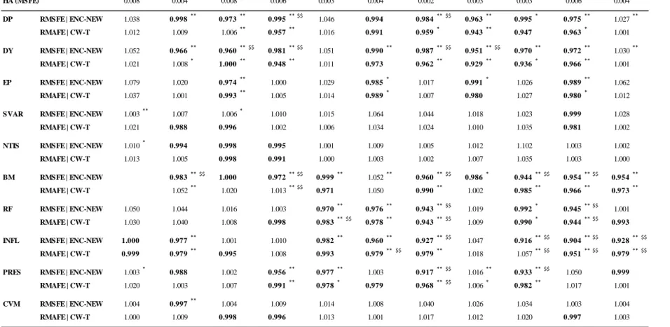
4.B OOS Forecast Accuracy (Bagging and forecast combinations)

This section contains the forecast results from bagging and forecast combinations. Table 4

reports results for the 1-month forecast horizon. We find consistent evidence in our Asian sample that

combining forecasts improves forecast accuracy in our sample of Asian countries even after adjustments

are made for data-snooping bias. This is true for seven of eight methods examined, the lone exception is

the principal component method (PC(C,3B)), and in 10 of 11 countries there are consistent improvements

in forecast accuracy, the sole exception is China. The lack of predictability in China may be due to

structural reforms in its equity market that substantially increase the proportion of tradable shares after

2005, which is near the start of our forecasting period (see Li et al., 2011 for further information on the

impact of this reform). Combination forecasts provide consistently large gains in HK, India, Indonesia,

Malaysia, Singapore, and Thailand. The finding that combination forecasts consistently perform well is

strengthened by the fact they are subject to greater parameter estimation error than the benchmark.

Clark-West (2007) emphasize that parameter estimation error leads to an expectation that the mean-squared

prediction error from an alternative model (here the forecast combination) is larger than that from a

parsimonious model (here the benchmark).

[INSERT TABLE 4 AROUND HERE]

Once more, in the G7 set of countries the results for predictability is not promising. There is little

to no evidence with predictability only documented for JP and the US for combination methods and only

for JP for bagging methods. Again, this is in complete contrast to the results found for Asia.

We note that the various classes of forecast combination methods yield broadly similar results;

hence in the subsequent analysis we only report results from one method in each class: Mean, DMSFE(1),

C(2,PB) and PC(C,3B); we can confirm results from the other combination techniques in the subsequent

tests are qualitatively similar to those of the same combination class that is reported.

In terms of forecast errors, the bagging method provides mixed results for the majority of Asian

countries; in general it underperforms the benchmark. For several countries (China, HK, Korea,

substantial magnitude. However, bagging does provide substantial improvement for four countries:

Indonesia, Japan, Malaysia, and Thailand. These results for bagging are in contrast to prior literature that

provides favorable results for the bagging method when applied to macroeconomic forecasts (Inoue and

Kilian, 2008; Rapach and Strauss, 2010).

6. ECONOMIC SIGNIFICANCE OF STOCK RETURN FORECASTS

6.A Economic Gains (Bagging and Combination Forecasts)

Table 5 and Table 6 present the results for the bagging method and various combination methods

for economic gains. Tables 5 and 6 provide results for the utility gain method and the manipulation proof

method, respectively.

The utility gain method for bagging indicates large outperformance of the benchmark is available

in several Asian countries, including HK, ID, KO, SG, TH, and TW. For Singapore, annualized gains in

utility of more than 10 percentage points across most models are possible. For other countries gains are

more modest, but still economically large, e.g., one can easily gain more than 5 percentage points in HK,

ID, and MY. For the average forecast combinations (AV COMB), utility gains are generally about 1 to 10

percentage points for 9 of the 11 countries. In the G7 countries, modest utility gains are generally

available. However, more than 5% can be realized in DE, FR, and the UK. The evidence suggests that

bagging performance is robust to data mining adjustments.

Economic gains with combination forecasts exist for China. Overall, combination methods

consistently provide economic value across countries and these results are robust to data snooping bias in

the Asian sample of countries. Before data bias adjustments, almost every combination model performs

well across our sample of countries. After data snooping bias adjustments evidence of predictability

weakens substantially; the most consistently performing method is the cluster approach PC(3,PB) with

economic gains in only 4 of 11 markets. So far, the results are broadly consistent with the statistical test

results in Table 4. The major difference between Table 4 and Table 5 is that bagging demonstrates large

and 15.63% in TW. We report gains when relative risk aversion is 3, i.e., P(UG), and when relative risk

aversion is 5 , i.e., P(UG5). The results are consistent for both values.

The bagging method can generate value for investors in G7 markets and this is statistically

significant in most markets except the US and Canada. The statistical evidence for bagging is most

consistent for Germany and France although Japan and UK also have some support that gains are

significant using the approach we implement to address data mining concerns. In terms of the

combination methods, the results are generally, quite similar to those for bagging. Positive gains can be

earned in most countries; however, these are typically smaller than those from the bagging method and

statistical evidence of outperformance largely evaporates when measures to adjust for data mining are

implemented.

[INSERT Table 5 AROUND HERE]

Table 6 provides results for a manipulation proof measure of economic gain. The GISW certainty

equivalent gains confirm the conclusions drawn from Table 5. For the G7, the GISW results are much

larger than under the utility gain measure. Overall, GISW gains can be large both in Asian countries (e.g.,

14.62 for the mean combination in SG) and exist across almost all countries.21 _{Again, bagging is a}

reliable model for attaining economic gains. After the manipulation proof adjustments, bagging

outperforms the benchmark in every country and does so at a significant level in 6 of the 11 Asian

countries and in 4 of the 7 G7 countries. Unlike the combination models, gains are available by using the

bagging method even after controlling for data snooping bias. As in Table 5, we report gains when

relative risk aversion is 3, i.e., GISW, and when relative risk aversion is 5, i.e., GISW5. The results are

again broadly consistent for both values of risk aversion.

[INSERT Table 6 and 7 AROUND HERE]

21

In some countries, e.g., TH, the risk-return tradeoff is negative, meaning that the risk-free rate is higher than the average stock return. This will affect the manipulation-proof measure since it looks at the return on the model relative to the risk-free rate. Then it takes this to the power of 1-risk-return tradeoff. But in the case of Thailand this is negative, so this inverts the relationship, which will drive the undesirable negative result. So a caveat to using the manipulation proof method is that one must be careful to ensure there is a positive equity premium; if not, then one should interpret the method’s results cautiously.

In Table 7 we examine the impact of accounting for trading costs on the utility gain measure. We

report results for trading costs of 10 basis points (on the portion of the portfolio adjusted), although

results are qualitatively similar if 30 basis points are used or if the GISW measure is implemented. The

results in Table 7 are very similar to Table 5. In fact, generally the net impact on economic value is less

than 0.2% p.a. It should be noted that re-balancing costs are incurred by the historical average allocations

as well, but even if these are assumed to be zero, the impact of transaction costs is not large because the

average change in portfolio allocation per period is small.

The most striking part of the economic value results (in Tables 5-7) is that for bagging these are

in clear contrast to those under the forecast accuracy approach (see Table 4). In contrast to its poor

forecast accuracy performance, bagging performs well in economic tests across countries and usually is a

top or comparable performer when compared to the combination predictor results. We shall explore

reasons for this difference in Tables 8. Overall, the economic value results are consistent for both the

utility gain and the manipulation proof measure methods, with the prior results slightly stronger. For the

G7 especially, both bagging and forecast combination methods provide more consistent evidence of

economic gains than of forecast accuracy.

6.B Discussion and Further Exploration

Section 6.A demonstrates that both bagging and combination forecasts would enable an investor

to tilt their portfolio to increase utility and to make certainty equivalent gains. Simply, when the

regression model predicts high (low) returns, the portfolio is tilted towards equities (T-bills). Our

empirical results suggest there is some economic value from forecasting returns with macro and technical

variables that could potentially be exploited by practitioners. Our results also indicate that noise may be

an issue and that consistent results are best obtained with a combination of many forecasts or by

simulating the relationship utilizing in-sample data.

The economic value results differ from forecast accuracy results. A possible reason for this is that

squared error rule; however, in the economic value exercise a restriction on portfolio weight ameliorates

the impact of large forecast errors. The results for bagging were different when we conducted economic

value tests (performed well) compared to forecast accuracy measures (performed poorly). The economic

value tests employ a restriction that the portfolio weight is between 0 and 1.5. The forecast accuracy tests

do not have such a portfolio weight restriction. In Table 8, we explore whether the bagging method

performed poorly in the forecast accuracy tests due to lack of restrictions. The restricted model (here

winsorization of extreme forecasts) will reduce the variance of the forecast compared to the unrestricted

model and if it moves the unrestricted model 'closer' to the true model will generate gains in forecasting

by reducing forecast error. Thus, we apply equivalent restrictions on the forecast accuracy tests as we did

in the economic value tests. We require that the forecast return must be between the risk-free rate (Yf)

and 1.5 times the risk aversion coefficient (

γ

)

times the variance of the return (

σ

_t2

)

plus the risk-free rate (Yf): 2 1,

(

)

1.5( )

f t b f t

Y

≤

E Y

₊

≤

Y

+

γ σ

.

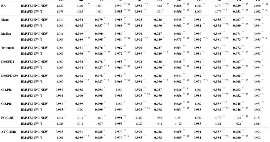
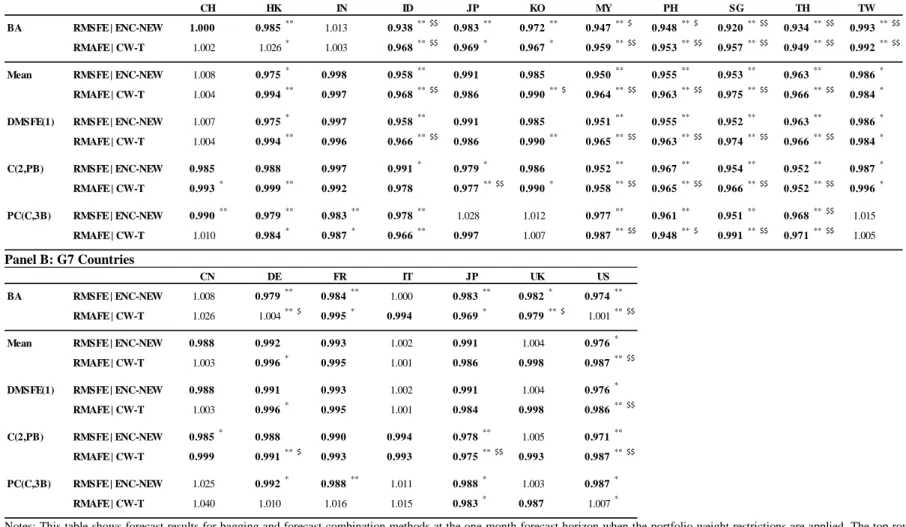
We rerun the forecast accuracy tests of Table 4 with these restrictions imposed, which are

reported in Table 8. For the Asian subset of countries the results with restrictions applied are given in

Panel A of Table 8. Almost every single model outperforms the benchmark for more than one-half of the

countries, with many methods doing considerably better when restrictions apply. Bagging now performs

strongly and the performance is very robust to data mining bias. The average combination forecasts

generally perform better and are more robust to data mining bias. Our results of this table indicate that

applying restrictions on the forecast return may be an important improvement to forecast performance

tests in Asian markets. This finding is consistent with the restricted model being 'closer' to the true model

than the unrestricted model since in this case gains in forecasting occur due to reduced estimation error of

the forecast. The lack of restrictions on Bagging in our initial forecast accuracy tests (Table 4) are thus an

important factor for the differing results between the accuracy tests and the economic gain tests (Tables

Panel B of Table 8 also provides some evidence that the bagging procedure can beat the

benchmark in 5 (4) of the G7 countries using the RMSFE (RMAFE) measure. There is also consistent

statistical evidence in favor of bagging in 5 of 7 countries using conventional critical values but using

data mining critical values this is confined to the CW-t test for Germany, UK and US. There is also

evidence that combinations are generally able to beat the benchmark in terms of point estimates.

However, the statistical evidence is weak. Only for the US is consistent evidence found that the

benchmark is beaten by a statistically significant amount (corroborating Rapach et al., 2010). The US

results are robust to the data-mining procedure we implement using the CW-t test. The evidence of

statistical significance from combinations is not widespread. Apart from the US there is some sporadic

evidence for Japan in favor of combinations, but there is relatively little statistically significant support

for combinations from other G7 countries.

[INSERT Table 8 AROUND HERE]

7. FURTHER ANALYSIS

7.A Encompassing tests and the optimal weights

Table 9 provides results from the encompassing test of whether the combination forecast is

encompassed by the bagging forecast. It reports the optimal weight on a combination forecast when being

used with bagging to obtain a composite return forecast. The statistical significance of the HLN (1997)

test is denoted by stars.

The results in Panel A of Table 9 are for Asian countries. These indicate that the weight on the

combination forecast is typically less than 0.5 (this is true for 30 of the 44 observations) suggesting it is

optimal to put greater weight on the bagging forecast. The HLN test is generally insignificant except for

India and Taiwan. Thus, in 9 of 11 Asian countries the encompassing tests indicate that the combination

forecast does not add new information beyond that contained in the bagging forecast. Panel B of Table 9

gives results for the G7 countries. Of these, 15 of the 28 optimal weights are below 0.5 suggesting that in

above 1 observed for the combination forecasts. Medium weights France, Italy, Japan and US are

typically less than 0.5. In Germany and the UK the weights are typically low or even negative. Canada is

the only country where the null hypothesis of the HLN test can be rejected. That is, only in Canada do the

combination forecasts consistently add information beyond that contained in the bagging forecasts. This

indicates that for the G7 countries except Canada, the combination forecasts do not contain incremental

information beyond the bagging forecast. In both sets of countries there is little statistically significant

evidence that combination forecasts add new information to that contained in the bagging forecast.

Overall, this implies the bagging forecast should be used by itself (or as the senior partner in a composite

forecast) in practical applications of stock return forecasting.

[INSERT Table 9 AROUND HERE]

7.B Cross-country evidence

Table 10 examines cross-country evidence on forecasting performance. A wide range of

country-level variables are employed including economic development, trade, financial development, information

availability, institutional setting. Most of these characteristics outlined can impact the speed of the market

response, e.g. market development, information frictions and equity market liquidity should all impact

how quickly news is incorporated into stock prices.22 _{The greater the delay in reaction to news the more}

accurately the next periods return can be forecast.

Panel A reports results from bivariate cross-sectional regressions for RMSFE by these variables

across our sample of 17 countries. Many variables linked to legal institutional setting (anti-self dealing,

property rights, common law), market development (GDP, FDI, market development) and investor

sophistication (internet usage, mobile phone usage) are not significantly linked to RMSFE. Nonetheless

there are several variables that are significantly related to RMSFE. Results suggest that trade openness

(Trade / GDP) is an important determinant of RMSFE. The higher the trade openness is the lower the

22

Theoretically, imperfect information models (Sims, 2003; Woodford, 2002) indicate there could be sluggish adjustment to indicator variables.

RMSFE and hence the better the forecast accuracy. Perhaps as outlined in Jordan et al. (2014a) there is

information flow between trading partners (especially importers) from other countries but the market fails

to full incorporate this information immediately. Finally there is a positive relationship between stock

turnover (trading volume / equity capitalization) and RMSFE for most combinations. This indicates that

the higher the turnover and the more liquid the equity market the higher the RMSFE, which indicates

reduced precision of forecasts since there is less ability to forecast based on stale data.

Table 10 Panel B examines the relationship between utility gains and these country-level

variables across our sample of 17 countries. Empirical results indicate that Trade openness and FDI are

pervasively related to utility gain, as well as forecast accuracy. Panel C of Table 11 examines the

relationship between GISW manipulation proof certainty equivalent gains and the country-level variables.

At the 5% significance level, there continues to be evidence of predictability via trade-to-GDP (TRADE)

and foreign direct investments (FDI). However, there seems to be no consistently strong relationship

between several country-level groups of variables and forecast performance. There is little linkage

between investor sophistication and forecast performance established and sporadic significance for

proxies linked to legal structure or equity market development. This suggests that good forecast

performance can be achieved regardless of a country’s ranking by these characteristics.

[INSERT Table 10 AROUND HERE]

Trade openness is the only pervasive factor that predicts across all the measures of forecast

accuracy / economic value we consider at the 5% significance level. Trade openness is statistically

significant at the 5% level by all forecast metrics for the bagging method and by all metrics for three of

the four combination methods. We can conclude that there is strong support that trade openness is related

to predictability. It is plausible that for countries with greater trade links there is a larger information set

of potentially relevant information, which takes more time to be fully absorbed into market data by

investors with limited processing power. This is consistent with the view that information relevant to

7.C Summary of other Tests

We also conducted other tests in the process of producing this paper. The main ones revolved

around i) whether bagging did well on alternative measures of forecast performance (e.g. sign prediction),

ii) which measure of forecast performance was most closely related to economic value and iii) whether

the empirical results for forecast accuracy were driven by prediction of volatility rather than prediction of

mean. These results suggested that: i) bagging’s performance for alternative measures of forecast

performance was mixed, ii) of the forecast performance measures RMSFE and RMAFE are generally the

most closely related to economic value and iii) results for prediction of return volatility are not as

favorable as for the mean. These results are available upon request.

8. CONCLUSION

This study focuses on the bootstrap aggregating method (bagging), which explicitly addresses

model and parameter instability as well as providing inference that explicitly addresses data mining

concerns. The bagging method has been recently applied to forecasting macroeconomic series using

linear regressions with continuous variables. In this study we apply the bagging method to forecast market

stock returns out-of-sample (OOS) in a multi-country setting. We study the G7 which is commonly

studied in past return forecasting literature and a sample of 11 Asian countries that covers countries with

differing characteristics and for which there is relatively little prior literature on return forecasting. 23 _In

our tests, we consider three types of predictors (fundamental ratios, macro variables, and technical

variables); we examine if bagging and combining methods, proposed to overcome poor return

predictability, can improve forecast accuracy or increase economic value. We apply bagging methods to

23

Balsara, Chen, Zheng (2007) demonstrate that an ARIMA forecasting model outperforms forecasts based on a random walk model and Goh, Jiang, Tu, and Wang (2013) find Chinese stock returns can be forecast by both Chinese and US economic variables since 2001. However, neither of these papers examines bagging nor forecast combinations.

international stock return forecasts, which provides new and broader insights on whether or not bagging is

effective internationally.24 Our findings are as follows.

Firstly, we find for stock return forecasts in both G7 and in Asian markets that bagging is of

economic importance and can lead to sizable gains from an asset allocation strategy. The empirical results

indicate that economic gains from bagging are generally statistically different from those from the

benchmark and are robust to reasonable trading costs. Further the economic gains from bagging tend to be

greater than those from forecast combinations.25 _{Thus, bagging methods may prove useful to}

practitioners.

We examine forecast accuracy metrics when restrictions (i.e., winsorization of extreme forecast

values) on forecasts implied from the economic value exercises are applied.26 _{When these restrictions are}

applied, bagging generally performs well for standard forecast accuracy metrics (RMSFE, RMAFE),

whilst the unrestricted results are weaker.27 _{Consequently, although bagging is a technique to reduce}

forecast variance, we find it is necessary to winsorize extreme forecasts in order for it to perform well in

standard forecast accuracy tests. Thus these restrictions appear to be an important factor that can help

reconcile the initially differing results between statistical and economic gain tests. Overall, we provide

evidence that bagging methods are effective in a range of small, medium, and large-sized Asian markets

with different characteristics to the US and other G7 countries. Thus, bagging could generate gains

universally.

Secondly, we provide statistical evidence that explicitly accounts for data mining issues. We

adapt the approach of Rapach and Wohar (2006) which is based on the pioneering work of White (2000)

and Inoue and Kilian (2005). To our knowledge this process for generating data mining robust critical

24

To our knowledge there is no prior multi-country study of bagging applied to international (non-US) stock returns. 25

Forecast combination techniques have been widely applied in many different disciplines but only recently applied to US stock return forecasts (Rapach, Strauss and Zhou, 2010).

26

We restrict the stock return forecast to be consistent with portfolio weights between 0 and 1.5. This winsorises the stock return forecast to be in the range: 2

1,

( ) 1.5( )

f t b f t

Y ≤E Y+ ≤Y + γ σ , where Yf is the risk-free rate, γ is the coefficient of risk aversion and σt2 is equity index return volatility.

27

Della Corte, Sarno and Valente (2010) and Cenesizoglu and Timmermann (2012) find forecasts may have economic value even though statistical tests provide no evidence of superior performance.

values has not previously been applied to forecast combinations or to bagging. These data mining robust

critical values place a very high hurdle on empirical tests. Interestingly we find that even after accounting

for data mining there is some evidence that bagging beats the historical average in both forecast accuracy

tests and economic value tests.

Finally, we explore if predictability is related to specific country characteristics. Somewhat

surprisingly, legal origin, economic or financial development has no significant relation to predictability,

which contrasts with prior studies that suggest such variables may impact the effective operation of

financial markets in various settings. However, we find strong support that predictability is related to

trade-to-GDP and to an extent to foreign direct investment. These results provide further evidence that

BIBLIOGRAPHY

Aiolfi, M. and Timmermann, A. (2006), “Persistence in forecasting performance and conditional combination strategies.” Journal of Econometrics, Vol. 135, No. 1-2, pp. 31-53.

Bai, J., and Ng, S. (2002), “Determining the number of factors in approximate factor models.”

Econometrica, Vol. 70, No. 1, pp. 191–221.

Balsara, N. J., Chen, G. and Zheng, L. (2007), “The Chinese stock market: an examination of the random walk model and technical trading rules.” Quarterly Journal of Business and Economics, Vol. 46, No. 2, pp. 43-63.

Bilinski, P., Lyssimachou, D., & Walker, M. (2012). Target price accuracy: International evidence. The Accounting Review, Vol. 88, No. 3, pp. 825-851.

Bossaerts, P. and Hillion, P. (1999), “Implementing statistical criteria to select return forecasting models: what do we learn?” Review of Financial Studies, Vol. 12, No. 2, pp. 405-428.

Campbell, J. and Thompson, S. (2008), “Predicting excess stock returns out of sample: can anything beat the historical average?” Review of Financial Studies, Vol. 21, No.4, pp.1509-1531.

Cenesizoglu, T. and Timmermann, A. (2012), “Do return prediction models add economic value?” Journal of Banking and Finance, Vol. 36, No. 11, pp. 2974–2987.

Chang, C. L., Franses, P. H., and McAleer, M. (2011). “How accurate are government forecasts of economic fundamentals? The case of Taiwan”.International Journal of Forecasting, Vol. 27, No. 4, pp. 1066-1075.

Chen, C. J., Ding, Y., & Kim, C. F. (2010). “High-level politically connected firms, corruption, and analyst forecast accuracy around the world.” Journal of International Business Studies, Vol. 41 No. 9, pp. 1505-1524.

Chen, C.W.S., Gerlach, R., Hwang, B.B.K., and McAleer, M., (2012), Forecasting Value-at-Risk using nonlinear regression quantiles and the intra-day range. International Journal of Forecasting, Vol. 28, No. 3 (July – September), pp. 557-574.

Chen, Q., Costantini, M., & Deschamps, B. (2016). “How accurate are professional forecasts in Asia? Evidence from ten countries.” International Journal of Forecasting, Vol. 32, No. (1), pp. 154-167.

Clark T. and McCracken, M. W. (2001), “Tests of equal forecast accuracy and encompassing for nested models,” Journal of Econometrics, Vol. 105, No. 1, pp. 85-110.

Clark T. and McCracken, M. W. (2004). Evaluating long-horizon forecasts. Manuscript, University of Missouri – Columbia.

Reviews 24, 369-404.

Clark, T. E. and K. D. West (2006), “Using out-of-sample mean squared prediction errors to test the martingale difference hypothesis,” Journal of Econometrics 135, 155-186.

Clark, T. E. and K. D. West (2007), “Approximately normal tests for equal predictive accuracy in nested models,” Journal of Econometrics 138, 291-311.

Clemen, R.T. and Winkler, R.L. (1986), “Combining economic forecasts.” Journal of Business

and Economic Statistics, Vol. 4, No. 1, pp. 39-46.

Clemen, R. T. (1989), “Combining forecasts: a review and annotated bibliography”, International

Journal of Forecasting, Vol. 5, No. 4, pp. 559-583.

Della Corte P., Sarno, L. and Valente, G. (2010), “A century of equity premium predictability and the consumption–wealth ratio: An international perspective”, Journal of Empirical Finance, Vol. 17, No. 3, pp. 313-331.

Diebold, F. X., Mariano, R. S. (1995). Comparing predictive accuracy. Journal of Business and

Economic Statistics, Vol13, pp. 253–263.

Dovern, J., Fritsche, U., Loungani, P., and Tamirisa, N. (2015). “Information rigidities: Comparing average and individual forecasts for a large international panel”. International Journal of

Forecasting, Vol. 31, No. 1, pp. 144–154.

Giot, P. and Petitjean, M. (2011), “On the statistical and economic performance of stock return predictive regression models: an international perspective.” Quantitative Finance, Vol. 11, No. 2, pp. 175-193.

Goetzmann, W., Ingersoll, J., Speigel, M., and Welch, I. (2007), “Portfolio Performance Manipulation and Manipulation-proof Performance Measures.” Review of Financial Studies, Vol. 20, No. 5, pp. 1503-1546.

Goh, J. C., Jiang, F., Tu, J. and Wang, Y., (2013), “Can US economic variables predict the Chinese stock market?” Pacific-Basin Finance Journal, 22: 69-87.

Goyal A and Welch I (2003), “Predicting the equity premium with dividend ratios”, Management

Science, Vol. 49, No. 5, pp. 639-654.

Goyal A and Welch I (2008), “A comprehensive look at the empirical performance of the equity premium prediction.” Review of Financial Studies, Vol. 21, No.4 pp.1455-1508.

Guidolin, M., Hyde, S., McMillan, D. G., and Ono, S., (2009), “Non-linear predictability in stock and bond returns: when and where is it exploitable?” International Journal of Forecasting, Vol. 25, No. 2, pp. 373-399.

Harvey, D. I., Leybourne, S. J., and Newbold, P. (1998), “Tests for forecast encompassing.”

Journal of Business and Economic Statistics, Vol. 16, No. 2, pp. 254–259.

Hillebrand, E., Lee, T. H., and Medeiros, M. C. (2013), "Bagging constrained equity premium predictors." Essays in Nonlinear Time Series Econometrics, (Festschrift for Timo Teräsvirta).

Inoue, A., and Kilian, L. (2005), "In-Sample or out-of-sample tests of predictability: which one should we use?" Econometric Reviews, Vol. 23, No. 4, pp. 371–402.

Inoue, A. and Kilian, L. (2008), “How useful is bagging in forecasting economic time series? A case study of U.S. CPI inflation.” Journal of the American Statistical Association, Vol. 103, No. 482, pp. 511–522.

Jordan, S. J. (2012), "Time-varying Risk and Long-term Reversals." Journal of International

Business Studies, Vol. 45, No. 2, pp. 123-142.

Jordan, S. J. and Vivian, A. J. (2011), “Forecasting stock returns internationally: can fundamental-price models beat the historical average?” IFABS 2011 Conference (Rome) Paper

Jordan, S. J., Vivian, A. J. and Wohar, M. E. (2014a), "Sticky prices or economically-linked economies: The case of forecasting the Chinese stock market." Journal of International Money and

Finance, Vol 41, pp. 95-109.

Jordan, S. J., Vivian, A. J., & Wohar, M. E. (2014b). “Forecasting returns: new European evidence”. Journal of Empirical Finance, Vol. 26, pp. 76-95.

Jordan, S. J., Vivian, A. J. and Wohar, M. E. (2016), "Can commodity returns forecast Canadian sector stock returns?" International Review of Economics & Finance Vol. 41, pp. 172-188.

Kilian, L. 1999. Exchange Rates and Monetary Fundamentals: What Do We Learn from Long-horizon Regressions? Journal of Applied Econometrics, Vol. 14, No. 5, pp. 491-510.

La Porta, R., Lopez-de-Silanes F. and Shleifer, A. (2008) The Economic Consequences of Legal Origins. Journal of Economic Literature, Vol. 46, No. 2, pp. 285-332.

Lee, T. H., and Yang, Y., (2006). "Bagging binary and quantile predictors for time series."

Journal of Econometrics