ROC Analysis

Flach, P. A. (2016). ROC Analysis. In C. Sammut, & G. I. Webb (Eds.),

Encyclopedia of Machine Learning and Data Mining (pp. 1-8). Springer.

https://doi.org/10.1007/978-1-4899-7502-7_739-1

Peer reviewed version

Link to published version (if available):

10.1007/978-1-4899-7502-7_739-1

Link to publication record in Explore Bristol Research

PDF-document

This is the author accepted manuscript (AAM). The final published version (version of record) is available online via Springer at http://link.springer.com/referenceworkentry/10.1007/978-1-4899-7502-7_739-1. Please refer to any applicable terms of use of the publisher.

University of Bristol - Explore Bristol Research

General rights

This document is made available in accordance with publisher policies. Please cite only the published

version using the reference above. Full terms of use are available:

ROC Analysis

Peter Flach, University of Bristol June 23, 2016

Synonyms

Receiver Operating Characteristic Analysis

Definition

ROC analysis investigates and employs the relationship between sensitivity and specificity of a binary classifier. Sensitivityortrue positive ratemeasures the pro-portion of positives correctly classified;specificityortrue negative ratemeasures the proportion of negatives correctly classified. Conventionally, the true positive ratetpris plotted against thefalse positive rate fpr, which is one minus true neg-ative rate. If a classifier outputs a score proportional to its belief that an instance belongs to the positive class, decreasing the decision threshold – above which an instance is deemed to belong to the positive class – will increase both true and false positive rates. Varying the decision threshold from its maximal to its mini-mal value results in a piecewise linear curve from(0,0) to(1,1), such that each segment has a non-negative slope (Fig. 1). ThisROC curveis the main tool used in ROC analysis. It can be used to address a range of problems, including: (1) determining a decision threshold that minimises error rate or misclassification cost under given class and cost distributions; (2) identifying regions where one classi-fier outperforms another; (3) identifying regions where a classiclassi-fier performs worse than chance; and (4) obtaining calibrated estimates of the class posterior.

Motivation and Background

ROC analysis has its origins insignal detection theory[4]. In its simplest form, a detection problem involves determining the value of a binary signal contaminated with random noise. In the absence of any other information, the most sensible decision threshold would be halfway between the two signal values. If the noise distribution is zero-centred and symmetric, sensitivity and specificity at this thresh-old have the same expected value, which means that the correspondingoperating pointon the ROC curve is located at the intersection with the descending diagonal

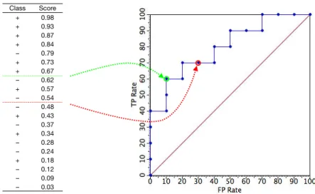
Class Score + 0.98 + 0.93 + 0.87 + 0.84 – 0.79 + 0.73 + 0.67 – 0.62 + 0.57 – 0.54 – 0.48 + 0.43 – 0.37 + 0.34 – 0.28 – 0.24 + 0.18 – 0.12 – 0.09 – 0.03

Figure 1: The table on the left gives the scores assigned by a classifier to 10 pos-itive and 10 negative examples. Each threshold on the classifier’s score results in particular true and false positive rates: e.g., thresholding the score at 0.5 results in 3 misclassified positives (tpr=0.7) and 3 misclassified negatives (fpr=0.3); thresh-olding at 0.65 yieldstpr=0.6 andfpr=0.1. Considering all possible thresholds gives the ROC curve on the right; this curve can also be constructed without ex-plicit reference to scores, by going down the examples sorted on decreasing score and making a step up (to the right) if the example is positive (negative).

tpr+fpr=1. However, we may wish to choose different operating points, for in-stance because false negatives and false positives have different costs. In that case, we need to estimate the noise distribution.

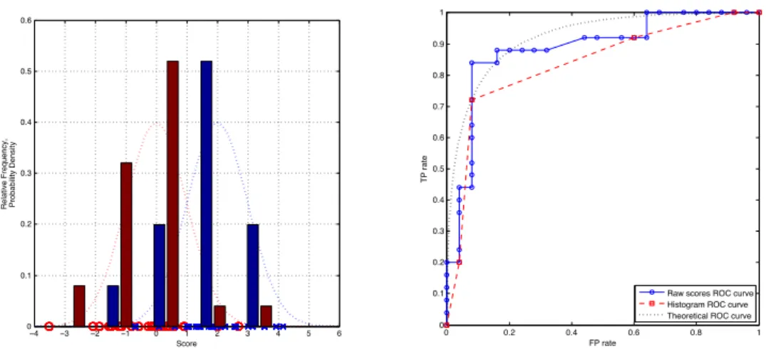
A slight reformulation of the signal detection scenario clarifies its relevance in a machine learning setting. Instead of superimposing random noise on a determinis-tic signal, we can view the resulting noisy signal as coming from a mixture distribution consisting of two component distributions with different means. The detection problem is now to decide, given a received value, from which component distri-bution it was drawn. This is essentially what happens in a binary classification scenario, where the scores assigned by a trained classifier follow a mixture distri-bution with one component for each class. The random variations in the data are translated by the classifier into random variations in the scores, and the classifier’s performance depends on how well the per-class score distributions are separated. Fig. 2 illustrates this for both discrete and continuous distributions. In practice, em-pirical ROC curves and distributions obtained from a test set are discrete because of the finite resolution supplied by the test set. This resolution is further reduced if the classifier only assigns a limited number of different scores, as is the case with decision trees; the histogram example illustrates this.

−4 −3 −2 −1 0 1 2 3 4 5 6 0 0.1 0.2 0.3 0.4 0.5 0.6 Score

Relative Frequency, Probability Density

0 0.2 0.4 0.6 0.8 1 0 0.1 0.2 0.3 0.4 0.5 0.6 0.7 0.8 0.9 1 FP rate TP rate

Raw scores ROC curve Histogram ROC curve Theoretical ROC curve

Figure 2: (left) Artificial classifier ‘scores’ for two classes were obtained by sam-pling 25 points each from two Gaussian distributions with mean 0 and 2, and unit variance. The figure shows the raw scores on thex-axis and normalised histograms obtained by uniform five-bin discretisation. (right) The jagged ROC curve was obtained by thresholding the raw scores as before. The histogram gives rise to a smoothed ROC curve with only five segments. The dotted line is the theoretical curve obtained from the true Gaussian distributions.

Solutions

For convenience we will assume henceforth that score distributions are discrete, and that decision thresholds always fall between actual scores (the results easily generalise to continuous distributions using probability density functions). There is a useful duality between thresholds and scores: decision thresholds correspond to operating points connecting two segments in the ROC curve, and actual scores correspond to segments of the ROC curve connecting two operating points. Let

f(s|+) andf(s|−) denote the relative frequency of positive (negative) examples from a test set being assigned scores. (Note thatsitself may be an estimate of the likelihood p(x|+)of observing a positive example with feature vectorx. We will return to this later.)

Properties of ROC curves

The first property of note is that the true (false) positive rate achieved at a certain decision thresholdtis the proportion of the positive (negative) score distribution to the right of the threshold; that is,tpr(t) =∑s>tf(s|+)andfpr(t) =∑s>tf(s|−). In Fig. 2 , setting the threshold at 1 using the discretised scores gives a true positive rate of 0.72 and a false positive rate of 0.08, as can be seen by summing the bars of the histogram to the right of the threshold. Although the ROC curve doesn’t display thresholds or scores, this allows us to reconstruct the range of thresholds yielding a particular operating point from the score distributions.

If we connect two distinct operating points on an ROC curve by a straight line, the slope of that line segment is equal to the ratio of positives to negatives in the corresponding score interval; that is,

slope(t₁,t₂) =tpr(t2)−tpr(t1)

fpr(t2)−fpr(t1)

=∑t1<s<t2f(s|+)

∑t1<s<t2f(s|−)

Choosing the score interval small enough to cover a single segment of the ROC curve corresponding to scores, it follows that the segment has slopef(s|+)/f(s|−). This can be verified in Fig. 2: e.g., the top-right segment of the smoothed curve has slope 0 because the leftmost bin of the histogram contains only negative examples. For continuous distributions the slope of the ROC curve at any operating point is equal to the ratio of probability densities at that score.

It can happen that slope(t1,t2) <slope(t1,t3)<slope(t2,t3) for t1<t2<t3,

which means that the ROC curve has a ‘dent’ or concavity. This is inevitable when using raw classifier scores (unless the positives and negatives are perfectly separated), but can also be observed in the smoothed curve in the example: the rightmost bin of the histogram has a positive-to-negative ratio of 5, while the next bin has a ratio of 13. Consequently, the two leftmost segments of the ROC curve display a slight concavity. What this means is that performance can be improved by combining those two bins, leading to one large segment with slope 9. In other words, ROC curve concavities demonstrate locally sub-optimal behaviour of a clas-sifier. An extreme case of sub-optimal behaviour occurs if the entire curve is con-cave, or at least below the ascending diagonal: in that case, performance can sim-ply be improved by assigning all test instances the same score, resulting in an ROC curve that follows the ascending diagonal. Aconvex ROC curve is one without concavities.

The AUC statistic

The most important statistic associated with ROC curves is theArea Under (ROC) CurveorAUC. Since the curve is located in the unit square, we have 0≤AUC≤1.

AUC=1 is achieved if the classifier scores every positive higher than every neg-ative;AUC=0 is achieved if every negative is scored higher than every positive.

AUC=1/2 is obtained in a range of different scenarios, including: (i) the classifier assigns the same score to all test examples, whether positive or negative, and thus the ROC curve is the ascending diagonal; (ii) the per-class score distributions are similar, which results in an ROC curve close (but not identical) to the ascending di-agonal; and (iii) the classifier gives half of a particular class the highest scores, and the other half the lowest scores. Notice that, although a classifier withAUCclose to 1/2 is often said to perform randomly, there is nothing random in the third classi-fier: rather, its excellent performance on some of the examples is counterbalanced by its very poor performance on some others.1

1_{Sometimes a linear rescaling 2·AUC−1 called theGini coefficientis preferred, which has a} related use in the assessment of income or wealth distributions using Lorenz curves: a Gini

co-AUChas a very useful statistical interpretation: it is the expectation that a (uni-formly) randomly drawn positive receives a higher score than a randomly drawn negative. It is a normalised version of theWilcoxon-Mann-Whitney sum of ranks test, which tests the null hypothesis that two samples of ordinal measurements are drawn from a single distribution. The ‘sum of ranks’ epithet refers to one method to compute this statistic, which is to assign each test example an integer rank ac-cording to decreasing score (the highest scoring example gets rank 1, the next gets rank 2, etc.); sum up the ranks of then−negatives, which we want to be high; and subtract∑n

−

i=1i=n−(n−+1)/2 to achieve 0 if all negatives are ranked first. The

AUCstatistic is then obtained by normalising by the number of pairs of one pos-itive and one negative,n+n−. There are several other ways to calculateAUC: for instance, we can calculate, for each negative, how many positives precede it, which basically is a column-wise calculation and yields an alternative view ofAUCas the expected true positive rate if the operating point is chosen just before a randomly drawn negative.

Identifying optimal points and the ROC convex hull

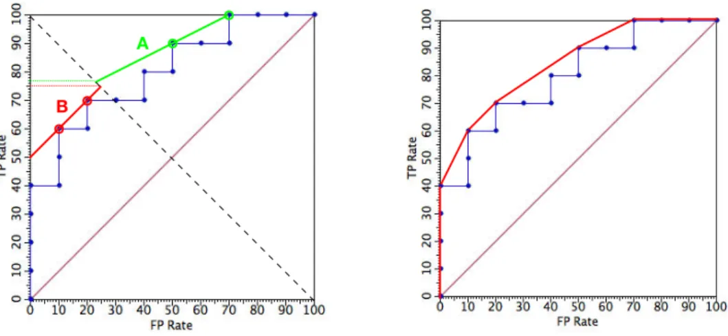
In order to select an operating point on an ROC curve, we first need to specify the objective function we aim to optimise. In the simplest case this will be accuracy, the proportion of correctly predicted examples. Denoting the proportion of posi-tives bypos, we can express accuracy as a weighted average of the true positive and true negative ratespos·tpr+ (1−pos)(1−fpr). It follows that points with the same accuracy lie on a straight line with slopea= (1−pos)/pos; these parallel lines are theisometricsfor accuracy [8]. In order to find the optimal operating point for a given class distribution, we can start with an accuracy isometric through(0,1)and slide it down until it touches the ROC curve in one or more points (Fig. 3 (left)). In the case of a single point this uniquely determines the operating point and thus the threshold. If there are several points in common between the accuracy isometric and the ROC curve, we can make an arbitrary choice, or interpolate stochastically. We can read off the achieved accuracy by intersecting the accuracy isometric with the descending diagonal, on whichtpr=1−fprand therefore the true positive rate at the intersection point is equal to the accuracy associated with the isometric.

We can generalise this approach to any objective function that is a linear com-bination of true and false positive rates. For instance, let predicting class i for an instance of class jincur cost cost(i|j), so for instance the cost of a false pos-itive iscost(+|−) (profits for correct predictions are modelled as negative costs, e.g.cost(+|+)<0). Cost isometrics then have slope

cost(+|−) − cost(−|−)

cost(−|+) − cost(+|+)

efficient close to 0 means that income is approximately evenly distributed. Notice that this Gini coefficient is often called the Gini index, but should not be confused with the impurity measure used in decision tree learning.

4

A

B

1

Figure 3: (left) The slope of accuracy isometrics reflects the class ratio. Isometric A has slope 1/2: this corresponds to having twice as many positives as negatives, meaning that an increase in true positive rate ofxis worth a 2xincrease in false positive rate. This selects two optimal points on the ROC curve. Isometric B corresponds to a uniform class distribution, and selects optimal points which make fewer positive predictions. In either case, the achieved accuracy can be read off on they-axis after intersecting the isometric with the descending diagonal (slightly higher for points selected by A). (right) The convex hull selects those points on an ROC curve which are optimal under some class distribution. The slope of each segment of the convex hull gives the class ratio under which the two end-points of the segment yield equal accuracy. All points under the convex hull are non-optimal. Non-uniform class distributions are simply taken into account by multiplying the class and cost ratio, giving a singleskew ratioexpressing the relative importance of negatives compared to positives.

This procedure of selecting an optimal point on an ROC curve can be gener-alised to select among points lying on more than one curve, or even an arbitrary set of points (e.g., points representing different categorical classifiers). In such scenar-ios, it is likely that certain points are never selected for any skew ratio; such points are said to bedominated. For instance, points on a concave region of an ROC curve are dominated. The non-dominated points are optimal for a given closed interval of skew ratios, and can be joined to form theconvex hullof the given ROC curve or set of ROC points (Fig. 3 (right)).2This notion of the ROC convex hull (sometimes abbreviated to ROCCH) is extremely useful in a range of situations. For instance, if an ROC curve displays concavities, the convex hull represents a discretisation of the scores which achieves higher AUC. Alternatively, the convex hull of a set of categorical classifiers can be interpreted as a hybrid classifier that can reach any point on the convex hull by stochastic interpolation between two neighbouring classifiers [14].

Obtaining calibrated estimates of the class posterior

Recall that each segment of an ROC curve has slopeslope(s) =f(s|+)/f(s|−), wheres is the score associated with the segment, and f(s|+)andf(s|−) are the relative frequencies of positives and negatives assigned scores. Now consider the function

cal(s) = pos·f(s|+)

pos·f(s|+) + (1−pos)·f(s|−) =

slope(s)

slope(s) +a

with a= (1−pos)/pos. Thecalibration map s7→cal(s) adjusts the classifier’s scores to reflect the empirical probabilities observed in the test set. If the ROC curve is convex, slope(s) and cal(s) are monotonically non-increasing with de-creasings, and thus replacing the scoress with cal(s) does not change the ROC curve (other than merging neighbouring segments with different scores but the same slope into a single segment).

Consider decision trees as a concrete example. Once we have trained (and possibly pruned) a tree, we can obtain a score in each leaflby taking the proportion of positive training examples in that leaf: score(l) =p(+|l)/(p(+|l) +p(−|l)). Each leaf of the tree then gives rise to a different segment of the ROC curve, which, by the nature of how the scores were calculated, will be convex. Furthermore, we have that cal(score(l)) =score(l), which means that the tree produces posterior probabilities that are perfectly calibrated with respect to the training set. If we anticipate changes in class distribution we may choose to calibrate with a different

a. For example, if we usea=1, the calibrated scorescal(score(l))are adjusted for a uniform prior.

If the ROC curve is not convex, the mappings7→cal(s)is not monotonic; while the scorescal(s)would lead to improved performance on the data from which the ROC curve was derived, this is very unlikely to generalise to other data, and thus leads to overfitting. This is why, in practice, a less drastic calibration procedure involving the convex hull is applied [6]. Lets1ands2be the scores associated with

the start and end segments of a concavity, i.e.,s1>s2 andslope(s1)<slope(s2).

Letslope(s1s2)denote the slope of the line segment of the convex hull that repairs

this concavity, which impliesslope(s₁)<slope(s₁s₂)<slope(s₂). The calibration map will then map any score in the interval[s1,s2]toslope(s1s2)/(slope(s1s2) +1)

(Fig. 4).

This ROC-based calibration procedure, which is also known as isotonic re-gression[16], not only produces calibrated probability estimates but also improves AUC. This is in contrast with other calibration procedures such as logistic cali-bration which do not bin the scores and therefore don’t change the ROC curve. ROC-based calibration can be shown to achieve lowest Brier score [2], which measures the mean squared error in the probability estimates as compared with the ideal probabilities (1 for a positive and 0 for a negative), among all probabil-ity estimators that don’t reverse pairwise rankings. On the other hand, being a non-parametric method it typically requires more data than parametric methods in

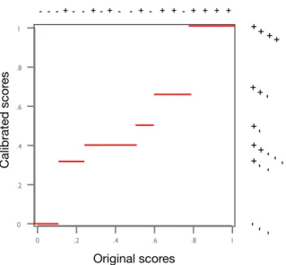
6 + + -+ --+ -+ --+ --- - + + + + + + _{+ +} + + + -+ -+ - - -+ - -- -- -0 .2 .4 .6 .8 1 1 .8 .6 .4 .2 0 Original scores Calibrated scor es

Figure 4: The piece-wise constant calibration map derived from the convex hull in Fig. 3. The original score distributions are indicated at the top of the figure, and the calibrated distributions are on the right. We can clearly see the combined effect of binning the scores and redistributing them over the interval[0,1].

order to estimate the bin boundaries reliably. See Classifier Calibration for further details.

Future Directions

ROC analysis in its original form is restricted to binary classification, and its ex-tension to more than two classes gives rise to many open problems. c-class ROC analysis requiresc(c−1)dimensions, in order to distinguish each possible mis-classification type. Srinivasan proved that basic concepts such as the ROC poly-tope and its linearly interpolated convex hull generalise to thec-class case [15]. In theory, the volume under the ROC polytope can be employed for assessing the quality of a multi-class classifier [7], but this volume is hard to compute as – unlike the two-class case, where the segments of an ROC curve can simply be enumer-ated in O(nlogn) time by sorting the nexamples on their score [5, 9] – there is no simple way to enumerate the ROC polytope. Mossman considers the special case of 3-class ROC analysis, where for each class the two possible misclassifi-cations are treated equally (a so-calledone-versus-rest scenario) [13]. Hand and Till propose the average of all one-versus-rest AUCs as an approximation of the area under the ROC polytope [11]. Various algorithms for minimising a classifier’s misclassification costs by reweighting the classes are considered in [12, 1].

Other research directions include the explicit visualisation of misclassification costs [3], and using ROC analysis to study the behaviour of machine learning

al-gorithms and the relations between machine learning metrics [10].

See also

Accuracy, Classification, Classifier Calibration, Confusion Matrix, Cost-Sensitive Learning and the Class Imbalance Problem, Error Rate, False Negative, False Pos-itive, Gaussian Distribution, Posterior Probability, Precision, Prior Probability, Re-call, Sensitivity, Specificity, True Negative, True Positive.

References and Recommended Reading

[1] Chris Bourke, Kun Deng, Stephen Scott, Robert Schapire, and N. V. Vinod-chandran. On reoptimizing multi-class classifiers. Machine Learning, 71(2-3):219–242, 2008.

[2] Glenn Brier. Verification of forecasts expressed in terms of probabilities.

Monthly Weather Review, 78:1–3, 1950.

[3] Chris Drummond and Robert Holte. Cost curves: An improved method for visualizing classifier performance. Machine Learning, 65(1):95–130, 2006. [4] James Egan. Signal Detection Theory and ROC Analysis. Series in

Cogniti-tion and PercepCogniti-tion. Academic Press, New York, 1975.

[5] Tom Fawcett. An introduction to ROC analysis. Pattern Recognition Letters, 27(8):861–874, 2006.

[6] Tom Fawcett and Alexandru Niculescu-Mizil. PAV and the ROC convex hull.

Machine Learning, 68(1):97–106, 2007.

[7] C´esar Ferri, Jos´e Hern´andez-Orallo, and Miguel Salido. Volume under the ROC surface for multi-class problems. InProceedings of the Fourteenth Eu-ropean Conference on Machine Learning, pages 108–120, 2003.

[8] Peter Flach. The geometry of ROC space: Understanding machine learning metrics through ROC isometrics. In Proceedings of the Twentieth Interna-tional Conference on Machine Learning (ICML 2003), pages 194–201, 2003. [9] Peter Flach. The many faces of ROC analysis in machine learning, July 2004. ICML-04 Tutorial. Notes available fromhttp://www.cs.bris. ac.uk/˜flach/ICML04tutorial/index.html.

[10] Johannes Fuernkranz and Peter Flach. ROC ’n’ Rule learning – towards a better understanding of covering algorithms. Machine Learning, 58(1):39– 77, January 2005.

[11] David Hand and Robert Till. A simple generalization of the area under the ROC curve to multiple class classification problems. Machine Learning, 45(2):171–186, November 2001.

[12] Nicolas Lachiche and Peter Flach. Improving accuracy and cost of two-class and multi-class probabilistic classifiers using ROC curves. In Proceedings of the Twentieth International Conference on Machine Learning (ICML’03), pages 416–423, 2003.

[13] Douglas Mossman. Three-way ROCs. Medical Decision Making, 19:78–89, 1999.

[14] Foster Provost and Tom Fawcett. Robust classification for imprecise environ-ments. Machine Learning, 42(3):203–231, March 2001.

[15] Ashwin Srinivasan. Note on the location of optimal classifiers in n-dimensional ROC space. Technical Report PRG-TR-2-99, Oxford University Computing Laboratory, Oxford, England, 1999.

[16] Barbara Zadrozny and Charles Elkan. Transforming classifier scores into accurate multiclass probability estimates. In Proceedings of the 8th ACM SIGKDD international conference on Knowledge discovery and data mining, pages 694–699. ACM, 2002.

Definitional entries

Area Under Curve

The Area Under Curve (AUC) statistic is an empirical measure of classification performance based on the area under an ROC curve. It evaluates the performance of a scoring classifier on a test set, but ignores the magnitude of the scores and only takes their rank order into account. AUC is expressed on a scale of 0 to 1, where 0 means that all negatives are ranked before all positives, and 1 that all positives are ranked before all negatives.

See: ROC analysis

Decision threshold

The decision threshold of a binary classifier that outputs scores, such as decision trees or naive Bayes, is the value above which scores are interpreted as positive classifi-cations. Decision thresholds can be either fixed if the classifier outputs calibrated scores on a known scale (e.g., 0.5 for a probabilistic classifier), or learned from data if the scores are uncalibrated.

See: ROC analysis

Gini coefficient

The Gini coefficient is an empirical measure of classification performance based on the area under an ROC curve (AUC). Attributed to the Italian statistician Corrado Gini (1884-1965), it can be calculated as 2·AUC−1 and thus takes values in the interval [−1,1], where 1 indicates perfect ranking performance and −1 that all negatives are ranked before all positives.

See: ROC analysis

ROC convex hull

The convex hull of an ROC curve is a geometric construction that selects the points on the curve that are optimal under some class and cost distribution. It is analogous to the Pareto front in multi-objective optimisation.

See: ROC analysis, Classifier calibration

ROC curve

The ROC curve is a plot depicting the trade-off between the true positive rate and the false positive rate for a classifier under varying decision thresholds.