University of Tennessee, Knoxville
Trace: Tennessee Research and Creative
Exchange
Doctoral Dissertations Graduate School
8-2017
Data Analysis Methods using Persistence Diagrams
Andrew Marchese
University of Tennessee, Knoxville, [email protected]
This Dissertation is brought to you for free and open access by the Graduate School at Trace: Tennessee Research and Creative Exchange. It has been accepted for inclusion in Doctoral Dissertations by an authorized administrator of Trace: Tennessee Research and Creative Exchange. For more information, please [email protected].
Recommended Citation
Marchese, Andrew, "Data Analysis Methods using Persistence Diagrams. " PhD diss., University of Tennessee, 2017. https://trace.tennessee.edu/utk_graddiss/4700
To the Graduate Council:
I am submitting herewith a dissertation written by Andrew Marchese entitled "Data Analysis Methods using Persistence Diagrams." I have examined the final electronic copy of this dissertation for form and content and recommend that it be accepted in partial fulfillment of the requirements for the degree of Doctor of Philosophy, with a major in Mathematics.
Vasileios Maroulas, Major Professor We have read this dissertation and recommend its acceptance:
Jan Rosinski, Michael Langston, Haileab Hilafu
Accepted for the Council: Dixie L. Thompson Vice Provost and Dean of the Graduate School (Original signatures are on file with official student records.)
Data Analysis Methods using
Persistence Diagrams
A Dissertation Presented for the
Doctor of Philosophy
Degree
The University of Tennessee, Knoxville
Andrew Marchese
August 2017
c
by Andrew Marchese, 2017 All Rights Reserved.
Acknowledgments
I would like to express my utmost gratitude to my mentor Professor Vasileios Maroulas. Your insight, encouragement, and direction have been invaluable in helping me grow as a researcher and a person. I would also like to express gratitude to each of my committee members. Professor Jan Rosinski has provided valuable insight and feedback during my entire graduate career. Professor Haileab Hilafu has been very supportive and I appreciate our useful conversations and his feedback. Professor Michael Langston helped me to view problems from a different computational and algorithmic point of view and has provided helpful support. Additionally, I want to express gratitude to Dr. Chris Symons for both academic and financial support. Your support and feedback have been instrumental in my success.
Of course, I would not be here without the constant support and motivation of my parents, Terry and Charlie, my brother and sister, Nicholas and Liana, my sister-in-law, Emily, my future mother-in-law, Debbie, my grandmothers, Joan and Angela, and my nephew, Artie. Your encouragement during this endeavor has been unmatched. Moreover, I want to thank my colleagues and friends, including but certainly not limited to Mark Clark, Kai Kang, Brian Allen, Ernest Jum, Eddie Tu, Chase Worley, Gregory Schmidt, Grace McClurkin, Kevin Sonnanburg and many more. A special thank you to Joshua Mike for his collaboration, insight, and friendship over the past few years. I would also like to extend my thanks to both Gary Kulik and Professor Lisa Berger, whose mentorship led me to pursue a career in Mathematics.
Lastly but certainly not least, I would not be where I am today without the seemingly endless support, encouragement, and patience of my fianc´ee Megan Margino. You have been
a constant source of motivation and optimism, and I am deeply grateful to have you in my life.
Abstract
In recent years, persistent homology techniques have been used to study data and dynamical systems. Using these techniques, information about the shape and geometry of the data and systems leads to important information regarding the periodicity, bistability, and chaos of the underlying systems. In this thesis, we study all aspects of the application of persistent homology to data analysis. In particular, we introduce a new distance on the space of persistence diagrams, and show that it is useful in detecting changes in geometry and topology, which is essential for the supervised learning problem. Moreover, we introduce a clustering framework directly on the space of persistence diagrams, leveraging the notion of Fr´echet means. Finally, we engage persistent homology with stochastic filtering techniques. In doing so, we prove that there is a notion of stability between the topologies of the optimal particle filter path and the expected particle filter path, which demonstrates that this approach is well posed. In addition to these theoretical contributions, we provide benchmarks and simulations of the proposed techniques, demonstrating their usefulness to the field of data analysis.
Table of Contents
1 Introduction 1
2 Computational Topology Preliminaries 7
3 Clustering and Classification 17
3.1 Clustering on the space of Persistence Diagrams . . . 18
3.2 Classification on the space of Persistence Diagrams . . . 24
3.3 Discussion and Future Directions . . . 36
4 Data Analysis Results 38 4.1 Computational Preliminaries . . . 38 4.1.1 Hungarian Algorithm . . . 38 4.1.2 k−fold cross-validation . . . 39 4.2 Competing Methods . . . 40 4.3 Clustering Results . . . 42 4.3.1 Synthetic Dataset . . . 43 4.3.2 Real Dataset . . . 44 4.4 Classification Results . . . 45 4.4.1 Synthetic Dataset 1 . . . 45
4.4.2 Synthetic Dataset 2 - A Parameter Sensitivity Test . . . 48
4.4.3 Real Acoustic Signal Dataset . . . 49
5 Topological Stability in State Estimation 57
5.1 Topological Stability . . . 58
5.2 Preliminaries of the Particle Filter. . . 60
5.3 Topological Stability for the Particle Filter . . . 62
5.4 Simulations . . . 65
5.5 Discussion and Conclusion . . . 68
Bibliography 71
List of Tables
4.1 Results for clustering of signals from Eqs. (4.7)-(4.8). . . 44 4.2 Results for clustering of signals from OSU Leaf dataset. . . 44 4.3 Confusion matrix for thedcp classifier on the one channel dataset forp= 5, c =.2. 53 4.4 Confusion matrix for the dc
p classifier on the multichannel dataset for p =
5, c=.2. . . 54 4.5 Differing cardinalities of persistence diagrams corresponding to the differing
List of Figures
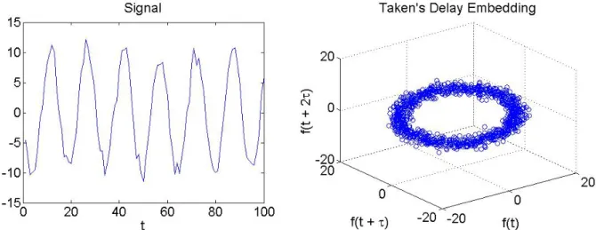
1.1 An example of a persistence diagram Mischaikow and Nanda [61]. . . 3 2.1 Above we depict the signal (left) and its corresponding Taken’s delay
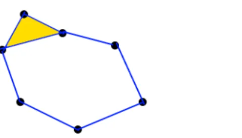
embedding (right) forτ = 10 and d= 3. . . 8 2.2 An example of a 2−dimensional simplicial complex. . . 10 2.3 A cartoon of the simplicial complex K considered for this example.. . . 12 2.4 The construction of ˇCech complexes (right) from the point cloud (left) for
varying epsilon: (a) =.25; (b) =.6; (c) =.8. . . 15 2.5 Above we depict the signal (left), it’s Taken’s delay embedding (center),
and it’s persistent homology (right). Notice the long persistent element corresponding to the cycle in the center of the point cloud. . . 16
3.1 Consider four persistence diagrams, with red points, black points, blue points, and green points. We are interested in the Fr´echet mean of the red persistence diagram and the blue persistence diagram. Notice that both the green persistence diagram and the black persistence diagram minimize Eq.(3.4). . . 20 3.2 A cartoon demonstrating how Algorithm 1 works on a small dataset of
3.3 Consider two persistence diagrams, one with a point at (.1,.2), indicated by the blue square, and one with a point at (.8,.9), indicated by the red circle. Because these points are so far away, the Wasserstein Distance (indicated by the solid black line) finds the optimal bijection as the one mapping both to the diagonal. This results in a distance of .1 between the two diagrams. However, mapping these points to each other (indicated by the dashed line) may be more useful for classification purposes. This mapping of points to each other results in a distance of .7, and this better represents the differences in the persistence diagrams. . . 26 3.4 Left: Noisy small scale features are paired with a single persistent cycle.
Right: As left, but now we see several low persistence points at larger scale, these features alone, which represent the shape of the signal, tell the difference between the two dynamics. . . 27 3.5 Consider two persistence diagrams, one with points represented by red
circles, the other with points represented by blue squares. We compare the Wasserstein distance (on the left) to the proposed dc
p metric (on the right).
Note that the distance between points is computed via the sup norm. Notice how the Wasserstein metric imposes a penalty of .1 to the extra point (the minimal distance to the diagonal), while thedcp imposes a penalty ofc, which will usually be larger. . . 30
4.1 An optimal bijection between two persistence diagrams, one with points in blue, one with points in red. . . 39 4.2 4-fold cross-validation for estimating true error Flock [38]. . . 40 4.3 The methodology through which the signals are processed is visualized above. 41 4.4 An example of a DTW mapping between two signals Zhen et al. [90]. . . 42 4.5 The four classes of signals used for benchmarking the clustering algorithm. . 44 4.6 Examples of signals from the six classes used for benchmarking the clustering
4.7 Sample signals, point clouds, persistence diagrams, and cardinality statistics for (Left) Random walk signals as in Eq. (4.5) and (Right) Bistable signals
as in Eq. (5.4). . . 47
4.8 Synthetic data results forp= 1, ...,5 and c= 0.2,1,5 for Eqs. (4.5) and (5.4). 48 4.9 Sample signals, point clouds, persistence diagrams, and cardinality statistics for (Left) Periodic signals as in Eq. (4.7) and (Right) Doubly Periodic signals as in Eq. (4.8). . . 50
4.10 Results for p= 1, ...,5 and c=.4,1,3,5. . . 51
4.11 Results for competing methods. . . 51
4.12 Results on dataset generated by Eqs. (4.7) and (4.8). . . 51
4.13 Sample signals, point clouds, persistence diagrams, and cardinality statistics for (Left) Class 1 and (Right) Class 2 signals. . . 52
4.14 Single channel results for p= 1, ...,5 andc=.2, .4.. . . 53
4.15 Multichannel results for p= 1, ...,5 and c=.2, .4. . . 53
4.16 Results on acoustic dataset. . . 53
5.1 Cartoon demonstrating how the particles are updated through the particle filter. . . 62
5.2 Ground truth path (top left), particle filter path (top right), ground truth persistence diagram (bottom left), and particle filter path persistence diagram (bottom right) for Equations (1-4) with dynamic noise variance I. . . 66
5.3 Ground truth path (top left), particle filter path (top right), ground truth persistence diagram (bottom left), and particle filter path persistence diagram (bottom right) for Equations (1-4) with dynamic noise variance 0.1I. . . 67
5.4 Ground truth path (top left), particle filter path (top right), ground truth persistence diagram (bottom left), and particle filter path persistence diagram (bottom right) for Equations (5-8). . . 68
Chapter 1
Introduction
In recent years, many signal analysis problems in defense, medicine, computer vision, and signal processing have seen machine learning and data centric approaches to solutions Garrett et al. [40], Sherwin and Sajda [78], Azimi-Sadjadi et al. [7], Dhanalakshmi et al. [28]. Garrett et al. [40] use support vector machines, neural networks, and linear discriminant analysis alongside with features derived from Fourier analysis to classify electroencephalogram and electrocardiogram (EE and EKG) signals. In Sherwin and Sajda [78], the researchers use anomaly detections techniques on EEG signals to detect a difference between musical expects and nonexperts. Azimi-Sadjadi et al. [7] and Dhanalakshmi et al. [28] attempt to classify audio signals using support vector machines and other machine learning techniques.
These types of supervised and unsupervised learning techniques are helpful for specific tasks such as threat detection, disease detection, object recognition, and pattern recognition Srinivas et al. [79], Zhang et al. [89]. Though these classical machine learning approaches produce sufficient results on certain types of data, they rely on extracting features from the data, usually in the form of Fourier coefficients Xu et al. [88], Sahidullah and Saha [72]. While this type of feature extraction is commonplace, this type of method doesn’t take into account theshape andgeometry of the underlying data, properties that can be important to the identification of important signal features such periodicity and chaos Venkataraman et al. [84], Perea and Harer [65]. Due to this, even when an algorithm based on these techniques produces good accuracy, the resulting algorithm can be difficult to interpret.
In order to solve this issue, researchers have taken to utilizing topology to study data in a direction commonly known as topological data analysis Carlsson [21], Carlsson et al. [20]. This type of technique offers a new way to look at data. By treating the underlying dataset as a point cloud and analyzing its topology, researchers are able to draw conclusions about the data set. This type of analysis has seen successful use in the context of supervised machine learning in the fields of medicine, social sciences, and text recognition Nicolau et al. [63], Adcock et al. [2], Lum et al. [53]. For example, in Adcock et al. [2], the researchers extract relevant topological features in conjunction with support vector machines to classify written digits. Due to the intuitive nature of topological data analysis, it is possible to detect properties such as periodicity directly for classification purposes, even when the periodicity may differ widely with respect to period and shape Perea et al. [66].
In terms of signal analysis, the signal is first embedded into a higher dimension using delay embedding theory Takens [81]. The parameters and robustness of this type of delay are well studied. In particular, it has been shown that there are optimal parameters for reconstructing the phase space of the signal for certain types of signals Perea and Harer [65]. Moreover, many studies have empirically shown that the appropriate delay parameter can be estimated by minimizing the autocorrelation of the signal Venkataraman et al. [84], Emrani et al. [35].
Once the signal has been embedded into a k-dimensional point cloud, a topological object is created via one of several different techniques Edelsbrunner and Harer [32]. These techniques, such as ˇCech Complex and Vietoris-Rips Complex, are built through constructing relevant open sets (in our case, open spheres) around each data point, and using properties regarding their intersection to derive a simplicial complex. This simplicial complex has topological properties regarding the amount of connected components, holes, and voids it contains. By varying a scale parameter of the open sets in these constructions, a sequence of simplicial complexes are obtained for a grid of growing scale, leading to information about how long (with respect to scale) objects such as holes and connected components persist. This persistence information is vital for classification and clustering, and contains information regarding the shape of the underlying data Venkataraman et al. [84], Pereira and
de Mello [67], Marchese and Maroulas [55]. This topological information is then summarized in a persistence diagram.
These persistence diagrams, which can be thought of as a collection of points in R2,
capture important topological and geometric information about the underlying signal Perea et al. [66], Venkataraman et al. [84], Emrani et al. [35]. A point (x, y) in the persistence diagram indicates a topological feature born at scale x and persisting until scale y. For example, a 0-dimensional topological feature is a connected component or cluster, a 1-dimensional topological feature is a hole, and so on. The scale y indicates when this hole fills in. The persistence of these topological features is crucial in determining the behavior of the underlying signal and the dynamic generating it. For example, a very persistent 1-dimensional hole corresponds to periodicity in the dynamic, a very persistent 2-dimensional hole may correspond to chaos in the system Emrani et al. [35], Venkataraman et al. [84], Edelsbrunner and Harer [32], Perea and Harer [65]. Small persistence, on the other hand, can indicate difference in the geometry of the underlying system. An example of a persistence diagram can be seen in Fig. 1.1.
Figure 1.1: An example of a persistence diagram Mischaikow and Nanda [61]. Persistence diagrams have recently seen intense active research, including significant successful effort toward facilitating previously challenging computations with them; for example, Wasserstein distance in Kerber et al. [50] or the creation of persistence diagrams with packages such as Dionysus Morozov [62] and Ripser Bauer [10] take advantage of certain
properties of simplicial complexes Chen and Kerber [24]. Moreover, various approaches to define analogues of traditional statistics have been presented. For example, the relationship between persistence diagrams and the noise of the underlying system is studied in Adler et al. [3]. This work demonstrates the lack of noise-induced topological features for large enough feature death value (scale) under Gaussian noise as the number of sample points goes to infinity, indicating the importance of small persistence points in handling noise in the system. The studies Mileyko et al. [59], Turner et al. [83] introduce notions of mean and variance for finite collections of persistence diagrams. The work in Emmett et al. [34] further summarizes the data by extracting kernel density estimates for the distribution of birth and death times, which in turn produces a very rough marginal distribution of a certain homological dimension. This method loses information about individual features in persistence diagrams. A notion of confidence set for persistence diagrams is introduced in Fasy et al. [37], and in Bobrowski et al. [15], kernel densities are introduced for the purposes of data analysis, but the distribution of the underlying persistence diagrams is not explored. Some researchers use these persistence diagrams for classification by first extracting features from them and subsequently using these features in classical machine learning algorithms such as support vector machines and random forests Pereira and de Mello [67], Emrani et al. [35], Zhu [91]. For example, Emrani et al. [35] extracts information regarding the most persistent hole in the data, and uses this alone to classify breathing signals. However, this type of approach necessarily loses information in the persistence diagram and must make assumptions about which type of features are important. To address this issue, it is beneficial to use the entire persistence diagram in the learning process. Venkataraman et al. [84] introduces a 1-Nearest Neighbor classifier using the Wasserstein distance to analyze the classification problem on an action recognition dataset. While this may be viable for classification, the clustering problem in this framework remains unexplored. In Chapter 3, we present a direct solution to this problem by introducing a novel clustering algorithm on the space of persistence diagrams utilizing the notion of Fr´echet means, a generalization of centroids. Moreover, we present results for this clustering scheme and compare to signal feature and signal distance based methods in Chapter4.
While the Wasserstein distance may be ideal in some situations, it is important to note that it loses information about the cardinality of the persistence diagrams and the behavior of small persistence points, that contain relevant information regarding the geometry of the underlying data. We propose a new distance on the space of persistence diagrams taking this into account. This distance is inspired by the study of point processes and characterizes the two important notions of persistence diagram distance - set membership and point location Schuhmacher et al. [75]. Moreover, we explore the notion of means of persistence diagrams under this new distance. Because we cannot simply compute means of persistence diagrams in the traditional sense, we consider a more general Fr´echet mean. We show that this mean is well defined and that it is guaranteed to exist in most real data situations. Theoretical underpinnings for this distance and its corresponding Fr´echet mean are presented in Chapter 3. Moreover, classification benchmark results on real and synthetic datasets are presented in Chapter 4.
Finally, we will draw a connection between these topology based data analysis schemes and stochastic filtering techniques. In some situations, data is observed in a lower dimension than that of the true dynamics, yet we would still like to perform inference on the original space. In order to take this Hidden Markov Mode problem, we must first estimate the true state of the system using the observed state. This is known as the filtering (or smoothing) problem Capp´e et al. [19], Xiong [87], Maroulas and Xiong [58]. We will consider the particle filter, a certain type of filtering algorithm that makes very loose assumptions on the underlying systems dynamics and noise Gordon et al. [42], Ren et al. [70], Doucet et al. [29]. This filtering technique works through drawing many samples, called particles, from the prior probability distribution of the true state, and propagating these particles through the dynamics in order to estimate the posterior distribution of the underlying data, given the available observations. This type of filtering technique has seen applications in many fields such as target tracking and biology Maroulas and Nebenf¨uhr [57]. In particular, we show in Chapter 5 that the topological information contained in the optimal particle filter path and the expected particle filter path are similar. This shows that observing the persistent homology of the mean particle filter path is well posed, in the sense that this persistent homology is close to the persistent homology of the optimal path. Moreover, we provide
simulations demonstrating the connection between persistent homology and particle filtering techniques.
Via the techniques and results explained above, this dissertation provides a holistic analysis of the learning problem on the data space of persistence diagrams. We consider both supervised and unsupervised learning, providing a framework to researchers in many different areas and applications. In particular, our unsupervised learning framework in Chapter 3 is the first of its kind on the space of persistence diagrams, and opens the way for a new way to study signals and dynamical systems. Additionally, through the new distance introduced in Chapter 3, we provide a concrete way to measure small changes in the geometry of dynamical systems that have been hinted at in previous research, but not properly formalized. We show that these small changes in geometry are essential to the classification problem. These theoretical algorithms are implemented and benchmarked in Chapter 4 against real and synthetic datasets. Moreover, we draw a connections between analyzing samples of a dynamical system and analyzing an estimate for the ground truth of the system itself, through the stability result and simulations in Chapter 5.
Chapter 2
Computational Topology
Preliminaries
This chapter will introduce computational topology preliminaries that will be needed for the contributions discussed in later chapters. An interested reader can find a more detailed introduction to the field of computational topology in Edelsbrunner and Harer [32]. In order to perform topological analysis on a signal, it is first necessary to transform the signal into a higher dimension through Takens’ delay embedding Takens [81]. First, we give some topological preliminaries.
Definition 1. Two topological spaces T and H are homeomorphic if there is a continuous bijection f :T →H such that f−1 :H →T is also continuous.
Definition 2. A d−dimensional manifoldM is a topological spaceT such that for for every pointx∈T, there is a neighborhood aroundxhomeomorphic to the opend−ball in Euclidean space.
Definition 3. A map f :M →N between two manifolds is said to be a diffeomorphism if it is differentiable and its inverse f−1 is differentiable. In general, if f is ` times differentiable
it is called a C` diffeomorphism.
Definition 4. A map f : T → H between topological spaces in an embedding if f gives a homeomorphism between T and f(T).
Theorem 2.1 ([81]). Let M be a compact manifold of dimension d and let C2 denote
the space of functions which are twice differentiable and have continuous first and second derivatives. For a C2 diffeomorphism φ : M → M and C2 function f : M →
R, it is a
generic property that Φφ :M →R2m+1 given by
Φφ(x) = (f(x), f(φ(x)), ..., f(φ2m(x))) (2.1)
is an embedding.
Figure 2.1: Above we depict the signal (left) and its corresponding Taken’s delay embedding (right) for τ = 10 and d= 3.
This result guarantees that for a correctly chosen Φ, we can recover the topology of the underlying dynamical system by performing the embedding in Eq. (2.1). We choose Φ to be a delay embedding. In particular, for a time-series f(t), given delay dimension d and delay parameter τ we consider the map
f(t)→(f(t), f(t+τ), ..., f(t+ (d−1)τ)) (2.2)
This type of delay embedding is widely used in the field of topological data analysis Venkataraman et al. [84], Anirudh et al. [5], Zhang et al. [89], Perea et al. [66]. Moreover, the parameters τ and d have been well studied in order to guarantee the underlying topology will be recovered Perea and Harer [65]. An example of this embedding performed on a
signal for d = 3 and τ = 10 can be seen in Figure 2.1. Note that the resulting object is a d−dimensional point cloud P. At a glance, it is obvious that this object has topological and geometric properties, but it is not immediately clear how these can be quantified. For example, examining the topology of the points directly leads to a trivial topology on the space, as they are a set of separate discrete points. However, there is an obvious torus shape that we wish to recover, including a prominent hole in the center. Notice that if we keep track of the points in our delay embedding, we see that this large hole is a result of the periodicity of the signal; this important observation will be expanded upon later. To fully understand this point cloud’s topology, we require persistent homology theory, which will allow us to transform this set of discrete points into a topological summary capturing information about the perceived torus shape and hole in the data.
We now give a brief synopsis of the topological theory required in order to build a family of topological objects from a point cloud of data. Once this family is created, a persistence diagram is created to summarize the information.
Definition 5. A k−dimensional simplex σ is a set of (k+ 1) vertex points,{pi}ki=1+1, and
all convex combinations of these points:
σ= (k+1 X i=1 αipi : k+1 X i=1 αi = 1 and 0≤αi ≤1 ) .
The convex combination of any subset of {pi}ki=1+1 is also a simplex, and is called a face of
σ.
Intuitively, a 0−simplex is a point, a 1−simplex is a line, a 2−simplex is a triangle, et cetera.
Definition 6. An (abstract) simplicial complex is a collection of simplices G such that whenever G contains a simplex σ, G also contains all the faces of σ.
When considering an embedding of an abstract simplicial complex we also require that the intersection of any two simplices is a face of both simplices. For example, two triangles must intersect at a common vertex, a common edge, or not at all. This simplicial complex can be thought of as a higher dimensional generalization of a graph. We observe that this
Figure 2.2: An example of a 2−dimensional simplicial complex.
simplicial complex in Figure 2.2 has certain properties. For example, notice that is has two distinct connected components - one containing all of the points in the “cycle”, and one containing just one point off to the side. Moreover, notice that the “cycle” forms a one dimensional hole. Our goal is to capture this topological information. In order to do this we must understand the relationship between boundaries and edges in a simplicial complex by considering objects called chain groups. We fix a simplicial complex S and an integral domainI.
Definition 7. For a field A and integer j ≥0, a formal sum of j−dimensional simplices is an object of the form P
ajσj, where aj ∈A and σj is a j−simplex.
Definition 8. Thejth chain groupCj(K)is the module of formal sums of thej−dimensional
simplices in S with coefficients in I.
When the simplicial complex K is obvious from context or not needed, we may simply refer to Cj(K) as Cj. By considering a sequence of maps between these chain groups, we obtain information about the structure ofS.
Definition 9. The jth boundary map ∂j :C
j →Cj−1 defined by ∂j(p0, ..., pj) = j X i=0 (−1)i(p0, ..., pi−1, pi+1, ..., pj),
where a j-simplex is mapped to the alternating sum of its j −1−dimensional faces.
We call formal sums of simplicial complexes j−chains for homological dimension j. Moreover, define the boundary of a j−chain to be the formal sum of its j−1-dimensional faces. The following result holds Edelsbrunner and Harer [32].
Lemma 2.1.1. ∂j+1◦∂j = 0 for all integers j ≥0. Thus we have a chain complex C0
∂1 ←− C1
∂2
←− ... ∂`
←− C` such that Im(∂j+1) ⊆ ker(∂j), where ` is the maximum dimension simplex in S, and Im and ker are the image and kernel of the maps.
Definition 10. A subgroup H of a group Gis said to be normal if for all h∈H and g ∈G,
ghg−1 ∈H.
Definition 11. Let H be a subgroup of a group G. The left cosets of H in G is the set
gH ={gh:h∈H}.
Definition 12. For a groupG and a normal subgroup H, define the quotient group G/H to be the set of cosets of H in G.
Given this chain complex and Lemma 2.1.1, it is natural to consider the behavior of the quotient group ker(∂j)/Im(∂j+1).
Definition 13. The jth homology module is defined as the quotient group H
j(S) = ker(∂j)/Im(∂j+1). The jth Betti number βj is the rank of the free part of Hj(K).
We now examine each of these groups in order to understand them in more depth. Fix a homological dimension k and consider ker(∂k). This group contains all chains q in Ck such that∂kq = 0. We call such a chain ak-cycle. Now consider Im(∂k). These are all chains that are k−1-boundaries ofk-chains. We finally come to Hj(S), the group of cycles modded out by boundaries. This group can be thought of as objects that cycles (in the kernel), but are not boundaries (modding out by the kernel). Thus, this corresponds to holes that are not filled in. This contains information regarding structure ofS. In particular, the dimension ofHj(S) overI is the number of j−dimensional holes in S. For example, forj = 0, the dimension of
H0(S), dim(H0(S)) =β0, is the number of connected components in S. For j = 1, it is the
number of 1−dimensional holes. In Figure 2.2, the dimension of H0(S), dim(H0(S)) = β0,
is two (two connected components), the dimension of H1(S), dim(H1(S) = β1, is one (one
1-dimensional hole), and βj is 0 for all j ≥ 1. By constructing these boundary maps for a given simplicial complex, we are able to compute the Betti numbers directly.
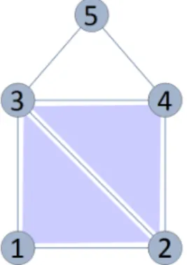
Figure 2.3: A cartoon of the simplicial complex K considered for this example.
Example 1. Consider the simplicial complex depicted in Fig. 2.3. Notice we only have up to 2−simplicies, yielding the chain complex
{0}←−0 C0 ∂1 ←−C1 ∂2 ←−C2 ∂3 ←−C3 ={0}.
We write the simplicial complex as
K ={(1),(2),(3),(4),(5),(1,2),(1,3),(2,3),(2,4),(3,4),(3,5),(4,5),(1,2,3),(2,3,4)}
={v1, v2, v3, v4, v5, e1, e2, e3, e4, e5, e6, e7, f1, f2}
and use this simplex ordering to choose bases for each chain group in order to describe each boundary map as a matrix, as shown below:
∂1 = −1 −1 0 0 0 0 0 1 0 −1 −1 0 0 0 0 1 1 0 −1 −1 0 0 0 0 1 1 0 −1 0 0 0 0 0 1 1 , ∂2 = 1 0 −1 1 1 −1 0 1 0 0 0 0 0 0 .
This organized presentation of the boundary maps enables direct computation of Betti numbers. In this case, ker(∂1) is 3-D, im(∂2) is 2-D, and so H1 is 1-D and β1 = 1. Here,
H1 is generated by the cycle (3,4) + (4,5) + (5,3) =
h
0 0 0 0 1 −1 1 iT
is 1-D and β0 = 1, generated by the lone connected component (1) + (2) + (3) + (4) + (5) =
h
1 1 1 1 1 iT
.
With the computational topology theory established, we are now ready to analyze the point cloud object in Figure 2.1. We need a method for transforming a cloud of points to a family of simplicial complexes. There are several constructions to this end.
Definition 14. For some topological space T, and some covering of T, U = {Uα}α∈A for
some indexing set A, the ˇCech complex C(U) is the simplicial complex whose vertex set is A and a set of points {α0, ..., αk} is a simplex if and only if
Tk
i=0Uαi 6=∅.
For example, in Definition 14, consider T to be a collection of points in Rn and the covering U to be spheres of radius /2 around each point. In this case, we use the notation
C(T) for the ˇCech complex. With this construction, we simply put a k-simplex between
k+ 1 points if their /2 radius spheres have a common nonempty intersection. Figure 2.4 shows an example of a ˇCech complex construction.
Definition 15. Given open setsOi contained inT, the nerveN ofT is an abstract simplicial
complex defined as N ={Oi ⊆T|TOi 6=∅}
Definition 16. A homotopy between continuous functions f : T → H and g :T →H is a continuous map γ :T ×[0,1]→ H such that H(x,0) =f and H(x,1) =g. If this holds, f
and g are said to be homotopic.
Definition 17. Two topological spaces T and H are homotopy equivalent if there are continuous maps f : T → H and g : H → T such that g ◦f and f ◦ g are homotopic to the identity.
This complex forms the nerve of T for a fixed radius . Precisely, the Nerve Theorem conveys the connection between the ˇCech complex and the topology of T Hatcher [44], Edelsbrunner and Harer [31], i.e. that the ˇCech complex andT have the similar topology in some sense (homotopy equivalent). Thus, if we want to understand the spaceT, one needs to study the topology of the corresponding ˇCech complex. However, due to the computational limitations, sometimes we consider an approximation to the ˇCech complex, the Vietoris-Rips complex.
Definition 18. The Vietoris-Rips complex of a finite subset S of a metric space T for some
is the simplicial complex with vertices S such that {p0, ..., pj} is a simplex if and only if
ρ(pi, pv)< for 0≤i, v ≤k, where ρ(·,·) is the metric on T.
In contrast to the ˇCech complex, in the Vietoris-Rips complex a k−simplex is created on points p0, ..., pk−1 when for each pair of vertices the balls around each pair of points
has nonempty intersection. These two constructions are related, in the sense that the ˇCech complex can be approximated with the Vietoris-Rips complex. Consider a ˇCech complex for a fixed radius /2 denotedC and a Vietoris-Rips complex for a fixed radius denoted V R. Then the following approximation holds.
Lemma 2.1.2(Edelsbrunner and Harer [32]). For a fixed radius, we have thatC ⊆V R ⊆
C2
Lemma 2.1.2 says that the Vietoris-Rips complex serves as an approximation to the ˇ
Cech complex, and so we may consider the Vietoris-Rips complex in practice, as it is easier to compute. Observing Definitions 14 and 18 requires a fixed value of . However, it is relevant for the sake of classification to consider what these complexes look like for an increasing sequence of such values. In particular, we are able to track the presence of
n−dimensional voids and connected components as we vary the radius, yielding invaluable information about the topology and geometry of the underlying data. In particular, consider an increasing sequence 1 < ... < j such that we have an associated sequence of nested simplicial complexes, C1 ⊆ ... ⊆ Cj. This sequence of complexes is called a filtration Edelsbrunner and Harer [31]. For each simplicial complexCi, there are associated homology groupsHn(Ci). We consider these homology groups over the fieldZ2 =Z/2Z. In particular, it is possible to keep track of topological features (such as connected components and k -dimensional holes) as the radius changes.
Pertinent topological features such as connected components and holes, corresponding to the Betti numbers for each simplex in the chosen filtration, are kept track of and it is possible to see how long these topological features persist as grows. Of course, eventually when the radius is large enough, all pairs of points will be within and there will be one connected component and no voids. However, what is important is to monitor how
(a)
(b)
(c)
Figure 2.4: The construction of ˇCech complexes (right) from the point cloud (left) for varying epsilon: (a) =.25; (b)=.6; (c) =.8.
these topological features change over increasing . We represent the changing topological features in a chosen complex with a persistence diagram. Consider the complex and fix a homological dimension to consider. For example, settingk = 0 corresponds to keeping track of the connected components of the complex, i.e. β0. Suppose a connected component η is
“born” at time bη, and persists until time dη. The persistence diagram corresponding to a Vietoris-Rips complex consists of birth-death points (bη, dη) for allη that exists for∈G.
Figure 2.5: Above we depict the signal (left), it’s Taken’s delay embedding (center), and it’s persistent homology (right). Notice the long persistent element corresponding to the cycle in the center of the point cloud.
Thus, a persistence diagram is a set of points {(b, d)|b, d ∈ R2 and d > b} where each
point corresponds to a topological feature in a corresponding family of simplicial complexes. In particular, each point (b, d) denoted a topological features being born at radius b and “dying” at radius d. Here, “dying” can be thought of as a homological feature getting filled in with a lower dimensional simplex. The persistence of a feature is defined as d−b, and refers to how “long” (with respect to radius) a topological feature persists before it is filled in. For example, in Figure 2.5, by examining the point cloud in the center image, we expect a hole to form at a relatively small radius and for this hole to persist for a long time. This can be seen in the persistence diagram on the right at the point (.65,7.9). Note that there is a persistence diagram for each homological dimension k, which we combine onto one image.
Chapter 3
Clustering and Classification
The problem of analyzing signals and implementing learning algorithms to perform inference on them is a well studied field with many applications. These range from medical applications involving EEG data Garrett et al. [40], Sherwin and Sajda [78] to acoustic signals with military Azimi-Sadjadi et al. [7] and non-military applications Dhanalakshmi et al. [28].
Recently, topological techniques have been developed to offer a new way to analyze data e.g. see Carlsson [21], Bubenik [16], Bampasidou and Gentimis [9], Xia and Wei [86], Robins and Turner [71]. These techniques have been used in the field of machine learning, with applications in medicine, social sciences, and text recognition Nicolau et al. [63], Adcock et al. [2], Lum et al. [53]. In particular, topological data analysis techniques excel at analyzing point clouds in Rd for some dimension d. Through the use of time-delay embeddings, it is possible to transform the signal classification problem into a point cloud classification problem. Inspired by their original use in reconstructing the phase-space of a dynamical system Takens [81], this delay technique has been effectively used to combine topology and statistics Seversky et al. [76]. Leveraging topological theory, the underlying topological properties of the point cloud produced by this delay embedding are analyzed. Precisely, the persistent homology of the point cloud is represented by a persistence diagram, which can be thought of as a multiset of points in R2, where the (x, y) coordinates signify how long
topological properties of the data persist. In this chapter, we will discuss how this persistence diagram can be used for classification and clustering.
3.1
Clustering on the space of Persistence Diagrams
Clustering is the problem of dividing a dataset into some K number of groups based on some measure of similarity [77]. In this section, we will assume that K is known a priori, but we make no assumptions about the labels of persistence diagrams in the training set. Using the underlying topology of the signal and the dynamic generating the signal can give valuable insight into features vital for class differentiation. Although there has been much work focused on extracting features from persistence diagrams for signal classification or classifying directly on the space of persistence diagrams the same cannot be said for clustering. In Pereira and de Mello [67], the authors transform signals into persistence diagrams and subsequently extract features such as maximum persistence hole (maxi(di−bi)), number of holes, and average lifetime (Pdi−bin ) from persistence diagrams and proceed to use these features to train a traditional clustering algorithm; while this is a first step to using persistence diagrams in the clustering of time-series, these features give a very coarse estimate of the persistence diagrams, and in turn give a summary of the persistence diagram, which is already a topological summary. Though there have been studies focusing on clustering and describing a high-dimensional dataset’s shape and topology using persistent homology Lum et al. [54], Carlsson [21], the problem of time-series clustering directly on the space of persistence diagrams remains unexplored.
For this reason, we instead focus on developing a clustering technique directly on the space of persistence diagrams. In particular, our goal is to introduce a K−means type algorithm on the space of persistence diagrams. In order to achieve this, we need to establish a metric on the space of persistence diagrams, and a notion of “mean” or centers for the persistence diagrams. These concepts are very general and require few assumptions. We start by describing the space of persistence diagrams under a certain metric.
Definition 19. Given two persistence diagrams D1 and D2 and p > 1, define the p
-Wasserstein distance Wp(D1,D2) by Wp(D1,D2) = (inf γ X x∈D1 ||x−γ(x)||∞p)1/p, (3.1)
where γ ranges over all bijections from D1 to D2, p is a fixed parameter, and ||z||∞ =
max(|z1|, ...,|zm|) for z ∈Rm.
Definition 20. Given two persistence diagrams D1 and D2, define the Bottleneck distance
W∞(D1,D2) by
W∞(D1,D2) = inf
γ xsup∈D
1
||x−γ(x)||∞, (3.2)
where γ ranges over all bijections fromD1 to D2, and||z||∞ =max(|z1|, ...,|zm|)forz ∈Rm. In the limit as p goes to infinity, the Wasserstein distance becomes the Bottleneck distance. The Wasserstein distance measures how far off the best possible mapping from
D1 toD2 is over all points. In order to account for cardinality differences in the persistence
diagrams, ad hoc matching to the diagonal is allowed in order to ensure bijectionsγ between
D1 and D2 exist (in other words, any number of features with 0 persistence can be added as
needed).
It is important to note that the space of all finite persistence diagrams under the Wasserstein distance is not complete Mileyko et al. [59]. For example, consider tn to be the topological feature with tn = (bn, dn) = (0,2−n) for n ∈ N, and Dn the persistence diagram containingt1, ..., tn. ThenWp(Dn,Dn+`)< 2n1+`, and so this sequence is cauchy, but the number of points will grow to infinitely as n → ∞, so this sequence does not have a limit in the space. Due to this, when considering the space of persistence diagrams under the Wasserstein distance, we must restrict the space as Pwass ={D|Wp(D,D0)<∞} where
D0 is the persistence diagram only containing the diagonal.
When introducing an algorithm of clustering, it is important to have a notion of center. While it is not obvious how a set of persistence diagrams can be “averaged,” we consider the Fr´echet mean, which is a generalization of a centroid. Consider a probability measureD on the space of (Pwass,B(Pwass)) where B(Pwass) is the Borel σ−algebra on Pwass such that
FWp
Pwass(D1) = Z
Pwass
Wp(D1,D2)2dD(D2)<∞, (3.3)
Definition 21. Given a probability space (Pwass,B(Pwass),D), the Fr´echet variance of D is V arWp D = inf D∈Pwass [FWp Pwass(D) = Z Pwass Wp(D,D2)2dD(D2)], (3.4)
and the Fr´echet expectation or Fr´echet mean of D is
EWp(D) = {D|FPWwassp (D) =V ar
Wp
D }. (3.5)
In [59], it was shown that the space of persistence diagramsPwass admits Fr´echet means under certain types of probability distributions. In particular, this holds for the empirical distribution over a finite set of persistence diagrams; we will be interested in discrete probability distributions for a set {Di}Ti=1 of persistence diagrams. Consider the uniform
distribution T1 PT
i=1δDi over this set. Leveraging this theory, we propose the following
K − means type clustering algorithm. The set of Fr´echet means for a sample diagram
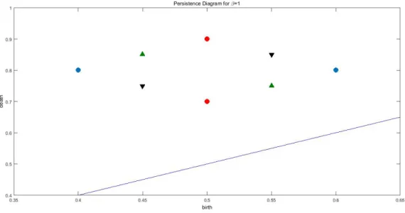
is shown in Fig. 3.1.
Figure 3.1: Consider four persistence diagrams, with red points, black points, blue points, and green points. We are interested in the Fr´echet mean of the red persistence diagram and the blue persistence diagram. Notice that both the green persistence diagram and the black persistence diagram minimize Eq.(3.4).
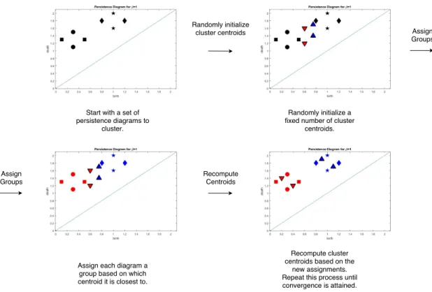
Start with a dataset of persistence diagrams D={Di}Ni=1 to be clustered, with a known
M1(0), ..., MK(0) from D without replacement. These persistence diagrams will act as initial centroids for the algorithm. Then, for each persistence diagram Di ∈ D, assign a label l
(0)
i according to which centroid persistence diagram it is closest too. At this point, for each cluster 1 ≤ J ≤ K, there is a set of persistence diagrams Diags(0)J associated to it. Now, in order to update the centers M1(0), ..., MK(0), define MJ(1) to be the Fr´echet mean of the diagrams in Diags(0)J . This process continues until the labels li(t) =l(it+1) for some iteration
t, for all 1 ≤ i ≤ N. Pseudo-code for this algorithm is presented in Alg. 1, and a single iteration of the algorithm is shown in Fig. 3.2.
Algorithm 1 Clustering on the space of persistence diagrams using Fr´echet means.
1: Input: Persistence Diagrams D={Di}ni=1, number of clusters K, maxiter.
2: Training Phase 3: Initialize Centers
4: for j=1 to K do
5: Randomly initialize centroid diagram Mj(0) for clusterj 6: count = 0
7: while Not Converged do
8: for i=1 ton do Assign Dxi label `
(t) i where ` (t) i = argmin1≤j≤Kd(Dxi, M (t−1) j )
9: for j=1 to K do Compute Mj(t) = Fr´echetMean(DiagsJ(t−1)) where Diags(Jt−1) =
{Dxi|`
(t−1)
i =j}
10: count = count + 1
11: if `(t−1) =`(t) for all 1≤i≤n OR count==maxiter then 12: Converged
13: Return{Mj(T)}K j=1, {`
(T)
i }Ni=1
In order to quantify the effectiveness of the clustering, we consider the associated cost function to Algorithm 1:
G(Diags1, ..., DiagsK) = min M1,...,MK K X i=1 X Dj∈Diagsi (Wp(Dj, Mi))2 (3.6) This cost function is known as the within-cluster sum of squares Shalev-Shwartz and Ben-David [77], Hastie et al. [43]. In particular, it measures the total sum of squared distances from each persistence diagram to its associated cluster centroid diagram. Of course, it is
Figure 3.2: A cartoon demonstrating how Algorithm 1 works on a small dataset of persistence diagrams.
not obvious that the labels will stop changing at some iteration t. The following result guarantees that the algorithm converges to a (local) minimum.
Theorem 3.1. Algorithm 1 converges to a local minimum.
Proof. The algorithm only changes the value of G defined in Eqn. (3.6) at two steps - the update of the Fr´echet MeansM and the update of the cluster assignmentsDiagsJ. We show that in each of these updates, G cannot increase. First fix an iteration t ∈ N and Fr´echet Means M1(t), ..., MK(t). We must show that
K X i=1 X Dj∈Diags(it) Wp(Dj, M (t) i ) 2 ≤ K X i=1 X Dj∈Diags(t −1) i Wp(Dj, M (t) i ) 2 (3.7)
Eqn. (3.7) clearly holds given that the clusters Diags(it) are assigned based on distance to the closest meanM(t). It remains to show the objective function Gof Eqn. (3.6) cannot
the Fr´echet mean of the elements of Diags(it−1). Precisely, Mi(t) is a persistence diagram minimizing X Dj∈Diags (t−1) i Wp(Dj, M (t) i ) 2
Thus, by this definition,
K X i=1 X Dj∈Diags(t −1) i Wp(Dj, M (t) i ) 2 ≤ K X i=1 X Dj∈Diags(t −1) i Wp(x, M (t−1) i ) 2
holds. Since the objective function of the algorithm cannot increase at either of the two update steps, and there are only a finite number of possible labellings, the objective function decreases to a local minimum.
Theorem 3.1 guarantees that the algorithm does not increase the cost of the objective function at every iteration. Because there are only a finite number of permutations of the labels, this guarantees convergence to some labeling which will not change under further runs of the algorithm, which we denote as the local minimum.
For the above clustering scheme, we consider the space of persistence diagrams under the Wasserstein distance. Yet, in order to account for cardinality differences in the persistence diagrams, ad hoc matching to the diagonal is allowed in order to ensure bijections γ
between D1 and D2 exist (in other words, any number of features with 0 persistence
can be added as needed). It is assumed that there are infinitely many points along the diagonal of each persistence diagram with infinite multiplicity Edelsbrunner and Harer [32]. Note that the Wasserstein distance does not explicitly penalize for cardinality differences between persistence diagrams. Differences in cardinality may play an important role in the classification problem. Additionally, allowing mapping to the diagonal can lead to situations where two very different persistence diagrams are considered “close” under the Wasserstein distance. Moreover, through this assumption, the Wasserstein distance necessarily puts a smaller weight on low persistence points. We note some researchers contend that the small persistence points are considered “topological noise” Edelsbrunner et al. [33], Balakrishnan et al. [8], Edelsbrunner and Harer [31], Atienza et al. [6], Pokorny et al. [68]. However, in
line with recent studies, we argue that small persistence points are useful for data analysis Xia and Wei [86], Robins and Turner [71], Bubenik [18]. In the next section, we consider the classification problem, and define a new metric to address these issues.
3.2
Classification on the space of Persistence Diagrams
Whereas in the last section we assumed a dataset of persistence diagrams without any associated labels, in this section we will consider the case of supervised learning. That is, we start with the notion of a dataset of persistence diagrams with a priori knowledge of their associated class labels. Similarly to the clustering framework, several approaches have been taken in order to solve the classification problem using persistence diagrams.One technique researchers have used to is extract a feature vector α ∈ Rd from the persistence diagrams, and use this in conjunction with classical machine learning algorithms (such as neural networks, support vector machines, etc.) Adcock et al. [1], Zhang et al. [89]. Unfortunately, this technique takes a persistence diagram, which is already a topological summary, and further summarizes it into features such as average length of persistence, number of features, etc. This technique necessarily loses information about the underlying topology.
Instead, classification should be done directly on the space of persistence diagrams. Several researchers have tackled the classification problem in this way using the Wasserstein or Bottleneck distance. In Venkataraman et al. [84], the authors implement a nearest neighbor classification algorithm using the Wasserstein distance withp= 1 to classify signals arising from motion sensors on the human body. Similarly, Emrani et. al. Emrani et al. [35] classify acoustic breathing patterns using a distance based technique, allowing for the distinction of wheezing and non-wheezing in patients. The authors of Seversky et al. [76] use both the Wasserstein distance and the p = ∞ Bottleneck distance to classify signals from a wide variety of applications. In addition, the authors propose treating the persistence diagrams as images and training an SVM classifier using these images. Similarly, the researchers in Anirudh et al. [5] treat persistence diagrams as points on a hypersphere using
a probability density function formulation. This representation is then used for classification of signals on a stroke rehabilitation dataset.
Typically, two main distances have been used in the study of persistence diagrams: the Wasserstein distance Kerber et al. [49], Mileyko et al. [59] and the Bottleneck distance Kerber et al. [49]. In terms of theory, the Wasserstein distance is well studied, as shown in the previous section; however, the Wasserstein distance has several drawbacks that make its use questionable in certain applications. Both of these distances require the construction of a bijection between the two persistence diagrams, but this isn’t always possible due to cardinality differences. To get around this, these distances assume infinitely many points with infinite cardinality along the diagonal on each persistence diagram, as discussed in the previous section. This can lead to situations where two very different persistence diagrams are considered close. For example, in Figure 3.3, we compare two persistence diagrams. One has a feature born at time b =.1, while the other has a feature born at b =.8. While their persistence is the same, the scale of the features is extremely different, and in turn these persistence diagrams may be representing two very different point clouds arising from two distinct dynamics. The Wasserstein distance would consider these two topological features to be very similar. Consider the example in Figure3.4. Notice that the persistence diagrams look very similar in terms of large persistence features. However, taking into consideration the differences in small persistence points, these persistence diagrams are very different.
Second, the Wasserstein distance does not explicitly penalize for cardinality differences between persistence diagrams. While this may not inherently seen like a problem, it can be an insurmountable problem in the classification problem. Consider the example in Fig. 4.7, where two very different dynamics may produce persistence diagrams with very different cardinality. This is extremely important when we look at the generating dynamics. The left diagram is generated by a random walk type dynamic, while the right diagram is generated by a multi-stable dynamic. In the context of classification, it is very important to differentiate between these types of dynamics.
In this section, we propose a distance that addresses this issue by directly mapping all points in a persistence diagram. In particular, the proposed distance takes into consideration the geometry of the underlying point cloud by matching small persistence points to each
other. This distance can be thought of as a point matching (similar to the Wasserstein, but we forbid matches to the diagonal), plus a regularization term considering the cardinalities between persistence diagrams. For lower weight on the cardinality difference, the proposed distance will focus more on small persistence points, related to small geometry changes in the underlying data (see Fig. 4.9). On the other hand, for a larger regularization term, the distance will focus on cardinality differences between the persistence diagrams, related to larger changes in the underlying geometry and topology, potentially caused by dynamics and/or noise differences (see Fig. 4.7) Adler et al. [3].
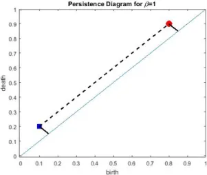
Figure 3.3: Consider two persistence diagrams, one with a point at (.1,.2), indicated by the blue square, and one with a point at (.8,.9), indicated by the red circle. Because these points are so far away, the Wasserstein Distance (indicated by the solid black line) finds the optimal bijection as the one mapping both to the diagonal. This results in a distance of .1 between the two diagrams. However, mapping these points to each other (indicated by the dashed line) may be more useful for classification purposes. This mapping of points to each other results in a distance of .7, and this better represents the differences in the persistence diagrams.
We start by defining the new metric dc
p, to the space of persistence diagrams (Def. 22). Relying on this distance we propose a classification scheme and we show that under mild conditions, the metric space of persistence diagrams is a Polish space and it admits statistical structure, i.e. Fr´echet means and variance.
Definition 22. Consider two persistence diagrams D1 and D2, with cardinalities n and m
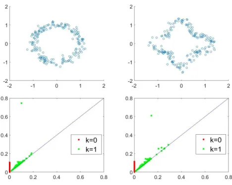
Figure 3.4: Left: Noisy small scale features are paired with a single persistent cycle.
Right: As left, but now we see several low persistence points at larger scale, these features alone, which represent the shape of the signal, tell the difference between the two dynamics.
(y1, ..., ym). Let c >0 and 1< p <∞ be fixed parameters. We define the dcp distance as
dcp(D1,D2) = ( 1 m( minπ∈Πm n X i=1 min(c,||xi−yπ(i)||∞)p+cp|n−m|)) 1 p (3.8)
where Πm is the set of permutations of (1, ..., m). If |D1| > |D2|, define dcp(D1,D2) :=
dc
p(D2,D1).
Proposition 1. The dcp in Eq. (3.8) is a metric on the space of persistence diagrams.
Proof. We adapt the proof from Schuhmacher et al. [75] to the space PW. According to Definition 22, it is clear we have that dcp ≥ 0 and that dcp is symmetric and satisfies the identity. It remains to show the triangle inequality. We consider three persistence diagrams
D1 = (t1, ..., t`),D2 = (u1, ..., un),D3 = (v1, ..., vm). Assume that `≤n and that at most one of the cardinalities is zero. SinceW is a closed and bounded subset ofR2, we consider some
dummy points (ai)i∈N and (bi)i∈N at least distancecfromW and each other. The two cases
We first treat the case when ` ≤n ≤m. Extend the persistence diagram D1 with points
t`+j =aj for 1≤j ≤m−` and similarly forD2 withun+j =bj for 1≤j ≤m−n. This way the cardinality difference is equal to zero in Eq. (3.8). Moreover, after the dummy points have been added in, let η and ν be the minimum permutations fromD1 to D3 and from D3
to D2 respectively. Then, according to Eq. (3.8) and a ≤cpm implying ma ≤ a+c
p(n−m) n , we have dcp(D1,D2) = ( 1 nπmin∈Πn n X i=1 min(c,||ti−uπ(i)||∞)p) 1 p ≤(1 mπmin∈Πm m X i=1 min(c,||ti−uπ(i)||∞)p) 1 p (3.9)
The right hand side of Eq. (3.9) can further be bounded by
(1 m m X i=1 min(c,||ti−vη(i)||∞)p + min(c,||vi−uν(i)||∞)p) 1 p (3.10) ≤(1 m m X i=1 min(c,||ti−vη(i)||∞)p) 1 p + (1 m m X i=1 min(c,||vi−uν(i)||∞)p) 1 p =dcp(D1,D3) +dcp(D3,D2)
Note that in Eq. 3.10, we are mapping from D1 to D3 in the most optimal way (via
permutationη) and then from D3 toD2 in the most optimal way (via permutation ν).
The second case is when `, m≤n. Take η and ν to be the minimum permutations from D1 toD3 and from D3 toD2 respectively as above. Then, similarly, we have that
dcp(D1,D2) = ( 1 nπmin∈Πn n X i=1 min(c,||ti−uπ(i)||∞)p) 1 p ≤(1 m m X i=1 min(c,||ti −vη(i)||∞)p+ min(c,||vi−uν(i)||∞)p) 1 p ≤(1 m m X i=1 min(c,||ti−vη(i)||∞)p) 1 p + (1 m m X i=1 min(c,||vi−uν(i)||∞)p) 1 p =dcp(D1,D3) +dcp(D3,D2)
Intuitively, all points in D1 are matched to points in D2 as best as possible, and then
a regularization term that depends on the remaining difference in cardinality and term cis penalized. Note that for this distance, it is not needed to assume infinitely many points on the diagonal, as in the Wasserstein distance, and thus situations as in Fig. 3.3 are avoided. This distance provides a meaningful distance between two persistence diagrams that also takes into consideration the cardinality difference between them. The parameter c in Eq. (3.8) serves as a penalty on the cardinality difference between persistence diagrams. In particular, a smaller c contributes more weight on the matching between small persistence points, which is important for small geometric differences between signals (see Fig. 4.9). On the other hand, a larger c will largely weight on cardinality differences, which is vital for differentiating between large geometry difference in the point clouds (see Fig. 4.7). These large changes in cardinality can be caused by large differences in dynamic behavior leading to large geometry and topology difference in the point clouds (see Fig. 4.7). In particular, higher scale noise leads to a larger cardinality in persistence diagrams, due to a number of small scale holes appearing Adler et al. [3].
The dc
p distance differs from the Wasserstein distance in the following way. The Wasserstein distance provided in Definition3.2 finds the best possible mapping between two persistence diagrams (where matches to the diagonal are allowed), and then the difference in cardinality is penalized according to the distance to the diagonal. In thedcp metric, points are matched as best as possible from the smaller persistence diagram (in cardinality) to the larger persistence diagram, and then the remaining points are penalized each by c. An example of this can be seen in Fig. 3.5. Note that if two persistence diagrams have the same cardinality and if the optimal bijection from the Wasserstein distance in Eq. (3.2) does not map any points to the diagonal, the Wasserstein distance is equal to the dc
p distance (up to a constant), assumingc is large enough.
We first examine the space of persistence diagrams under this new metric and examine the properties it exhibits. Define the space of persistence diagrams in W ⊂ R2 as P
W,k =
{{x1, ..., xl}|l ≤ k, xi ∈ W,1 ≤ i ≤ l}, where W is a closed and bounded subset of R2 and
k ∈ NS
(a) Wasserstein Distance (b)dc
p Distance
Figure 3.5: Consider two persistence diagrams, one with points represented by red circles, the other with points represented by blue squares. We compare the Wasserstein distance (on the left) to the proposed dc
p metric (on the right). Note that the distance between points is computed via the sup norm. Notice how the Wasserstein metric imposes a penalty of .1 to the extra point (the minimal distance to the diagonal), while the dcp imposes a penalty of c, which will usually be larger.
bounded subset of Rd and as such the associated persistence diagram is bounded in space. Moreover, the number of points in the point clouds considered is bounded depending upon the application (due to sampling rate and observation time). Due to this, it is appropriate to consider the space PW,k for some W and k in real data situations. We show in the next lemma that (PW, dcp) is a complete and separable space.
Lemma 3.1.1. PW under the dcp distance is a complete, separable metric space.
Proof. We first show completeness. Let {Dn}ki=1 be a Cauchy sequence of persistence
diagrams. It is clear that for some k0, we have that j, l ≥ k0 implies |Dj| = |Dl| = k, so we may assume without loss of generality that the associated cardinalities are equal. Fix an >0. Note there isN such that forn, m > N,dc
p(Dn,Dm)< . In particular, since their cardinalities are the same, we have that
dcp(Dn,Dm) = ( 1 kπmin∈Πk k X i=1 ||xn i −xmπ(i)||p∞) 1 p <
and so we have that, for a given point xn i ∈Dn, ||xn i −xmπ(i)||∞<(k) 1 p
where π(i) is the minimal permutation. Thus, there is a sequence of points xni, xnπ+1
n+1(i), x
n+2
πn+2(i), ... such that the distance between
any two points in this sequence is less than 2(k)1p via the triangle inequality, where π
n+α is the minimal permutation between persistence diagrams Dn and Dn+α. This is a Cauchy sequence in W under the inf−norm. Since W is complete, this sequence converges to some limit xi ∈S. Repeating this for each element in Dn, we generate a persistence diagram D∗ consisting of points (x1, ..., xk) chosen as the limits above.
Therefore, for any fixedp, since each sequence above converges to the corresponding limits, there is some N such that for j > N we have ||xji −xi||∞ < This implies that
dcp(Dj,D∗) = ( 1 k πmin∈Πk k X i=1 ||xn i −xπ(i)||p∞) 1 p ≤(1 k k X i=1 ||xn i −xi||p∞) 1 p <(1 kk p)p1 =
Since this sequence converges to a limit in this space, this space is complete. Finally, it remains to show separability. Consider the spacePQT
W of all persistence diagrams with points in QT
W with finitely many points. Then for any persistence diagram D, find
Dq ∈ PQTW such that |D|=|Dq|=k and for all xi ∈D, there is a corresponding yxi ∈Dq such that ||xi−yxi|| p ∞≤. Then dcp(D,Dq) = 1 k( minπ∈Πk k X i=1 ||xi−yπ(i)||p∞)≤ 1 k k X i=1 ||xi−yxi|| p ∞)≤ 1 k k X i=1 =
We now study probability objects on the space of persistence diagrams under the dc p metric through Fr´echet means and variances. We recall these definitions from the previous section in light of our new distance. Fix a closed and bounded subsetW ofR2 and a positive
is the Borelσ−algebra on PW,k such that FPW,k(D1) = Z PW,k dcp(D1,D2)2dD(D2)<∞, (3.11) for all D1 ∈PW,k.
Definition 23. Given a probability space (PW,k,B(PW,k),D), the Fr´echet variance of D is
V arD = inf D∈PW,k [FPW,k(D) = Z PW,k dcp(D,D2)2dD(D2)], (3.12)
and the Fr´echet expectation or Fr´echet mean of D is
E(D) ={D|FPW,k(D) = V arD}. (3.13)
In other words, the Fr´echet mean is any persistence diagram minimizing the Fr´echet variance. Next, we show that the Fr´echet mean exists for a probability distribution over
PW,k.
Lemma 3.1.2. FPW,K(D) is a continuous function.
Proof. Fix some > 0. Consider persistence diagrams D and E such that dc
p(D,E) < min( √ 2 ,maxD1,D2(d c
p(D1,D2)). Then we have that
|FPW,K(D)−FPW,K(E)|=| Z PW,k dcp(D,D1)2dD(D1)− Z PW,k dcp(E,D1)2dD(D1)| =| Z PW,k dcp(D,D1)2−dpc(E,D1)2dD(D1)| ≤ Z PW,k |dc p(D,D1)2 −dcp(E,D1)2|dD(D1) ≤ Z PW,k |(dcp(D,E) +dcp(E,D1))2−dcp(E,D1)2|dD(D1) ≤ Z PW,k |dc p(D,E) 2+dc p(E,D1)2+ 2dcp(D, E)d c p(E,D1)−dcp(E,D1)2|dD(D1) = Z PW,k |dc p(D,E) 2+ 2dc p(D,E)d c p(E,D1)|dD(D1)≤
Theorem 3.2. Let D be a probability measure on (PW,k,B(PW,k)) satisfying Eq. (3.11).
Then E(D)6=∅.
Proof. Let{Di}∞i=1 be a sequence of persistence diagrams such that FPW,k(Di)→V arD. We claim that the space PW,k is totally bounded under the dcp metric. Fix > 0. For each 1≤i≤ k, consider the set of persistence diagrams Di such that Di contains all persistence diagrams with points on agrid of W. LetD=Sk
i=1Di. Then, for any persistence diagram
D∈PW,k, there is D∗ ∈D such that |D|=|D∗| and
dcp(D,D∗) = (1 m( minπ∈Πm m X i=1 min(c,||xi−yπ(i)||∞)p)) 1 p ≤(1 m( m X i=1 p))1p =
Thus, this space is totally bounded and by Lemma 3.1.1, this space is complete. Thus it is compact, and since FPW,K is continuous by Lemma 3.1.2, V arD is attained.
Note that the Fr´echet mean may not be unique, as in Fig. 3.1. The Fr´echet mean can be thought of as a centroid on the data metric space of persistence diagrams. The framework of Theorem 3.2 basically guarantees the mean of a set of persistence diagrams exists in the space PW,k. For a finite set of persistence diagrams Dn = {Di}ni=1, consider the empirical
distribution Dn = n1 Pni=1δDi, that is, the uniform discrete distribution on the finite set of persistence diagrams. Given this distribution, the Fr´echet mean of persistence diagrams Dn is given by E(Dn).
Using this dc
p distance, we consider a classification algorithm for signals via the data space of persistence diagrams. Suppose for each class C1, ..., CL there are corresponding training setsTβl
C1, ..., T
βl
CL containing persistence diagrams corresponding to Betti number βl, for l = 0, ..., BM, where BM is the largest Betti number considered. Then, for a new signal
x(t) with corresponding βl persistence diagram Dβxl, define the average distance to a class
Ck, 1≤k≤L, associated with the Betti number βl by
dβl(x, Ck) = 1 |Tβl Ck| X D∈Tβl Ck dcp(Dβl x ,D) (3.14)
where |Tβl
Ck| is the cardinality of the training set of persistence diagrams corresponding to class k and Betti numberl. We assign the signal x a label ˆC defined as
ˆ C= argmin 1≤k≤L BM X l=0 rldβl(x, Ck) (3.15) where PBM
l=0 rl = 1. The rl’s are weights which determine how much each Betti number βl is considered. Taking all ri’s to be equal gives equal weight to each Betti number. In some situations, prior knowledge may lead to setting some Betti numbers to higher values.
Algorithm 2 Signal classification using persistence diagrams under the dc
p metric.
1: Input 1: New signal x, parametersr1, .., rBM, c, p
2: Input 2: Signals SCk ={x
k i}
|SCk|
i=1 for each class Ck, 1≤k≤L
3: Training Phase
4: for k = 1 to L
![Figure 1.1: An example of a persistence diagram Mischaikow and Nanda [61].](https://thumb-us.123doks.com/thumbv2/123dok_us/529904.2562429/17.918.287.624.610.867/figure-example-persistence-diagram-mischaikow-nanda.webp)