Statistical Topological Data Analysis using Persistence
Landscapes
Peter Bubenik [email protected]
Department of Mathematics Cleveland State University Cleveland, OH 44115-2214, USA
Editor:David Dunson
Abstract
We define a new topological summary for data that we call the persistence landscape. Since this summary lies in a vector space, it is easy to combine with tools from statistics and machine learning, in contrast to the standard topological summaries. Viewed as a random variable with values in a Banach space, this summary obeys a strong law of large numbers and a central limit theorem. We show how a number of standard statistical tests can be used for statistical inference using this summary. We also prove that this summary is stable and that it can be used to provide lower bounds for the bottleneck and Wasserstein distances.
Keywords: topological data analysis, statistical topology, persistent homology, topolog-ical summary, persistence landscape
1. Introduction
Topological data analysis (TDA) consists of a growing set of methods that provide insight to the “shape” of data (see the surveys Ghrist, 2008; Carlsson, 2009). These tools may be of particular use in understanding global features of high dimensional data that are not readily accessible using other techniques. The use of TDA has been limited by the difficulty of combining the main tool of the subject, thebarcode orpersistence diagram with statistics and machine learning. Here we present an alternative approach, using a new summary that we call the persistence landscape. The main technical advantage of this descriptor is that it is a function and so we can use the vector space structure of its underlying function space. In fact, this function space is a separable Banach space and we apply the theory of random variables with values in such spaces. Furthermore, since the persistence landscapes are sequences of piecewise-linear functions, calculations with them are much faster than the corresponding calculations with barcodes or persistence diagrams, removing a second serious obstruction to the wider use of topological methods in data analysis.
In the standard paradigm for TDA, one starts with data that one encodes as a finite set of points in Rn or more generally in some metric space. Then one applies some
ge-ometric construction to which one applies tools from algebraic topology. The end result is a topological summary of the data. The standard topological descriptors are the bar-code and the persistence diagram (Edelsbrunner et al., 2002; Zomorodian and Carlsson, 2005; Cohen-Steiner et al., 2007), which give a multiscale representation of the homology
(Hatcher, 2002) of the geometric construction. Roughly, homology in degree 0 describes the connectedness of the data; homology in degree 1 detects holes or tunnels; homology in degree 2 captures voids; and so on. Of particular interest are the homological features that persist as the resolution changes. We will give precise definitions and an illustrative example of this method, calledpersistent homology or topological persistence, in Section 2. Now let us take a statistical view of this paradigm. We consider the data to be sampled from some underlying abstract probability space. Composing the constructions above, we consider our topological summary to be a random variable with values in some summary spaceS. In detail, the probability space (Ω,F,P) consists of a sample space Ω, aσ-algebra F of events, and a probability measure P. Composing our constructions gives a function X : (Ω,F,P) → (S,A,P∗), where S is the summary space, which we assume has some metric, A is the corresponding Borel σ-algebra, and P∗ is the probability measure on S obtained by pushing forward P along X. We assume that X is measurable and thusX is a random variable with values inS.
Here is a list of what we would like to be able to do with our topological summary. Let X1, . . . , Xnbe a sample of independent random variables with the same distribution as X.
We would like to have a good notion of the mean µof X and the mean Xn of the sample;
know that Xn converges to µ; and be able to calculate Xn(ω), for ω ∈ Ω, efficiently. We
would like to have information the differenceXn−µ, and be able to calculate approximate
confidence intervals related to µ. Given two such samples for random variables X and Y with values in our summary space, we would like to be able to test the hypothesis that µX =µY. In order to answer these questions we also need an efficient algorithm for
calculating distances between elements of our summary space. In this article, we construct a topological summary that we call the persistence landscape which meets these requirements. Our basic idea is to convert the barcode into a function in a somewhat additive manner. The are many possible variations of this construction that may result in more suitable summary statistics for certain applications. Hopefully, the theory presented here will also be helpful in those situations.
We remark that while the persistence landscape has a corresponding barcode and persis-tence diagram, the mean persispersis-tence landscape does not. This is analogous to the situation in which an integer-valued random variable having a Poisson distribution has a summary statistic, the rate parameter, that is not an integer.
We also remark that the reader may restrict our Banach space results results to the perhaps more familiar Hilbert space setting. However we will need this generality to prove stability of the persistence landscape for, say, functions on then-dimensional sphere where n >2.
et al. (2014) use the persistence landscape defined here to study the maltose binding complex and Chazal et al. (2014) apply the bootstrap to the persistence landscape. The persistence landscape is related to the well group defined by Edelsbrunner et al. (2011).
In Section 2 we provide the necessary background and define the persistence landscape and give some of its properties. In Section 3 we introduce the statistical theory of persistence landscapes, which we apply to a few examples in Section 4. In Section 5 we prove that the persistence landscape is stable and that it provides lower bounds for the previously defined bottleneck and Wasserstein distances.
2. Topological Summaries
The two standard topological summaries of data are thebarcodeand thepersistence diagram. We will define a new closely-related summary, thepersistence landscape, and then compare it to these two previous summaries. All of these summaries are derived from thepersistence module, which we now define.
2.1 Persistence Modules
The main algebraic object of study in topological data analysis is the persistence module. A persistence module M consists of a vector space Ma for all a ∈ R and linear maps M(a ≤ b) : Ma → Mb for all a ≤ b such that M(a ≤ a) is the identity map and for all
a≤b≤c,M(b≤c)◦M(a≤b) =M(a≤c).
There are many ways of constructing a persistence module. One example starts with a set of points X = {x1, . . . , xn} in the planeM = R2 as shown in the top left of Figure 1.
To help understand this configuration, we “thicken” each point, by replacing each point, x, with Bx(r) = {y ∈ M | d(x, y) ≤ r}, a disk of fixed radius, r, centered at x. The
resulting union, Xr = Sni=1Br(xi), is shown in Figure 1 for various values of r. For each
r, we can calculate H(Xr), the homology of the resulting union of disks. To be precise,
H(−) denotes Hk(−,F), the singular homology functor in degree k with coefficients in a
field F. So H(Xr) is a vector space that is the quotient of thek-cycles modulo those that
are boundaries. Asr increases, the union of disks grows, and the resulting inclusions induce maps between the corresponding homology groups. More precisely, if r ≤s, the inclusion ιs
r :Xr ,→ Xs induces a map H(ιrs) :H(Xr) →H(Xs). The images of these maps are the persistent homology groups. The collection of vector spaces H(Xr) and linear maps H(ιsr)
is a persistence module. Note that this construction works for any set of points in Rn or
more generally in a metric space.
The union of balls Xr has a nice combinatorial description. The Cech complexˇ , ˇCr(X),
of the set of balls{Bxi(r)} is the simplicial complex whose vertices are the points{xi} and
whosek-simplices correspond tok+ 1 balls with nonempty intersection (see Figure 1). This is also called the nerve. It is a basic result that if the ambient space isRn,Xr is homotopy
equivalent to its ˇCech complex (Borsuk, 1948). So to obtain the singular homology of the union of balls, one can calculate the simplicial homology of the corresponding ˇCech complex. The ˇCech complexes{Cˇr(X)}together with the inclusions ˇCr(X)⊆Cˇs(X) forr≤sform a
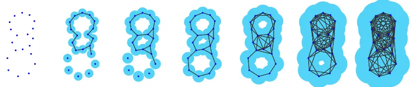
Figure 1: A growing union of balls and the 1-skeleton of the corresponding ˇCech complex. As the radius grows, features—such as connected components and holes—appear and disappear. Here, the complexes illustrate the births and deaths of three holes, homology classes in degree one. The corresponding birth-death pairs are plotted as part of the top left of Figure 2.
The ˇCech complex is often computationally expensive, so many variants have been used in computational topology. A larger, but simpler complex called the Rips complex has as vertices the points xi and has k-simplices corresponding to k+ 1 balls with all pairwise
intersections nonempty. Other possibilities include the witness complexes of de Silva and Carlsson (2004), graph induced complexes by Dey et al. (2013) and complexes built using kernel density estimators and triangulations of the ambient space (Bubenik et al., 2010). Some of these are used in the examples in Section 4.
Given any real-valued function f :S → R on a topological spaceS, we can define the associated persistence module, M(f), whereM(f)(a) = H(f−1((∞, a])) and M(f)(a≤b) is induced by inclusion. Takingf to be the the minimum distance to a finite set of points, X, we obtain the first example.
2.2 Persistence Landscapes
In this section we define a number of functions derived from a persistence module. Examples of each of these are given in Figure 2.
Let M be a persistence module. For a ≤ b, the corresponding Betti number of M, is given by the dimension of the image of the corresponding linear map. That is,
βa,b= dim(im(M(a≤b))). (1)
Lemma 1 If a≤b≤c≤dthenβb,c≥βa,d.
Proof Since M(a≤d) =M(c≤d)◦M(b≤c)◦M(a≤b), this follows from (1).
Our simplest function, which we call the rank function is the functionλ:R2 →Rgiven
by
λ(b, d) = (
βb,d ifb≤d
Now let us change coordinates so that the resulting function is supported on the upper half plane. Let
m= b+d
2 , and h= d−b
2 . (2)
The rescaled rank function is the function λ:R2 →Rgiven by
λ(m, h) = (
βm−h,m+h ifh≥0
0 otherwise.
Much of our theory will apply to these simple functions. However, the following version, which we will call thepersistence landscape, will have some advantages.
First let us observe that for a fixed t∈R,βt−•,t+• is a decreasing function. That is,
Lemma 2 For 0≤h1 ≤h2,
βt−h1,t+h1 ≥βt−h2,t+h2.
Proof Since t−h2 ≤t−h1≤t+h1 ≤t+h2, by Lemma 1, βt−h2,t+h2 ≤βt−h1,t+h1.
Definition 3 The persistence landscape is a function λ : N×R → R, where R denotes
the extended real numbers, [−∞,∞]. Alternatively, it may be thought of as a sequence of functions λk:R→R, where λk(t) =λ(k, t). Define
λk(t) = sup(m≥0 | βt−m,t+m≥k).
The persistence landscape has the following properties.
Lemma 4 1. λk(t)≥0,
2. λk(t)≥λk+1(t), and
3. λk is 1-Lipschitz.
The first two properties follow directly from the definition. We prove the third in the appendix.
To help visualize the graph ofλ:N×R→R, we can extend it to a functionλ:R2→R
by setting
λ(x, t) = (
λ(dxe, t), ifx >0,
0, ifx≤0. (3)
2 4 6 8 10 12 2
4 6 8 10 12
0
birth
death
1 1
2
23 0
0
2 4 6 8 10 12
2
0
λ1
λ2 λ3
2 4 6 8 10 12
2
0
1 1
2 23
0
2 4 6 8 10 12 14 16 2
4 6 8 10
0 2 4 6 8 10 12 14 16
2 4 6 8 10
0
λ1
λ2
2 4 6 8 10 12 14 16
2 4 6 8 10
0
λ1
λ2
2 4 6 8 10 12 14 16
2 4 6 8 10
0
λ1
λ2
Figure 3: Means of persistence diagrams and persistence landscapes. Top left: the rescaled persistence diagrams{(6,6),(10,6)}and{(8,4),(8,8)}have two (Fr´echet) means: {(7,5),(9,7)} and {(7,7),(9,5)}. In contrast their corresponding persistence landscapes (top right and bottom left) have a unique mean (bottom right).
2.3 Barcodes and Persistence Diagrams
All of the information in a (tame) persistence module is completely contained in a multiset of intervals called abarcode(Zomorodian and Carlsson, 2005; Crawley-Boevey, 2012; Chazal et al., 2012). Mapping each interval to its endpoints we obtain the persistence diagram.
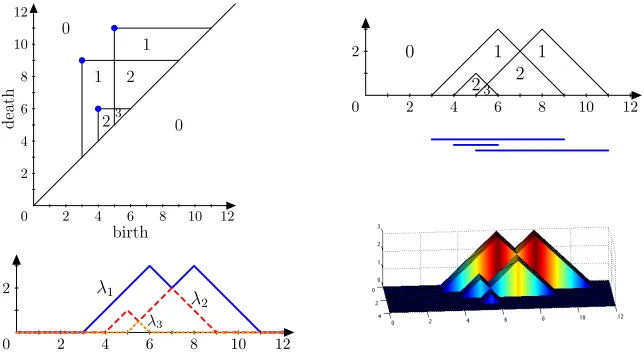
There exist maps in both directions between these topological summaries and our func-tions. For an example of corresponding persistence diagrams, barcodes and persistence landscapes, see Figure 2. Informally, the persistence diagram consists of the “upper-left corners” in our rank function. In the other direction, λ(b, d) counts the number of points in the persistence diagram in the upper left quadrant of (b, d). Informally, the barcode con-sists of the “bases of the triangles” in the rescaled rank function, and the other direction is obtained by “stacking isosceles triangles” whose bases are the intervals in the barcode. We invite the reader to make the mappings precise. For example, given a persistence diagram {(bi, di)}ni=1,
λk(t) =kth largest value of min(t−bi, di−t)+,
wherec+ denotes max(c,0). The fact that barcodes are a complete invariant of persistence modules is central to these equivalences.
The geometry of the space of persistence diagrams makes it hard to work with. For example, sets of persistence diagrams need not have a unique (Fr´echet) mean (Mileyko et al., 2011). In contrast, the space of persistence landscapes is very nice. So a set of persistence landscapes has a unique mean (4). See Figure 3.
function and rescaled rank function, but not in the persistence landscape. However when we pass to the correspondingLp space in Section 2.4, this information disappears.
2.4 Norms for Persistence Landscapes
Recall that for a measure space (S,A, µ), and a function f : S → R defined µ-almost
everywhere, for 1 ≤ p < ∞, kfkp = R
|f|pdµ1
p, and kfk
∞ = ess supf = inf{a | µ{s ∈ S | f(s) > a} = 0}. For 1 ≤ p ≤ ∞, Lp(S) = {f : S →
R | kfkp < ∞} and define
Lp(S) =Lp(S)/∼, wheref ∼gifkf−gk p = 0.
On Rand R2 we will use the Lebesgue measure. On N×R, we use the product of the
counting measure onNand the Lebesgue measure onR. For 1≤p <∞andλ:N×R→R,
kλkpp = ∞ X
k=1 kλkkpp,
where λk(t) = λ(k, t). By Lemma 4(2),kλk∞ =kλ1k∞. If we extend f toλ:R2 →R, as
in (3), we have kλkp=kλkp, for 1≤p≤ ∞.
Ifλis any of our functions corresponding to a barcode that is a finite collection of finite intervals, thenλ∈ Lp(S) for 1≤p≤ ∞, whereS equals
N×RorR2.
Letλbdand λmhdenote the rank function and the rescaled rank function corresponding
to a persistence landscape λ, and let D be the corresponding persistence diagram. Let pers2(D) denote the sum of the squares of the lengths of the intervals in the corresponding barcode, and let pers∞(D) be the length of the longest interval.
Proposition 5 1. kλk1 =kλmhk1 = 21kλbdk1= 14pers2(D), and
2. kλk∞=kλ1k∞= 12pers∞(D). Proof
1. To see thatkλk1 =kλmhkwe remark that both are the volume of the same solid. The
change of coordinates implies that kλmhk1 = 12kλbdk1. If D = {(bi, di)}, then each
point (bi, di) contributes h2i to the volume kλmhk1, where hi = di−2bi. So kλmhk1 = P
ih2i. Finally, pers2(D) = P
i(2hi)2 = 4
P
ih2i.
2. Lemma 4(2) implies that kλk∞=kλ1k∞. If D={(bi, di)}, thenkλk∞= supidi−2bi.
We remark that the quantities in 1 and 2 also equalW2(D,∅)2andW∞(D,∅) respectively (see Section 5 for the corresponding definitions).
3. Statistics with Landscapes
Now let us take a probabilistic viewpoint. First, we assume that our persistence landscapes lie in Lp(S) for some 1 ≤ p < ∞, where S equals
N×R or R2. In this case, Lp(S) is a
3.1 Landscapes as Banach Space Valued Random Variables
Let X be a random variable on some underlying probability space (Ω,F, P), with corre-sponding persistence landscape Λ, a Borel random variable with values in the separable Banach space Lp(S). That is, for ω∈Ω,X(ω) is the data and Λ(ω) =λ(X(ω)) =:λis the
corresponding topological summary statistic.
Now let X1, . . . , Xn be independent and identically distributed copies of X, and let
Λ1, . . . ,Λn be the corresponding persistence landscapes. Using the vector space structure
of Lp(S), the mean landscape Λn is given by the pointwise mean. That is, Λn(ω) = λn,
where
λn(k, t) = 1 n
n
X
i=1
λi(k, t). (4)
Let us interpret the mean landscape. If B1, . . . , Bn are the barcodes corresponding to the
persistence landscapes λ1, . . . , λn, then fork ∈
N and t ∈R, λn(k, t) is the average value
of the largest radius interval centered at t that is contained in k intervals in the barcodes B1, . . . , Bn.
For those used to working with persistence diagrams, it is tempting to try to find a persistence diagram whose persistence landscape is closest to a given mean landscape. While this is an interesting mathematical question, we would like to suggest that the more important practical issue is using the mean landscape to understand the data.
We would like to be able to say that the mean landscape converges to the expected persistence landscape. To say this precisely we need some notions from probability in Banach spaces.
3.2 Probability in Banach Spaces
Here we present some results from probability in Banach spaces. For a more detailed exposition we refer the reader to Ledoux and Talagrand (2011).
Let B be a real separable Banach space with norm k·k. Let (Ω,F, P) be a probability space, and let V : (Ω,F, P) → B be a Borel random variable with values in B. The composite kVk : Ω −V→ B −k·k−→ R is a real-valued random variable. Let B∗ denote the topological dual space of continuous linear real-valued functions on B. For f ∈ B∗, the composite f(V) : Ω−V→ B−→f Ris a real-valued random variable.
For a real-valued random variable Y : (Ω,F, P) → R, the mean or expected value, is given by E(Y) = R
Y dP = R
ΩY(ω) dP(ω). We call an element E(V) ∈ B the Pettis
integral ofV ifE(f(V)) =f(E(V)) for allf ∈ B∗.
Proposition 6 If EkVk<∞, then V has a Pettis integral andkE(V)k ≤EkVk.
Now let (Vn)n∈N be a sequence of independent copies of V. For each n ≥1, let Sn =
V1+· · ·+Vn. For a sequence (Yn) ofB-valued random variables, we say that (Yn)converges almost surely to a B-valued random variable Y, ifP(limn→∞Yn=Y) = 1.
For a sequence (Yn) of B-valued random variables, we say that (Yn) converges weakly
to a B-valued random variableY, if limn→∞E(ϕ(Yn)) =E(ϕ(Y)) for all bounded
contin-uous functions ϕ : B → R. A random variable G with values in B is said to be Gaus-sian if for each f ∈ B∗, f(G) is a real valued Gaussian random variable with mean zero. The covariance structure of a B-valued random variable, V, is given by the expectations E[(f(V)−E(f(V)))(g(V)−E(g(V)))], where f, g ∈ B∗. A Gaussian random variable is determined by its covariance structure. From Hoffmann-Jørgensen and Pisier (1976) we have the following.
Theorem 8 (Central Limit Theorem) Assume that B has type 2. (For example B = Lp(S), with 2≤p <∞.) IfE(V) = 0 andE(kVk2)<∞ then √1
nSn converges weakly to a Gaussian random variableG(V) with the same covariance structure as V.
3.3 Convergence of Persistence Landscapes
Now we will apply the results of the previous section to persistence landscapes. Theorem 7 directly implies the following.
Theorem 9 (Strong Law of Large Numbers for persistence landscapes) Λn→E(Λ) almost surely if and only if EkΛk<∞.
Theorem 10 (Central Limit Theorem for peristence landscapes) Assume p ≥ 2. If EkΛk < ∞ and E(kΛk2) < ∞ then √n[Λn −E(Λ)] converges weakly to a Gaussian random variable with the same covariance structure as Λ.
Proof Apply Theorem 8 to V =λ(X)−E(λ(X)).
Next we apply a functional to the persistence landscapes to obtain a real-valued random variable that satisfies the usual central limit theorem.
Corollary 11 Assume p ≥ 2, EkΛk < ∞ and E(kΛk2) < ∞. For any f ∈ Lq(S) with
1
p +1q = 1, let
Y = Z
S
fΛ =kfΛk1. (5)
Then √
n[Yn−E(Y)] d
−
→N(0,Var(Y)). (6)
where d denotes convergence in distribution and N(µ, σ2) is the normal distribution with
meanµ and variance σ2.
Proof SinceV = Λ−E(Λ) satisfies the central limit theorem inLp(S), for anyg∈Lp(S)∗, the real random variableg(V) satisfies the central limit theorem inRwith limiting Gaussian
law with mean 0 and variance E(g(V)2). If we take g(h) = R
Sf h, where f ∈ Lq(S), with 1
p +
1
3.4 Confidence Intervals
The results of Section 3.3 allow us to obtain approximate confidence intervals for the ex-pected values of functionals on persistence landscapes.
Assume thatλ(X) satisfies the conditions of Corollary 11 and thatY is a corresponding real random variable as defined in (5). By Corollary 11 and Slutsky’s theorem we may use the normal distribution to obtain the approximate (1−α) confidence interval forE(Y) using
Yn±z∗
Sn
√ n,
where Sn2 = n−11 Pn
i=1(Yi −Yn)2, and z∗ is the upper α2 critical value for the normal
distribution.
3.5 Statistical Inference using Landscapes I
Here we apply the results of Section 3.3 to hypothesis testing using persistence landscapes. LetX1, . . . , Xn be an iid copies of the random variableX and letX10, . . . , Xn00 be an iid
copies of the random variable X0. Assume that the corresponding persistence landscapes Λ, Λ0 lie in Lp(S), where p≥2. Letf ∈Lq(S), where 1
p+
1
q = 1. Let Y and Y
0 be defined
as in (5). Let µ = E(Y) and µ0 = E(Y0). We will test the null hypothesis that µ = µ0. First we recall that the sample meanY = n1Pn
i=1Yi is an unbiased estimator ofµand the
sample variance s2Y = n−11 Pn
i=1(Yi−Y)2 is an unbiased estimator of Var(Y) and similarly
forY0 and s2
Y0. By Corollary 11, Y and Y0 are asymptotically normal.
We use the two-sample z-test. Let
z= Y −Y 0
q
S2Y
n +
S2
Y0
n0
,
where the denominator is the standard error for the difference. From this standard score a p-value may be obtained from the normal distribution.
3.6 Choosing a Functional
To apply the above results, one needs to choose a functional, f ∈Lq(S). This choice will
need to be made with an understanding of the data at hand. Here we present a couple of options.
If each λ= Λ(ω) is supported by{1, . . . , K} ×[−B, B], take
f(k, t) = (
1 ift∈[−B, B] and k≤K
0 otherwise. (7)
Then kfΛk1 =kΛk1.
If the parameter values for which the persistence landscape is nonzero are bounded by ±B, then we have a nice choice of functional for the persistence landscape that is unavailable for the (rescaled) rank function. We can choose a functional that is sensitive of the first K dominant homological features. That is, using f in (7), kf λk1 = PK
Under this weaker assumption we can also take fk(t) = k1rχ[−B,B], where r > 1. Then kfΛk1 =P∞k=1k1rkΛk(t)k1.
The condition thatλis supported byN×[−B, B] can often be enforced by using reduced
homology or by applying extended persistence (Cohen-Steiner et al., 2009; Bubenik and Scott, 2014) or by simply truncating the intervals in the corresponding barcode at some fixed values. We remark that certain experimental data may have bounds on the number of intervals. For example, in the protein data considered using the ideas presented here in Kovacev-Nikolic et al. (2014), the simplicial complexes have a fixed number of vertices.
3.7 Statistical Inference using Landscapes II
The functionals suggested in Section 3.6 in the hypothesis test given in Section 3.5 may not have enough power to discriminate between two groups with different persistence in some examples.
To increase the power, one can apply a vector of functionals and then apply Hotelling’s T2 test. For example, considerY = (R
(Λ1−Λ01), . . . , R
(ΛK−Λ0K)), whereK n1+n2−2. This alternative will not be sufficient if the persistence landscapes are translates of each other, (see Figure 7). An additional approach is to compute the distance between the mean landscapes of the two groups and obtain a p-value using a permutation test. This is done in the Section 4.3. This test has been applied to persistence diagrams and barcodes (Chung et al., 2009; Robinson and Turner, 2013).
4. Examples
The persistent homologies in this section were calculated using javaPlex (Tausz et al., 2011) and Perseus by Nanda (2013). Another publicly available alternative is Dionysus by Morozov (2012). In Section 4.2 we use Matlab code courtesy of Eliran Subag that implements an algorithm from Wood and Chan (1994).
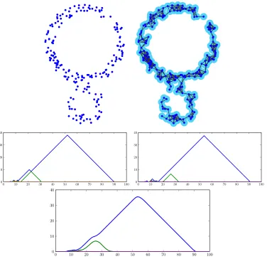
4.1 Linked Annuli
We start with a simple example to illustrate the techniques. Following Munch et al. (2013), we sample 200 points from the uniform distribution on the union of two annuli. We then calculate the corresponding persistence landscape in degree one using the Vietoris-Rips complex. We repeat this 100 times and calculate the mean persistence landscape. See Figure 4.
Note that in the degree one barcode of this example, it is very likely that there will be one large interval, one smaller interval born at around the same time, and all other intervals are smaller and die around the time the larger two intervals are born.
4.2 Gaussian Random Fields
0 10 20 30 40 50 60 70 80 90 100 0
10 20 30 40
0 10 20 30 40 50 60 70 80 90 100
0 10 20 30 40
0 10 20 30 40 50 60 70 80 90 100
0 10 20 30 40
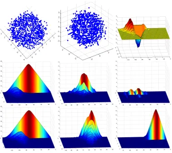
Figure 5: Mean landscapes of Gaussian random fields. The graph of a Gaussian random field on [0,1]2 (top left) and its corresponding mean landscapes (middle row) in degrees 0 and 1. The 0-isosurface of a Gaussian random field on [0,1]3 (top right) and the corresponding mean landscapes in degrees 0, 1 and 2 (bottom row).
has been considered by Adler et al. (2010) and its expected Euler characteristic has been obtained by Bobrowski and Borman (2012).
Here we consider a stationary Gaussian random field on [0,1]2 with autocovariance function γ(x, y) = e−400(x2+y2)
. See Figure 5. We sample this field on a 100 by 100 grid, and calculate the persistence landscape of the sublevel set. For homology in degree 0, we truncate the infinite interval at the maximum value of the field. We calculate the mean persistence landscapes in degrees 0 and 1 from 100 samples (see Figure 5, where we have rescaled the filtration by a factor of 100).
In the Gaussian random field literature, it is more common to consider superlevel sets. However, by symmetry, the expected persistence landscape in this case is the same except for a change in the sign of the filtration.
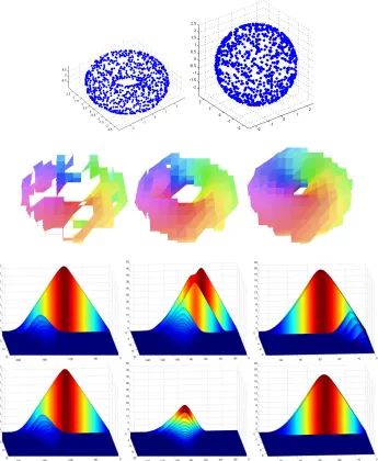
4.3 Torus and Sphere
Here we combine persistence landscapes and statistical inference to discriminate between iid samples of 1000 points from a torus and a sphere inR3with the same surface area, using
the uniform surface area measure as described by Diaconis et al. (2012) (see Figure 6). To be precise, we use the torus given by (r−2)2+z2 = 1 in cylindrical coordinates, and the sphere given by r2 = 2π in spherical coordinates.
For these points, we construct a filtered simplicial complex as follows. First we trian-gulate the underlying space using the Coxeter–Freudenthal–Kuhn triangulation, starting with a cubical grid with sides of length 12. Next we smooth our data using a triangular kernel with bandwidth 0.9. We evaluate this kernel density estimator at the vertices of our simplicial complex. Finally, we filter our simplicial complex as follows. For filtration level −r, we include a simplex in our triangulation if and only if the kernel density estimator has values greater than or equal tor at all of its vertices. Three stages in the filtration for one of the samples are shown in (see Figure 6). We then calculate the persistence landscape of this filtered simplicial complex for 100 samples and plot the mean landscapes (see Figure 6). We observe that the large peaks correspond to the Betti numbers of the torus and sphere. Since the support of the persistence landscapes is bounded, we can use the integral of the landscapes to obtain a real valued random variable that satisfies (6). We use a two-sample z-test to test the null hypothesis that these random variables have equal mean. For the landscapes in dimensions 0 and 2 we cannot reject the null hypothesis. In dimension 1 we do reject the null hypothesis with a p-value of 3×10⁻⁶.
We can also choose a functional that only integrates the persistence landscapeλ(k, t) for certain ranges ofk. In dimension 1, with k= 1 or k = 2 there is a statistically significant difference (p-values of 10−8 and 3×10⁻⁶), but not for k >2. In dimension 2, there is not a significant difference for k = 1, but there is a significant difference for k > 1 (p-value <10−4).
Now we increase the difficulty by adding a fair amount of Gaussian noise to the point samples (see Figure 7) and using only 10 samples for each surface. This time we calculate the L2 distances between the mean landscapes. We use the permutation test with 10,000 repetitions to determine if this distance is statistically significant. There is a significant difference in dimension 0, with a p value of 0.0111. This is surprising, since the mean landscapes look very similar. However, on closer inspection, they are shifted slightly (see Figure 7). Note that we are detecting a geometric difference, not a topological one. This shows that this statistic is quite powerful. There is also a significant difference in dimensions 1 and 2, with p values of 0.0000 and 0.0000, respectively.
5. Landscape Distance and Stability
In this section we define the landscape distance and use it to show that the persistence landscape is a stable summary statistic. We also show that the landscape distance gives lower bounds for the bottleneck and Wasserstein distances. We defer the proofs of the results of this section to the appendix.
p-landscape distance betweenM and M0 by
Λp(M, M0) =kλ−λ0kp.
Similarly, if λand λ0 are the persistence landscapes corresponding to persistence diagrams Dand D0 (Section 2.3), then we define
Λp(D, D0) =kλ−λkp.
Given a real valued function f :X →R on a topological spaceX, letM(f) denote be
the corresponding persistence module defined at the end of Section 2.1.
Theorem 12 (∞-Landscape Stability Theorem) Let f, g:X→R. Then
Λ∞(M(f), M(g))≤ kf−gk∞.
Thus the persistence landscape is stable with respect to the supremum norm. We remark that there are no assumptions on f and g, not even the q-tame condition of Chazal et al. (2012).
LetDbe a persistence diagram. Forx= (b, d)∈D, let`=d−bdenote thepersistence
of x. IfD={xj}, let Persk(D) =
P
j`kj denote the degree-k total persistence of D.
Now let us consider a persistence diagram to be an equivalence class of multisets of pairs (b, d) withb≤d, whereD∼Dq {(t, t)}for anyt∈R. That is, to any persistence diagram,
we can freely adjoin points on the diagonal. This is reasonable, since points on the diagonal have zero persistence. Each persistence diagram has a unique representative ˆDwithout any points on the diagonal. We set |D|=|Dˆ|. We also remark that Persk(D) is well defined.
By allowing ourselves to add as many points on the diagonal as necessary, there exists bijections between any two persistence diagrams. Any bijection ϕ : D −∼=→ D0 can be represented by ϕ : xj 7→ x0j, where j ∈ J with |J| = |D|+|D0|. For a given ϕ, let
xj = (bj, dj),x0j = (b0j, d0j) and εj =kxj−x0jk∞= max(|bj−b0j|,|dj−d0j|).
The bottleneck distance (Cohen-Steiner et al., 2007) between persistence diagrams D and D0 is given by
W∞(D, D0) = inf
ϕ:D ∼
=
−→D0
sup
j
εj,
where the infimum is taken over all bijections from D toD0. It follows that for the empty persistence diagram∅,W∞(D,∅) = 12supj`j.
The ∞-landscape distance is bounded by the bottleneck distance.
Theorem 13 For persistence diagrams D andD0,
Λ∞(D, D0)≤W∞(D, D0).
For p ≥ 1, the p-Wasserstein distance (Cohen-Steiner et al., 2010) between D and D0 is given by
Wp(D, D0) = inf ϕ:D
∼=
−→D0
X
j
εpj
1
p
We remark that the Wasserstein distance gives equal weighting to theεj while the
land-scape distance gives a stronger weighting to εj ifxj has larger persistence. The landscape
distance is most closely related to a weighted version of the Wasserstein distance that we now define. Thepersistence weightedp-Wasserstein distance betweenDand D0 is given by
Wp(D, D0) = inf ϕ:D
∼
=
−→D0
X
j
`jεpj
1
p
.
Note that it is asymmetric.
For the remainder of the section we assume that D and D0 are finite. The following result bounds the p-landscape distance. Recall that `j is the persistence of xj ∈ D and
when ϕ:xj 7→x0j,εj =kxj−x0jk∞
Theorem 14 If n=|D|+|D| then
Λp(D, D0)p ≤ min ϕ:D
∼
=
−→D0
n
X
j=1 `jεpj +
2 p+ 1
n
X
j=1 εpj+1
.
From this we can obtain a lower bound on the p-Wasserstein distance.
Corollary 15 Wp(D, D0)p≥min
1,12hW∞(D,∅) +p+11 i−1Λp(D, D0)p
.
For our final stability theorem, we use ideas from Cohen-Steiner et al. (2010). Let f :X →Rbe a function on a topological space. We say that f istame if for all but finitely
many a ∈ R, the associated persistence module M(f) is constant and finite dimensional on some open interval containing a. For such an f, let D(f) denote the corresponding persistence diagram. If X is a metric space we say that f is Lipschitz if there is some constant c such that |f(x)−f(y)| ≤ c d(x, y) for all x, y ∈ X. We let Lip(f) denote the infimum of all such c. We say that a metric space X implies bounded degree-k total persistence if there is a constant CX,k such that Persk(D(f))≤CX,k for all tame Lipschitz
functions f : X → R such that Lip(f) ≤ 1. For example, as observed by Cohen-Steiner et al. (2010), if X is then-dimensional sphere, thenX=Sn has bounded k-persistence for
k=n+δ for any δ >0, but does not have boundedk-persistence for k < n.
Theorem 16 (p-Landscape stability theorem) Let X be a triangulable, compact met-ric space that implies bounded degree-k total persistence for some real number k ≥1, and let f andg be two tame Lipschitz functions. Then
Λp(D(f), D(g))p≤Ckf−gkp∞−k,
persistence landscape is stable with respect to thep-norm ifp > k, where X has bounded degree-ktotal persistence.
Acknowledgments
The author would like to thank Robert Adler, Frederic Chazal, Herbert Edelsbrunner, Giseon Heo, Sayan Mukherjee and Stephen Rush for helpful discussions. Thanks to Junyong Park for suggesting Hotelling’sT2 test. Also thanks to the anonymous referees who made a number of helpful comments to improve the exposition. In addition, the author gratefully acknowledges the support of the Air Force Office of Scientific Research (AFOSR grant FA9550-13-1-0115).
Appendix A. Proofs
Proof[Proof of Lemma 4(3)] We will prove thatλkis 1-Lipschitz. That is,|λk(t)−λk(s)| ≤
|t−s|, for alls, t∈R.
Lets, t∈R. Without loss of generality, assume thatλk(t)≥λk(s)≥0. Ifλk(t)≤ |t−s|,
thenλk(t)−λk(s)≤λk(t)≤ |t−s|and we are done. So assume that λk(t)>|t−s|.
Let 0 < h < λk(t)− |t−s|. Then t−λk(t) < s−h < s+h < t+λk(t). Thus, by
Lemma 1 and Definition 3, βs−h,s+h ≥ k. It follows that λ
k(s) ≥ λk(t)− |t−s|. Thus
λk(t)−λk(s)≤ |t−s|.
Theorems 12 and 13 follow from the next result which is of independent interest. Follow-ing Chazal et al. (2009), we say that two persistence modules M and M0 are ε-interleaved
if for alla∈Rthere exist linear maps ϕa:Ma→Ma0+ε and ψ:Ma0 →Ma+ε such that for
all a ∈R, ψa+ε◦ϕa =M(a≤ a+ 2ε) and ϕa+ε◦ψa =M0(a≤a+ 2ε) and for all a ≤b
M0(a+ε≤b+ε)◦ϕ
a =ϕb◦M(a≤b) and M(a+ε≤b+ε)◦ψa=ψb◦M0(a≤b). For
persistence modules M and M0 define theinterleaving distance betweenM and M0 by
dI(M, M) = inf(ε|M and M0 are ε-interleaved).
Theorem 17 Λ∞(M, M0)≤dI(M, M0).
Proof Assume that M and M0 are ε-interleaved. Then for t ∈
R and m ≥ ε, the map M(t−m ≤t+m) factors through the mapM0(t−m+ε≤t+m−ε). So by Lemma 1, βt−m+ε,t+m−ε(M0)≥βt−m,t+m(M). Thus by Definition 3,λ0(k, t)≥λ(k, t)−εfor allk≥1. It follows that kλ−λ0k
∞≤ε.
Proof[Proof of Theorem 12] Combining Theorem 17 with the stability theorem of Bubenik and Scott (2014), we have Λ∞(M(f), M(g))≤dI(M(f), M(g))≤ kf−gk∞.
Λ∞(M(D), M(D0))≤dI(M(D), M(D0))≤W∞(D, D0).
Proof [Proof of Theorem 14] Let ϕ : D −→∼= D0 with ϕ(xj) = x0j. Let λ = λ(D) and
λ0=λ(D0). So Λp(D, D0)p =kλ−λ0kpp.
kλ−λ0kp p =
Z
|λ(k, t)−λ0(k, t)|p
=
n
X
k=1 Z
|λk(t)−λ0k(t)|pdt
= Z n
X
k=1
|λk(t)−λ0k(t)|pdt
Fix t. Let uj(t) = λ({xj})(1, t) and vj(t) = λ({x0j})(1, t). For each t, let u(1)(t) ≤ · · · ≤ u(n)(t) denote an ordering of u1(t), . . . , un(t) and define v(k)(t) for 1 ≤ k ≤ n similarly. Then u(k)(t) = λk(t) and v(k)(t) = λ0k(t) (see Figure 2). We obtain the result from the
following where the two inequalities are proven in Lemmata 18 and 19.
kλ−λ0kpp = Z n
X
k=1
|u(k)(t)−v(k)(t)|pdt
≤ Z n
X
k=1
|uk(t)−vk(t)|pdt
=
n
X
j=1 Z
|uj(t)−vj(t)|pdt
≤
n
X
j=1 `jεpj +
2 p+ 1
n
X
j=1 εpj+1.
Lemma 18 Let u1, . . . , un ∈ R and v1, . . . , vn ∈ R. Order them u(1) ≤ · · · ≤ u(n) and v(1)≤ · · · ≤v(n). Then
n
X
j=1
|u(j)−v(j)|p≤
n
X
j=1
|uj−vj|p.
Proof Assume u1 <· · ·< un, v1 <· · ·< vn, and p≥1. Let u and v denote (u1, . . . , un)
and (v1, . . . , vn). Let Σn denote the symmetric group on n letters and letfn : Σn → Rbe
given by fn(σ) = Pnj=1|uj −vσ(j)|p. We will prove by induction that if fn(σ) is minimal
thenσ is the identity, which we denote by 1.
Forn= 1 this is trivial. Forn= 2 assume without loss of generality thatu1 = 0,u2 = 1 and 0 ≤v1 < v2. Let 1 and τ denote the elements of Σ2. Then f(1) =v1p+|1−v2|p and f(τ) =v2p+|1−v1|p. Notice thatf(1)< f(τ) if and only ifvp
1− |1−v1|p < v
p
Now assume that the statement is true for somen≥2. Assume thatfn+1(σ∗) is minimal. Fix 1≤i≤n+ 1. Letu0= (u1, . . . ,uˆi, . . . , un+1) andv0 = (v1, . . . ,vˆσ∗(i), . . . , vn+1), where ˆ·
denotes omission. Sincefn+1(σ∗) is minimal foruandv, it follows thatPnj=1,j6=i|uj−vσ∗(j)|
is minimal for u0 and v0. By the induction hypothesis, for 1≤j < k ≤n+ 1 and j, k6=i, σ∗(j)< σ∗(k). Thereforeσ∗ = 1. Thus, by induction, the statement is true for alln.
HencePn
j=1|u(j)−v(j)|p ≤ Pn
j=1|uj−vj|pifu(1) <· · ·< u(n)andv(1) <· · ·< v(n). The statement in the lemma follows by continuity.
Lemma 19 Let x = (b, d) and x0 = (b0, d0) where b ≤ d and b0 ≤ d0. Let ` = d−b and
ε=kx−x0k
∞. Then kλ({x})−λ({x0})kpp ≤`εp+p+12 εp+1.
Proof Let λ = λ({x}) and λ0 = λ({x0}). First λ
k = λ0k = 0 for k > 1; so kλ−λ0kp =
kλ1−λ01kp. Second λ1(t) = (h− |t−m|)+, where h= d−2b, m= b+2d, andy+ = max(y,0), and similarly for λ01 (see Figure 2).
Fix x and ε. As x0 moves along the square kx−x0k∞=ε,kλ1−λ01k
p
p has a maximum
ifx0 = (a−ε, b+ε). In this casekλ1−λ01kpp= 2
Rh
0 εpdt+ 2 Rε
0 tpdt=`εp+p+12 εp+1. Proof [Proof of Corollary 15] Let ϕ : D −∼=→ D0 be a minimizer for Wp(D, D0), with
cor-responding {εj}. Assume that Wp(D, D0) ≤ 1. Then Wp(D, D0)p = Pnj=1εpj ≤ 1. So for
1≤j≤n,εj ≤1. Combining this with Theorem 14, we have that
Λp(D, D0)p ≤ n
X
j=1
`j+
2 p+ 1
εpj. (8)
Since W∞(D,∅) = max12`j,`j ≤2W∞(D,∅). Hence
Λp(D, D0)p ≤2
W∞(D,∅) + 1 p+ 1
Wp(D, D0)p. (9)
Therefore Wp(D, D0)p ≥ 1 or Wp(D, D0)p ≥ 12
h
W∞(D,∅) + p+11 i−1Λp(D, D0)p. The
statement of the corollary follows.
Theorem 16 follows from the following corollary to Theorem 14 which is of independent interest.
Corollary 20 Let p≥k≥1. Then
Λp(D, D0)p≤W∞(D, D0)p−k
W∞(D,∅)(Persk(D) + Persk(D0))+
1
p+ 1(Persk+1(D) + Persk+1(D 0))
Proof Letϕbe a minimizer for W∞(D, D0) with corresponding{εj}. Ifεj > `2j + `0
j
2 then modify ϕ to pair xj = (bj, dj) with ¯xj = (bj+2dj,bj+2dj) and similarly for x0j. Note that
kxj−x¯jk∞= `2j andkx0j−x¯0jk∞=
`0j
2, soϕis still a minimizer forW∞(D, D0).
Recall that for all j,`j ≤2W∞(D,∅). Sinceϕ is a minimizer for W∞(D, D0), for all j,
εj ≤W∞(D, D0). So applying our choice ofϕto Theorem 14 we have,
Λp(D, D0)p ≤W∞(D, D0)p−k
2W∞(D,∅)
n
X
j=1
εkj + 2 p+ 1
n
X
j=1 εkj+1
.
Now εqj ≤ `j
2 +
`0j
2 q
≤ 12(`j)q+ (`0j)q
for q ≥ 1, where the right hand side follows by the convexity of α(x) =xq forq ≥1. Thus Pn
j=1ε
q
j ≤ 12(Persq(D) + Persq(D0)) forq ≥1.
The result follows.
Proof[Proof of Theorem 16] Theorem 16 follows from Corollary 20 by the following two ob-servations. First, by the stability theorem of Cohen-Steiner et al. (2007),W∞(D(f), D(g))≤ kf −gk∞ and W∞(D(f),∅) ≤ kfk∞. Second, if Persq(D(f)) ≤ CX,q for all tame
Lips-chitz functions f : X → R with Lip(f) ≤ 1, then for general tame Lipschitz functions,
Persq(D(f))≤CX,qLip(f)q.
References
Robert J. Adler and Jonathan E. Taylor. Random Fields and Geometry. Springer Mono-graphs in Mathematics. Springer, New York, 2007. ISBN 978-0-387-48112-8.
Robert J. Adler, Omer Bobrowski, Matthew S. Borman, Eliran Subag, and Shmuel Wein-berger. Persistent homology for random fields and complexes. In Borrowing Strength: Theory Powering Applications—a Festschrift for Lawrence D. Brown, volume 6 ofInst. Math. Stat. Collect., pages 124–143. Inst. Math. Statist., Beachwood, OH, 2010.
Andrew J. Blumberg, Itamar Gal, Michael A. Mandell, and Matthew Pancia. Robust statistics, hypothesis testing, and confidence intervals for persistent homology on metric measure spaces. Found. Comput. Math., 14(4):745–789, 2014. ISSN 1615-3375. doi: 10.1007/s10208-014-9201-4. URLhttp://dx.doi.org/10.1007/s10208-014-9201-4.
Omer Bobrowski and Matthew Strom Borman. Euler integration of Gaussian random fields and persistent homology. J. Topol. Anal., 4(1):49–70, 2012. ISSN 1793-5253.
Karol Borsuk. On the imbedding of systems of compacta in simplicial complexes. Fund. Math., 35:217–234, 1948. ISSN 0016-2736.
Peter Bubenik, Gunnar Carlsson, Peter T. Kim, and Zhi-Ming Luo. Statistical topology via Morse theory persistence and nonparametric estimation. In Algebraic Methods in Statistics and Probability II, volume 516 of Contemp. Math., pages 75–92. Amer. Math. Soc., Providence, RI, 2010.
Gunnar Carlsson. Topology and data. Bull. Amer. Math. Soc. (N.S.), 46(2):255–308, 2009. ISSN 0273-0979.
Gunnar Carlsson, Tigran Ishkhanov, Vin de Silva, and Afra Zomorodian. On the local behavior of spaces of natural images. Int. J. Comput. Vision, 76(1):1–12, 2008. ISSN 0920-5691.
Fr´ed´eric Chazal, David Cohen-Steiner, Marc Glisse, Leonidas J. Guibas, and Steve Y. Oudot. Proximity of persistence modules and their diagrams. In Proceedings of the 25th Annual Symposium on Computational Geometry, SCG ’09, pages 237–246, New York, NY, USA, 2009. ACM. ISBN 978-1-60558-501-7.
Frederic Chazal, Vin de Silva, Marc Glisse, and Steve Oudot. The structure and stability of persistence modules. arXiv:1207.3674 [math.AT], 2012.
Fr´ed´eric Chazal, Marc Glisse, Catherine Labru`ere, and Bertrand Michel. Optimal rates of convergence for persistence diagrams in topological data analysis. 2013. arXiv:1305.6239 [math.ST].
Fr´ed´eric Chazal, Brittany Terese Fasy, Fabrizio Lecci, Alessandro Rinaldo, and Larry Wasserman. Stochastic convergence of persistence landscapes and silhouettes. Symposium on Computational Geometry (SoCG), 2014.
Chao Chen and Michael Kerber. An output-sensitive algorithm for persistent homology.
Comput. Geom., 46(4):435–447, 2013. ISSN 0925-7721.
Moo K. Chung, Peter Bubenik, and Peter T. Kim. Persistence diagrams in cortical surface data. InInformation Processing in Medical Imaging (IPMI) 2009, volume 5636 ofLecture Notes in Computer Science, pages 386–397, 2009.
David Cohen-Steiner, Herbert Edelsbrunner, and John Harer. Stability of persistence dia-grams. Discrete Comput. Geom., 37(1):103–120, 2007. ISSN 0179-5376.
David Cohen-Steiner, Herbert Edelsbrunner, and John Harer. Extending persistence using Poincar´e and Lefschetz duality. Found. Comput. Math., 9(1):79–103, 2009. ISSN 1615-3375.
David Cohen-Steiner, Herbert Edelsbrunner, John Harer, and Yuriy Mileyko. Lipschitz functions haveLp-stable persistence. Found. Comput. Math., 10(2):127–139, 2010. ISSN
1615-3375.
Vin de Silva and Gunnar Carlsson. Topological estimation using witness complexes. Euro-graphics Symposium on Point-Based Graphics, 2004.
Vin De Silva and Robert Ghrist. Coverage in sensor networks via persistent homology.
Algebr. Geom. Topol., 7:339–358, 2007a.
Vin De Silva and Robert Ghrist. Homological sensor networks. Notic. Amer. Math. Soc., 54(1):10–17, 2007b.
Mary-Lee Dequ´eant, Sebastian Ahnert, Herbert Edelsbrunner, Thomas M. A. Fink, Earl F. Glynn, Gaye Hattem, Andrzej Kudlicki, Yuriy Mileyko, Jason Morton, Arcady R. Mushe-gian, Lior Pachter, Maga Rowicka, Anne Shiu, Bernd Sturmfels, and Olivier Pourqui´e. Comparison of pattern detection methods in microarray time series of the segmentation clock. PLoS ONE, 3(8):e2856, 08 2008.
Tamal Krishna Dey, Fengtao Fan, and Yusu Wang. Graph induced complex on point data. In
Proceedings of the Twenty-ninth Annual Symposium on Computational Geometry, SoCG ’13, pages 107–116, New York, NY, USA, 2013. ACM. ISBN 978-1-4503-2031-3.
Persi Diaconis, Susan Holmes, and Mehrdad Shahshahani. Sampling from a manifold. arXiv:1206.6913 [math.ST], 2012.
Herbert Edelsbrunner, David Letscher, and Afra Zomorodian. Topological persistence and simplification. Discrete Comput. Geom., 28(4):511–533, 2002. ISSN 0179-5376. Discrete and computational geometry and graph drawing (Columbia, SC, 2001).
Herbert Edelsbrunner, Dmitriy Morozov, and Amit Patel. Quantifying transversality by measuring the robustness of intersections. Found. Comput. Math., 11(3):345–361, 2011. ISSN 1615-3375.
Brittany Terese Fasy, Fabrizio Lecci, Alessandro Rinaldo, Larry Wasserman, Sivaraman Balakrishnan, and Aarti Singh. Confidence sets for persistence diagrams. Ann. Statist., 42(6):2301–2339, 2014. ISSN 0090-5364. doi: 10.1214/14-AOS1252. URL http://dx. doi.org/10.1214/14-AOS1252.
Robert Ghrist. Barcodes: the persistent topology of data. Bull. Amer. Math. Soc. (N.S.), 45(1):61–75, 2008. ISSN 0273-0979.
Allen Hatcher. Algebraic Topology. Cambridge University Press, Cambridge, 2002. ISBN 0-521-79160-X; 0-521-79540-0.
Giseon Heo, Jennifer Gamble, and Peter T. Kim. Topological analysis of variance and the maxillary complex. J. Amer. Statist. Assoc., 107(498):477–492, 2012. ISSN 0162-1459.
J. Hoffmann-Jørgensen and G. Pisier. The law of large numbers and the central limit theorem in Banach spaces. Ann. Probability, 4(4):587–599, 1976.
Michel Ledoux and Michel Talagrand. Probability in Banach Spaces. Classics in Mathemat-ics. Springer-Verlag, Berlin, 2011. ISBN 978-3-642-20211-7. Isoperimetry and processes, Reprint of the 1991 edition.
Yuriy Mileyko, Sayan Mukherjee, and John Harer. Probability measures on the space of persistence diagrams. Inverse Problems, 27(12):124007, 22, 2011. ISSN 0266-5611.
Nikola Milosavljevi´c, Dmitriy Morozov, and Primoˇz ˇSkraba. Zigzag persistent homology in matrix multiplication time. InComputational Geometry (SCG’11), pages 216–225. ACM, New York, 2011.
Dimitriy Morozov. Dionysus: a C++ library with various algorithms for computing per-sistent homology. Software available at http://www.mrzv.org/software/dionysus/, 2012.
Elizabeth Munch, Paul Bendich, Katharine Turner, Sayan Mukherjee, Jonathan Mat-tingly, and John Harer. Probabilistic fr´echet means and statistics on vineyards. 2013. arXiv:1307.6530 [math.PR].
Vidit Nanda. Perseus: the persistent homology software. Software available at http: //www.math.rutgers.edu/~vidit/perseus/index.html, 2013.
Monica Nicolau, Arnold J. Levine, and Gunnar Carlsson. Topology based data analysis identifies a subgroup of breast cancers with a unique mutational profile and excellent survival. Proc. Nat. Acad. Sci., 108(17):7265–7270, 2011.
Andrew Robinson and Katharine Turner. Hypothesis testing for topological data analysis. 2013. arXiv:1310.7467 [stat.AP].
Andrew Tausz, Mikael Vejdemo-Johansson, and Henry Adams. Javaplex: a research soft-ware package for persistent (co)homology. Softsoft-ware available at http://code.google. com/javaplex, 2011.
Katharine Turner, Yuriy Mileyko, Sayan Mukherjee, and John Harer. Fr´echet means for distributions of persistence diagrams. Discrete Comput. Geom., 52(1):44–70, 2014.
Andrew T. A. Wood and Grace Chan. Simulation of stationary Gaussian processes in [0,1]d. J. Comput. Graph. Statist., 3(4):409–432, 1994. ISSN 1061-8600.

![Figure 5: Mean landscapes of Gaussian random fields. The graph of a Gaussian randomfield on [0, 1]2 (top left) and its corresponding mean landscapes (middle row) indegrees 0 and 1](https://thumb-us.123doks.com/thumbv2/123dok_us/9800475.1966000/14.612.133.481.88.432/figure-landscapes-gaussian-gaussian-randomeld-corresponding-landscapes-indegrees.webp)