Specification Analysis of Option Pricing Models Based on Time- Changed Levy Processes

Specification Analysis of Option Pricing Models

Based on Time-Changed L´evy Processes

JING-ZHI HUANG AND LIUREN WU

Huang is from Smeal College of Business, Penn State University. Wu is from Zicklin School of Business, Baruch College (CUNY). We are grateful to Rick Green (the editor), an anonymous referee, Menachem Brenner, Peter Carr, Robert Engle, Steve Figlewski, Martin Gruber, Jean Helwege, Marti Subrahmanyam, and Rangarajan Sundaram for helpful comments and discussions. We thank seminar participants at Baruch College, the University of Notre Dame, Salomon Smith Barney, and Washington University in St. Louis for helpful comments. We also thank Sandra Sizer Moore for her editing.

ABSTRACT

We analyze the specifications of option pricing models based on time-changed L´evy processes. We classify option pricing models based on the structure of the jump component in the underlying return process, the source of stochastic volatility, and the specification of the volatility process itself. Our estimation of a variety of model specifications indicates that to better capture the behavior of the S&P 500 index options, we need to incorporate a high frequency jump component in the return process and generate stochastic volatilities from two different sources, the jump component and the diffusion component.

Although researchers have proposed and tested various extensions of the Black and Scholes (1973) model, they have yet to find a model that can capture both the time series and cross-sectional properties of equity index options. The significance of this task is enormous. First, to price and hedge options, we need to explain the behavior of option prices across strike prices and maturities. Second, the in-formation from the options market helps us understand the underlying asset return dynamics as the option price behavior reveals important information about the conditional risk-neutral distributions of the underlying return over different horizons.

In this paper, we present a unified framework that synthesizes the ongoing efforts to identify the “true” dynamics of the underlying return process by performing a specification analysis of option pric-ing models. We then apply this analysis to S&P 500 index options and empirically investigate some open issues regarding the equity index return dynamics.

The specification analysis we develop here is based on the theoretical framework of time-changed L´evy processes proposed by Carr and Wu (2003b). A L´evy process is a continuous time stochastic process with independent stationary increments. In addition to the Brownian motion and the compound Poisson jump process used in the traditional option pricing literature, the class of L´evy processes also includes other jump processes that exhibit higher jump frequencies and thus may better capture the dynamics of equity indexes. On the other hand, a time change is a monotonic transformation of the time variable. Stochastic volatility can be generated by applying random time changes to the individual components of a L´evy process. For example, we can apply different time changes separately to the diffusion component and the jump component of a L´evy process so that stochastic volatility can be generated from both components. Therefore, the framework of time-changed L´evy processes can be used to generate a wide class of jump-diffusion stochastic volatility models.

Within the class of time-changed L´evy processes, we classify model specifications into three sep-arate but interrelated dimensions: the choice of a jump component in the asset return process, the identification of the sources for stochastic volatility, and the specification of the volatility process it-self. Such a classification scheme encompasses almost all option pricing models in the literature and provides a framework for future modeling efforts.

Based on this framework, we design and estimate a series of models using S&P 500 index options data and test the relative goodness-of-fit of each specification. Our specification analysis focuses on addressing two important questions on model design. (Q1) What type of jump structure best describes the underlying price movement and the return innovation distribution? (Q2) Which component, the jump component or the diffusion component, determines the time variation of return volatility?

The empirical analysis in this paper focuses on the performance of 12 option pricing models that are generated by a combination of three jump processes and four stochastic volatility specifications. The three jump processes include the standard compound Poisson jump process (MJ) used in Merton (1976), the variance-gamma jump model (VG) of Madan, Carr, and Chang (1998), and the log stable model (LS) of Carr and Wu (2003a). The compound Poisson jump model (MJ) generates a finite number of jumps within any finite time interval. In contrast, both VG and LS allow an infinite number of jumps within any finite interval and hence are better suited to capture highly frequent discontinuous movements in the underlying asset return. We choose these three jump processes to address the question raised in (Q1).

The stochastic volatility specifications include the traditional specification in Bates (1996) and Bakshi, Cao, and Chen (1997), in which the instantaneous variance of the diffusion component is stochastic but the arrival rate of the jump component is constant. We also introduce new specifications that allow us to generate stochastic volatility separately from the jump and diffusion components. These new stochastic volatility specifications are designed to address the question raised in (Q2).

Our estimation results show that in capturing the behavior of the S&P 500 index options, models based on VG and LS outperform those based on the compound Poisson process (MJ). This performance ranking is robust to variations in the stochastic volatility specification and holds for both in-sample and out-of-sample tests. Our results suggest that the market prices index options as if there are many discontinuous price movements of different magnitudes in the S&P 500 index. This implication favors incorporating high frequency jumps such as VG and LS in the underlying asset return process.

The estimation results also show that variations in the index return volatility come from two separate sources: the instantaneous variance of the diffusion component and the arrival rate of the jump com-ponent. One implication of this finding is that the intensities of both small and large index movements

vary over times and they vary separately. Furthermore, the model parameter estimates indicate that the return volatility generated from the diffusion and the jump components show different risk-neutral dy-namics. The diffusion-induced volatility exhibits larger instantaneous variation, but the jump-induced return volatility shows much higher persistence. As a result, the behavior of short-term options is in-fluenced more by the randomness from the diffusive movements, but the behavior of long-term options is mostly influenced by the randomness in the arrival rate of jumps.

The empirical results from our specification analysis provide further support for option pricing models that include both jumps and stochastic volatility. Nevertheless, our results also illustrate the importance of choosing the right jump structure and designing a good stochastic volatility specifica-tion. We find that the option pricing model performance can be significantly improved by including high-frequency jumps in the underlying return process and by generating stochastic return volatility separately from the jump and diffusion components.

The paper is organized as follows. Section I discusses the studies that form the background for our paper. Section II constructs option pricing models through time changing L´evy processes. Section III addresses the data and estimation issues. Section IV compares the empirical performance of different model specifications. Section V analyzes the remaining structures in the pricing errors for different models. Section VI concludes with suggestions for future research.

I. Background

Black and Scholes (1973) spawned an enormous literature on option pricing. Their paper has also played a key role in the growth of the derivatives industry. However, the Black-Scholes model has been known to systematically misprice equity index options, especially those that are out-of-the-money.

A key assumption underlying the Black-Scholes model is that the log return of the underlying asset is normally distributed. However, the empirical option pricing literature has documented three stylized facts that run counter to this assumption. First, for a given option maturity, the Black-Scholes implied volatilities for out-of-the-money put options are much higher than those of call options that are equally out-of-the-money.1 _{This phenomenon is called the “volatility smirk.”}

Second, when we plot the Black-Scholes implied volatilities against a standardized measure of moneyness, the resulting implied volatility smirk does not flatten out, but steepens slightly as the option maturity increases. This standardized moneyness measure is defined as the logarithm of the strike over the forward price of the underlying, normalized by the square root of maturity. Carr and Wu (2003a) document this phenomenon on S&P 500 index options with option maturities up to two years. More recently, Foresi and Wu (2003) find that the same maturity pattern holds for all major equity indexes in the world and for time-to-maturities up to five years.

Third, both the level of the implied volatility and the shape of the implied volatility surface across moneyness and maturity vary over time (Cont and da Fonseca (2002)).

It is widely recognized that the implied volatility smirk is a direct result of conditional non-normality of the return on the equity index. The volatility smirk reflects asymmetry (negative skewness) and fat-tails (leptokurtosis) in the risk-neutral distribution of the underlying index return. The maturity pattern of this smirk indicates that the conditional non-normality of the return distribution does not decline with increasing horizon, as we might expect from the central limit theorem. The option pricing literature generates conditional return non-normality either by incorporating a jump component in the underlying index return process (Merton (1976)), or by allowing the return volatility to be stochastic (Heston (1993) and Hull and White (1987)). To capture the maturity pattern of the implied volatility smirk, the general consensus is that the researcher needs to incorporate both a jump component and stochastic volatility into the model. The jump component generates return non-normality over the short terms, and a persistent stochastic volatility process slows down the convergence of the return distri-bution to normality as the maturity increases. Incorporating stochastic volatility is also necessary to capture the time variation and dynamic behavior of the implied volatility surface.

Most option pricing models with both jumps and stochastic volatility can be specified within the jump-diffusion affine framework of Duffie, Pan, and Singleton (2000). Recent examples include Bak-shi, Cao, and Chen (1997), Bates (1996, 2000), Das and Sundaram (1999), Eraker (2003), Pan (2002), and Scott (1997). In these models, the underlying asset return innovation is generated by a jump-diffusion process. The jump-diffusion component captures small and frequent market moves. The jump component, which is assumed to follow a compound Poisson process as in Merton (1976), captures the large, rare events. The number of jumps within any given time interval is finite. Thus, these models

classify asset price moves dichotomously, as either small and diffusive or large and rare. However, in practice we observe much more frequent discontinuous movements of different sizes in equity indexes. Another notable feature of the current option pricing literature is that researchers often assume that stochastic volatility comes solely from the diffusion component of the underlying return process. Even in models that incorporate jumps, the arrival rate of the jump events is assumed to be an affine function of the diffusion variance. Thus, the variation in return volatility is completely determined by the variation in the volatility of the diffusion component. However, such specifications of stochastic volatility are driven more by concerns of analytical tractability than by empirical evidence. In practice, the variation in return volatility can be generated either by variations in the diffusion variance, or variations in the arrival rates of jumps, or a combination of the two. The manner in which the jump component and the diffusion component contribute differently to stochastic volatility, and how these two contributions vary over time, can be determined at an empirical level, rather than by the theoretical model specification.

We adopt the time-changed L´evy process framework of Carr and Wu (2003b) to generate option pricing models. A L´evy process can accommodate not only the Brownian motion component and the compound Poisson jump component in traditional specifications, but also more recently proposed high-frequency jump processes, e.g., the normal inverse Gaussian model of Barndorff-Nielsen (1998), the generalized hyperbolic class of Eberlein, Keller, and Prause (1998), the variance-gamma (VG) model of Madan and Milne (1991) and Madan, Carr, and Chang (1998), and the log stable model of Carr and Wu (2003a).

Time change is a standard technique for generating new processes in the theory of stochastic pro-cesses. There is a growing literature on applying the technique to finance problems. This approach may go back to Clark (1973), who suggests that a random time change can be interpreted as a cumulative measure of business activity. An´e and Geman (2000) provide empirical support for this interpretation. Examples of other applications include Barndorff-Nielsen and Shephard (2001), Carr, Geman, Madan, and Yor (2003), and Geman, Madan, and Yor (2001). In this paper, we use time change to generate stochastic volatilities from different L´evy components.

II. Model Specifications

We generate candidate option pricing models by modeling the underlying asset return process as time-changed L´evy processes. Under our classification scheme, each model specification requires that we specify the following aspects: the jump component in the return process, the source for stochastic volatility, and the dynamics of the volatility process itself. We consider 12 model specifications. Under the 12 models, the characteristic function of log returns has a closed-form solution. We then convert the characteristic functions into option prices via an efficient fast Fourier transform (FFT) algorithm (Carr and Madan (1999)).

A. Dynamics of the Underlying Price Process

Formally, let

Ω

F

Ft

be a complete stochastic basis and

be a risk-neutral probability

measure. We specify that under this measure , the logarithm of the underlying stock price (index

level) follows a time-changed L´evy process, lnSt lnS0 r q t σW_Td t 1 2σ2Ttd JT j t ξT j t (1)

wherer denotes the instantaneous interest rate andqthe dividend yield, σis a positive constant,W is a standard Brownian motion, and J denotes a compensated pure L´evy jump martingale process. The vectorTt T

d t T

j

t denotes potential stochastic time changes applied to the two L´evy components

Wt andJt. By definition, the time changeTt is an increasing, right-continuous vector process with left

limits satisfying the usual regularity conditions. The time change Tt is finite -a.s. for all t 0 and

Tt ∞ast ∞.

Although stochastic time change has much wider applications, our focus here is its role in gener-ating stochastic volatilities. For this purpose, we further restrictTt to be continuous and differentiable

with respect tot. Let

v tv d t v j t ∂Tt ∂t (2) Then vd

t is proportional to the instantaneous variance of the diffusion component and v

j

t is

pro-portional to the arrival rate of the jump component. Following Carr and Wu (2003b), we label v

as the instantaneous activity rate. Intuitively speaking, t is calendar time and Tt is the business time

at calendar time t. A more active business day, captured by a higher activity rate, generates higher volatility for asset returns. The randomness in business activity generates randomness in volatility.

In equation (1), we apply stochastic time changes only to the diffusion and jump martingale com-ponents, but not to the instantaneous drift. The reason is that the equilibrium interest rate and dividend yield are defined by calendar time, not on business event time. Furthermore, we apply separate time changes on the diffusion and jump martingale components, which allows potentially different time-variation in the intensities (activity rates) of small and large events.

In this paper, we use “volatility” as a generic term that captures the financial activities of an asset. We do not use it as a statistical term for standard deviation. We model the stochastic volatility from the diffusion component by specifying a stochastic process forvd

t, which is proportional to the

instanta-neous variance of the diffusion component. In addition, we model stochastic volatility from the jump component by specifying a stochastic process forvj

t , which is proportional to the arrival rate of the

jump component.

B. Option Pricing via Generalized Fourier Transforms

To derive the time 0 price of an option expiring at timet, we first derive the conditional generalized Fourier transform of the log returnst ln

St S0 and then obtain the option price by using an efficient

fast Fourier inversion. Since we model the underlying asset return as a time-changed L´evy process, we derive the generalized Fourier transform of the return process in two steps. First, we derive the gener-alized Fourier transform of the L´evy process before the time change. Then we obtain the genergener-alized Fourier transform of the time-changed L´evy process by solving the Laplace transform of the stochastic time under an appropriate measure change.

First, we consider the return process before a time change. Equation (1) implies that prior to any time change, the log returnst ln

St S0 follows the following L´evy process,

st r q t σWt 1 2σ2t Jt ξt (3)

Equation (3) decomposes the log returnstinto three components. The first component,

r q

t, is from

the instantaneous drift, which is determined by no-arbitrage. The second component, σWt

1 2σ2t ,

comes from the diffusion, with 1

2σ2t as the concavity adjustment. The last term,

Jt ξt

, represents

the contribution from the jump component, withξas the analogous concavity adjustment forJt. The

generalized Fourier transform forst under equation (3) is given by

φs u! #"%$e iust& exp iu r q t tψd tψj u'

D

where ",+.-/ denotes the expectation operator under the risk-neutral measure

,

D

the complex domain (( ) where the expectation is well-defined, and

ψd

1

2σ2 $iu u

2&

is the characteristic exponent of the diffusion component.

The characteristic exponent of the jump component, ψj, depends on the exact specification of the

jump structure. Throughout the paper, we use a subscript (or superscript) “d” to denote the diffusion component and “j” the jump component. As a key feature of L´evy processes, neitherψdnorψjdepends

on the time horizont.2_{We note thatφ}

s

u is essentially the characteristic function of the log return when

uis real. The extension ofuto the admissible complex domain is necessary for the application of the fast Fourier transform algorithm.3

Next, we apply the time change through the mappingt Tt as defined in equation (1). The

gener-alized Fourier transform of the time-changed return process is given by φs u0 e iu1r2 q3t "54e iu6 σW T d_t 2 1 2σ2Ttd798 iu : J T j_t 2 ξT j t;=< e iu1r2 q3t ?> e 2 ψ@ Tt e iu1r2 q3t

L

denotes the vector of the characteristic exponents and

L

ψ represents the

continuous with respect to the risk-neutral measure and is defined by a complex-valued exponential martingale, dA d t exp Biu σW_Td t 1 2σ2Ttd iu JTj t ξT j t ψdT d t ψjTtjC (6)

Note that equation (5) converts the issue of obtaining a generalized Fourier transform into a simpler problem of deriving the Laplace transform of the stochastic time (Carr and Wu (2003b)). The solution to this Laplace transform depends on the specification of the instantaneous activity ratev

t and on the

characteristic exponents, the functional form of which is determined by the specification of the jump structureJt.

C. The Jump Structure

Depending on the frequency of jump arrivals, L´evy jump processes can be classified into three categories: finite activity, infinite activity with finite variation, and infinite variation (Sato (1999)). Each jump category exhibits distinct behavior and hence results in different option pricing performance.

Formally, the structure of a L´evy jump process is captured by its L´evy measure, π

dx, which

controls the arrival rate of jumps of size x'ED

0_{(the real line excluding zero). A finite activity jump} process generates a finite number of jumps within any finite interval. Thus, the integral of the L´evy

measure is finite: F D 0π dxHG ∞ (7)

Given the finiteness of this integral, the L´evy measure has the interpretation and property of a proba-bility density function after being normalized by this integral. A prototype example of a finite activity jump process is the compound Poisson jump process of Merton (1976) (MJ), which has been widely adopted by the finance literature. Under this process, the integral in equation (7) defines the Poisson

intensity, λ. The MJ model assumes that conditional on one jump occurring, the jump magnitude is normally distributed with meanαand varianceσ2

j. The L´evy measure of the MJ process is given by

πMJ dx λ 1 I 2πσ2 j exp J x α 2 2σ2 j K dx (8)

For all finite activity jump models, we can factor the L´evy density into two components, a normalizing coefficient often labeled as the Poisson intensity, and a probability density function controlling the conditional distribution of the jump size.

Unlike a finite activity jump process, an infinite activity jump process generates an infinite number of jumps within any finite interval. The integral of the L´evy measure for such processes is no longer finite. One example of this class is the variance-gamma (VG) model of Madan and Milne (1991) and Madan, Carr, and Chang (1998). The VG process is obtained by subordinating an arithmetic Brownian motion with drift αλ and variance σ2

jλ by an independent gamma process with unit mean rate and

variance rate 1 λ. The L´evy measure for the VG process is given by

πV G dxL λ exp NM x M vO P xP dx where νQ 1 2 I α2 _2σ2 jR α The parameter ν

8 applies to positive jumps and

ν2 applies to negative jumps. The jump structure

is symmetric around zero when we set α 0. As the jump size approaches zero, the arrival rate

approaches infinity. Thus, an infinite activity model incorporates infinitely many small jumps. The L´evy measure of an infinite activity jump process is singular at zero jump size.

Nevertheless, the sample paths of the VG jump process exhibit finite variation:

F D 0 1S P xP π dxTG ∞ (9)

where the function

1S

P

xP

represents the minimum of one and

P

xP

. Under certain regularity conditions, the L´evy measure of large jumps always performs like a density function. Hence, whether an infinite

activity jump process exhibits finite or infinite variation is purely determined by its property around the singular point at zero jump size (x 0). The function

1S

P

xP

is a truncation function used to

analyze the jump properties around the singular point of zero jump size (Bertoin (1996)). There are other commonly used truncation functions for the same purpose. These includex1

M x MU 1, where 1 M x MU 1 is an indicator function, andx

1 x2

. We can use any truncation functions,h:

V

d

V

d_{, which are}

bounded, with compact support, and satisfy h

xW x in a neighborhood of zero (Jacod and Shiryaev

(1987)).

When the integral in (9) is no longer finite, the sample path of the process exhibits infinite variation. A typical example is anα-stable motion withα'

12

/.

4_{The L´evy measure under theα-stable motion} is given by π dxL c Q P xP 2 α2 1 dx (10)

The process shows finite variation whenαG 1; but whenα

X 1, the integral in (9) is no longer finite and

the process is of infinite variation. Nevertheless, for the L´evy measure to be well-defined, the quadratic variation has to be finite: F

D 0 1S x 2 π dxTG ∞ (11)

which requires thatαY 2.

The parameterαis often referred to as the tail index. The parameterscQ control both the scale and

the asymmetry of the process. Within this category, we choose the finite moment log stable (LS) process of Carr and Wu (2003a) for our empirical investigation. In this LS model,c8 is set to zero in equation

(10) so that only negative jumps are allowed. This restriction not only matches the asymmetric feature of the risk-neutral return distribution inferred from S&P 500 index options, but also guarantees the existence of a finite martingale measure, and thus finite option prices. Furthermore, under this model, the return has anα-stable distribution, the variance and higher moments of the asset return are infinite and hence the central limit theorem does not apply. The conditional distribution of the asset return remains non-normal as the conditioning horizon increases. This property helps explain the relatively invariant feature of the implied volatility smirk across different maturities observed for S&P 500 index options. Nevertheless, by settingc8 to zero, the model guarantees that the conditional moments of the

of the S&P 500 index options, but also effectively addresses the criticism of Merton (1976) on using α-stable distributions to model asset returns.

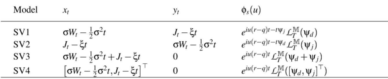
As mentioned earlier, to calculate option prices via equation (5), we need to know the characteristic exponents of the specified jump process. The three jump processes considered here (MJ, VG, and LS) all have analytical characteristic exponents, which we tabulate in Table I. We also include the characteristic exponent for the diffusion component for comparison. Given the L´evy measure πfor a particular jump process, we can derive the corresponding characteristic exponents using the L´evy-Khintchine formula (Bertoin (1996)),

ψj uL iub F D 0 1 e iux _iux1 M x MU 1 π dx

wherebdenotes a drift adjustment term.

Insert Table I About Here.

D. The Sources of Stochastic Volatility

The specification of a time-changed L´evy process given in equation (1) makes it transparent that stochastic volatility can come either from the instantaneous variance of the diffusion component or from the arrival rate of the jump component, or both. We consider four cases that exhaust the potential sources of stochastic volatility.

D.1. SV1: Stochastic Volatility from Diffusion

If we apply a stochastic time change to the Brownian motion only, i.e.,Wt WTd

t , and leave the

jump component Jt unchanged, stochastic volatility comes solely from the diffusion component. The

arrival rate of jumps remains constant. Examples using this specification include Bakshi, Cao, and Chen (1997) and Bates (1996). Under this specification, whenever the asset price movement becomes more volatile, it is due to an increase in the diffusive movements in the asset price. The frequency

of large events remains constant. Thus, the relative weight of the diffusion and jump components in the return process varies over time. The relative weight of the jump component declines as the total volatility of the return process increases.

D.2. SV2: Stochastic Volatility from Jump

Alternatively, if we apply a stochastic time change only to the jump component, i.e.,Jt JTj

t, but

leave the Brownian motion unchanged, stochastic volatility comes solely from the time variation in the arrival rate of jumps. Under this specification, an increase in the return volatility is due solely to an increase in the discontinuous movements (jumps) in the asset price. Hence, the relative weight of the jump component increases with the return volatility. The models proposed in Carr, Geman, Madan, and Yor (2003) are degenerate examples of this SV2 category because they apply stochastic time changes to pure jump L´evy processes.

D.3. SV3: Joint Contribution from Jump and Diffusion

To model the situation in which stochastic volatility comes simultaneously from both the diffusion and jump components, we can apply the same stochastic time change Tt (a scalar process) to both

Wt andJt. In this case, the instantaneous variance of the diffusion and the arrival rate of jumps vary

synchronously over time. Under SV3, the relative proportions of the diffusion and jump component are constant, even though the return volatility varies over time. The recent affine models in Bates (2000) and Pan (2002) are variations of this category. In these models, both the arrival rate of the Poisson jump and the instantaneous variance of the diffusion component are driven by one stochastic process.

D.4. SV4: Separate Contribution from Jump and Diffusion

The general specification is to apply separate time changes to the diffusion and jump components so that the time changeTt is a bivariate process. Under this specification, the instantaneous variance of the

diffusion component and the arrival rate of the jump component follow separate stochastic processes. Hence, variation in the return volatility can come from either or both of the two components. Since the two components vary separately over time, the relative proportion of each component also varies over

time. The relative dominance of one component over the other depends on the exact dynamics of the two activity rates. Specification SV4 encompasses all the previous three specifications (SV1-SV3) as special cases.

Under the affine framework of Duffie, Pan, and Singleton (2000), Bates (2000) also specifies a two-factor stochastic volatility process. Since each of the two volatility factors in Bates’s specification drives both a compound Poisson jump component and a diffusion component, his model can serve as a two-factor extension of our SV3 model. Alternatively, his model can also be regarded as a mixture of SV1 and SV3 specifications, since the intensity of the Poisson jump in the model includes both a constant term and a term proportional to the stochastic volatility factor (see also Andersen, Benzoni, and Lund (2002)). We can also see our SV4 specification as a special case of Bates’s specification if we set the diffusion component to zero in one factor and the jump component to zero in the other factor. Nevertheless, our separate treatment of the jump component and the diffusion component makes it easier to identify the different roles played by the two components.

We now derive the generalized Fourier transform of the log return for each of the four SV specifi-cations. Letxdenote the time-changed component andythe unchanged component in the log return, andψx andψy denote their respective characteristic exponents. We can write the generalized Fourier

transform of the log returnst ln

St S0 in equation (5) as φs u5 Z"[e iu1r2 q3t 8 yt8 xTt e iu1r2 q3t2 tψy > e 2 ψxT1t3 e iu1r2 q3t2 tψy

L

The complex-valued exponential martingale in equation (6) that defines the measure change becomes

dA d t exp iuyt iuxTt ψyt ψxTt

Table II summarizes thexand ycomponents, and the generalized Fourier transform of the log return, for each of the four SV specifications.

E. Specification of the Activity Rate Process

We finish our modeling by specifying an activity rate process v

t and deriving the Laplace

trans-form of the stochastic timeTt ]\

t

0v

sds under the new measure

A . Thus, we rewrite the Laplace

transform as

L

t as an instantaneous interest rate, equation (12) is analogous to the pricing formula

for a zero coupon bond. We can then borrow from the term structure of interest rates literature for the modeling of the activity rate. For example, we can model the activity rate of a Brownian motion after the term structure model of Cox, Ingersoll, and Ross (1985) and, in fact, recover the Heston (1993) stochastic volatility model. Multivariate activity rate processes can be modeled after affine models of Duffie and Kan (1996) and Duffie, Pan, and Singleton (2000), and the quadratic models of Leippold and Wu (2002).

Despite the large pool of candidate processes for the activity rate modeling, we leave the specifica-tion analysis of different activity rate models for future research. For the empirical work in this paper, we focus on one activity rate process, i.e., the Heston (1993) model. Under the risk-neutral measure ,

the activity rate process satisfies the following stochastic differential equation,

dv t κ 1 v t_ dt σv` v t dZt (13)

where Zt denotes a standard Brownian motion under , which can be correlated with the standard

Brownian motionWt in the return process byρdt a b" +dWtdZt/. Note that the long-run mean of the

activity rate is normalized to unity in equation (13) for identification purpose. For the SV4 specification, we assume that the two activity rates,v

tL $v d t v j t &

, follow a vector square-root process. Since the Laplace transform of the time change in equation (12) is defined under measure A , we

need to obtain the activity rate process under A . By Girsanov’s Theorem, under measure A , the

diffusion function ofv

t remains unchanged and the drift function is adjusted to

µ>ced fhg κ 1 v t_i iuσσvρv t forSV1SV3; κ 1 v t_i iuσσvρ ` v t forSV2

We call special attention to the difference between the drift adjustment for SV2 models and that for SV1 and SV3 models. This difference occurs because the diffusion component in the return process is time changed under all SV specifications except for the SV2 specification. Therefore, given that

dWTt

` v

t dWt holds in probability, the drift adjustment term for SV2 models is different from the

drift adjustment term for all other SV specifications by a scaling of ` v

t. The two-factor SV4 model

combines SV1 with SV2.

As the driftµ> remains affine for models SV1 and SV3 for anyρ

'

+

11

/, the arrival rate process

belongs to the affine class. The Laplace transform of Tt is then exponential-affine in v0 (the current level of the arrival rate), and is given by

L

For the SV2 specification, the affine structure is retained only whenρis zero. For tractability, we restrict ρto zero in our estimation of SV2 models. Under the SV4 model, we assume that the two activity rates are independent of each other and the activity rate for the diffusion component is correlated with the diffusion component in the return process. Then, the Laplace transform under the SV4 model becomes a product of two exponential affine forms, one for the SV1 component and the other for the SV2 component.

Substituting the Laplace transform in equation (14) into the generalized Fourier transforms in Table II, we can derive in analytical forms the generalized Fourier transforms for all 12 models: three jump specifications (MJ, VG, and LS) multiplied by four stochastic volatility specifications (SV1-SV4). We label these 12 models as “JJDSVn,” where JJ'ml MJVGLSn denotes the jump component, D refers to

the diffusion component, and SVn, withn 1

234, denotes a particular stochastic volatility

specifi-cation. For example, when the Merton jump diffusion model (MJD) is coupled with the SV1 specifica-tion, we have the model labeled as “MJDSV1.” This is the same specification as the one considered in Bakshi, Cao, and Chen (1997) and Bates (1996). Taken together, the 12 models are designed to answer two important questions: (1) What type of jump process performs best in capturing the behavior of S&P 500 index options? (2) Where does stochastic volatility come from?

III. Data and Estimation

We obtain from a major investment bank in New York daily closing bid and ask implied volatility quotes on the S&P 500 index options across different strikes and maturities from April 6, 1999 to May 31, 2000. The quotes are on standard European options on the S&P 500 spot index, listed at the Chicago Board of Options Exchange (CBOE). The implied volatility quotes are derived from out-of-the-money (OTM) option prices. The same data set also contains matching forward pricesF, spot prices (index levels)S, and interest ratesrcorresponding to each option quote, compiled by the same bank.

We apply the following filters to the data: that the time to maturity is greater than five business days; that the bid option price is strictly positive; and that the ask price is no less than the bid price. After applying these filters, we also plot the mid implied volatility quote for each day and maturity against strike prices to visually check for obvious outliers. After removing these outliers, we have 62,950 option quotes over a period of 290 business days.

Figure 1 shows in the left panel the histogram of moneyness of the cleaned-up option contracts, where the moneyness is defined ask ln

K S , withK being the strike price. The observations are

centered around at the money option contracts (k 0). On average, there are more OTM put option

quotes (kG 0) than OTM call option quotes (k

X 0), reflecting the difference in their respective trading

activities. The right panel of Figure 1 plots the histogram of the time-to-maturity for the option con-tracts. The maturities of the option contracts range from five business days to over one year and a half, with the number of option quotes declining almost monotonically as the time-to-maturity increases. These exchange-traded index options have fixed expiry dates, all of which fall on the Saturday follow-ing the third Friday of a month. The terminal payoff at expiry is computed based on the openfollow-ing index

level on that Friday. Thus, the contract stops trading on that expiring Thursday. To avoid potential microstructure effects, we delete from our sample the contracts that are within one week of expiry.

Insert Figure 1 About Here.

Since the FFT algorithm that we use returns option prices at fixed moneyness with equal intervals, we linearly interpolate across moneyness to obtain option prices at fixed moneyness. We also restrict our attentions to the more liquid options with moneynesskbetween 03988 and 01841. This

restric-tion excludes approximately 16 percent of the very deep out-of-money oprestric-tions (approximately eight percent each for calls and puts), which we deem as too illiquid to contain useful information. Note that we use an asymmetric moneyness range to reflect the fact that there are deeper out-of-the-money put option quotes than out-of-the-money call option quotes. Within this range, we sample options with a fixed moneyness interval of∆k 0

03068 (a maximum of 20 strike points at each maturity). For the

interpolation to work with sufficient precision, we require that at each day and maturity there be at least five option quotes. We also refrain from extrapolating: We only retain option prices at fixed moneyness intervals that are within the data range. Visual inspection indicates that at each date and maturity, the quotes are so close to each other along the moneyness line that interpolation can be done with little error, irrespective of the interpolation method. We delete one inactive day from the sample when the number of sample points is less than 20. The number of sample points in the other active 289 days ranges from 92 to 144, with an average of 118 sample points per day. In total, we have 34,361 sample data points for estimation.

We estimate the vector of model parameters,Θ, by minimizing the weighted sum of squared pricing errors, Θ arg min Θ T

∑

where

T

∑

∑

wherentqτandntqk denote, respectively, the number of maturities and the number of moneyness levels

per each maturity at datet,Nt denotes the total number of observations at datet,wi jdenotes an optimal

weight, andei jrepresents the pricing error at maturityiand moneyness j.

Note that there are two layers of estimation involved. First, given the set of model parameters Θ, we identify the instantaneous activity rates levelv

t at each datet by minimizing the weighted mean

squared pricing errors on that day. Next, we chooseΘto minimize the sum of the daily mean squared pricing errors.5 _{To construct out-of-sample tests, we divide the data into two subsamples: We use the} first 139 days of data to estimate the model parameters and then the remaining 150 days of data to test the models’ out-of-sample performance. To evaluate out-of-sample performance on the second subsample, we fix the parameter vectorΘestimated from the first sub-sample and compute the daily mean squared pricing errors according to equation (16): At each day, we choose the activity rate levels

v

t to minimize the sum of the weighted squared pricing errors on that day.

The pricing error matrixe

ei j is defined as e dr r r f r r r gts O Θ Oa if s O Θ X Oa 0 if Oa Y s O Θ Y Ob s O Θ Ob if s O ΘTG Ob (17) where s O

Θ denotes model-implied out-of-the-money option prices (put prices when K

Y F and call

prices whenKX F) as a function of the parameter vectorΘ, andOaandObdenote, respectively, the ask

and bid prices observed from the market. We set the pricing error to zero as long as the model implied price falls within the bid-ask spread of the market quote. We also normalize all prices as percentages of the underlying spot index level.

The construction of the pricing error is a delicate but important issue. For example, the pricing error can be defined with respect to implied volatility, call option price, or put option price. It can be defined as the difference in levels, in log levels, or in percentages. Here, we define the pricing error

using call option prices whenK X Fand put option prices whenKY F. This definition has become the

industry standard for several reasons, one of which is that in-the-money options have positive intrinsic value that is insensitive to model specification, but can still be the dominant component of the total option value. Another reason is that when there is a discrepancy between the market quotes on out-of-the-money options and their in-out-of-the-money counterparts, the former quotes are generally more reliable because they are more liquid. We refine the standard definition of the pricing error by incorporating the effects of the bid-ask spreads. Doing so reduces the potential problem of over-fitting and further accounts for the liquidity differences at different moneyness levels and maturities. Dumas, Fleming, Whaley (1998) also incorporate this bid-ask spread effect in their definition of “mean outside error.”

A. The Optimal Weighting Matrix

Like the definition of the pricing error, the construction of a “good” weighting matrix is also im-portant in obtaining robust estimates. Empirical studies often use identity weighting matrix. Under our definition of the pricing error, an identity weighting matrix puts more weight on near-the-money options than on deep out-of-the-money options. More important, it puts significantly more weight on long-term options than on short-term options. Thus, performance comparisons can be biased toward models that better capture the behavior of long-term options. Therefore, we want to estimate a weight-ing matrix that attaches a more balanced weightweight-ing to options at all moneyness and maturity levels, and which can be applied to the estimation and comparison of all relevant models.

One way to achieve this is to estimate an optimal weighting matrix based on the variance of the option prices, normalized as percentages of the underlying spot index level. We estimate the variance of the percentage option prices at each moneyness and maturity level via nonparametric regression and use its reciprocal as the weighting for the pricing error at that moneyness and maturity. This weighting matrix is optimal in the sense of maximum likelihood under the assumptions that the pricing errors are independently and normally distributed, and that the variance of the pricing error is well approximated by the variance of the corresponding option prices as percentages of the index level.

When the pricing errors are independently and normally distributed, if we set the weighting at each moneyness and maturity level to the reciprocal of the variance estimate of the pricing error at

that moneyness and maturity, the minimization problem in equation (15) also generates the maximum likelihood estimates. In principle, we can estimate the variance of the pricing errors via a two-stage procedure analogous to a two-stage least square procedure. However, the weighting obtained from such a procedure depends on the exact model being estimated. We use the variance of the option price (as a percentage of the index level) as an approximate measure for the variance of the pricing error. This approximation is exact when the return to the underlying stock index follows a L´evy process without stochastic volatility because for such processes the conditional return distribution over a fixed horizon does not vary over time. As a result, for a given option maturity and moneyness, the option price normalized by the underlying index level does not vary with time either. We can then estimate the “true” option price as a percentage of the index level through a sample average, and can consider the daily deviations from such a sample average as the pricing error. Therefore, the variance of the pricing error is equivalent to the variance of the option prices normalized by the index level.

However, all our model specifications incorporate some type of stochastic volatility. Thus, the variance of the option prices includes both the variance of the pricing error and the variation induced by stochastic volatility. Therefore, in our case the variance estimate of the option price is only an approximate measure of the variance of the pricing error. Nevertheless, our posterior analysis of the pricing errors confirms that such a choice of weighting matrix is reasonable. The idea of choosing a common metric, to which different and potentially non-nested models can be compared, is also used in the distance metric proposed by Hansen and Jagannathan (1997) for evaluating different stochastic discount factor models.

Since the moneyness and maturity of the options vary every day, we estimate the mean option value and the option price variance as percentages of the index level at fixed moneyness and maturities through a nonparametric smoothing method. The Appendix contains details for this estimation.

The left panel of Figure 2 shows the smoothed mean surface of out-of-the-money option prices. As expected, option prices are the highest for at-the-money options and they also increase with maturities. The right panel illustrates the variance estimates of the option prices. Overall, the variance increases with the maturity of the option. For the same maturity, out-of-the-money puts (k G 0) have a smaller

variation than do out-of-the-money calls (k X 0). This difference might be a reflection of different

calls. Given the estimated variance of the option prices, we define the optimal weight at each moneyness and maturity level as its reciprocal.

Insert Figure 2 About Here.

B. Performance Measures

We compare different models based on the sample properties of the daily mean squared pricing errors (mset) defined in equation (16) under the estimated model parameters. A small sample average

of the daily mean squared errors for a model would indicate that on average, the model fits the option prices well. A small standard deviation for a model would further indicate that the model is capable of capturing different cross-sectional properties of the option prices at different dates.

Our analysis is based on both the in-sample mean squared errors of the first 139 days and the out-of-sample mean squared errors of the last 150 days. We also gauge the statistical significance of the performance difference between any two modelsiand jbased on the followingt-statistic of the sample differences in daily mean squared errors:

t-statistic msei mse j stdev msei mse j (18)

where the overline on mse denotes the sample average and stdev

- denotes the standard error of the

sample mean difference. We adjust the standard error calculation for serial dependence based on Newey and West (1987), with the number of lags optimally chosen based on Andrews (1991) and an AR(1) specification.

IV. Model Performance Analysis

We analyze the parameter estimates and the sample properties of the mean squared pricing errors for each of the 12 models introduced in Section II. As mentioned earlier, our objective is to investigate

which jump type and which stochastic volatility specification perform the best in pricing S&P 500 index options. Our analysis below focuses on answering these two questions.

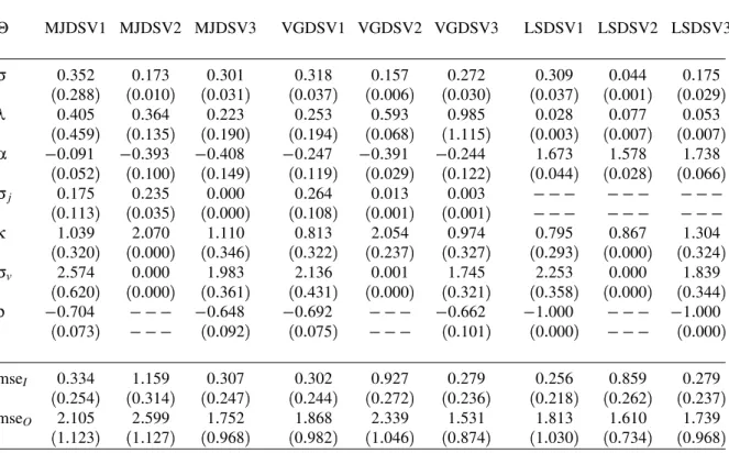
Tables III and IV report the parameter estimates and their standard errors for one-factor (SV1 to SV3) and two-factor stochastic volatility (SV4) models, respectively. In the tables we also report the sample average and standard deviation of the daily mean squared pricing errors, both in-sample (mseI)

and out-of-sample (mseO). Table V reports thet-statistics defined in equation (18) for pair-wise model

comparisons. With 12 models, we could have reported a 12 u 12 matrix of pair-wiset-tests, but to

focus on the two questions raised above, we report thet-tests in two panels. Panel A compares the performance of different jump structures under each stochastic volatility specification (SV1 to SV4), and Panel B compares the performance of different SV specifications for a given jump structure (MJ, VG, or LS). The table reports both in-sample and out-of-sample comparisons.

Insert Table III About Here.

Insert Table IV About Here.

Insert Table V About Here.

A. What Jump Structure Best Captures the Behavior of S&P 500 Index Options?

Since our 12 models are combinations of three jump structures and four SV specifications, to an-swer the question raised on jump types, we compare the performance of the three jump structures under each SV specification. If the performance ranking of the three jump structures depends crucially on the specific SV specification, then the choice of a jump structure in model design should be contingent on which SV specification we use. On the other hand, if the performance rankings are the same under

each of the four SV specifications, then we would conclude that in capturing the behavior of S&P 500 index options, the superiority of one jump structure over the others is unconditional and robust to vari-ations in the SV specification. The empirical evidence matches the latter scenario. The infinite activity jump structures (VG and LS) outperform the traditional finite activity compound Poisson (MJ) jump structure under all four SV specifications.

Panel A of Table V addresses the question based on thet-statistics defined in equation (18). Each column in Panel A compares the performance of two jump structures under each SV specification. For example, the column “MJ-VG” compares the performance of the Merton jump model (MJ) against the performance of the variance-gamma model (VG), under each of the four SV specifications. At -statistics of 1.645 or higher implies that the pricing error from the MJ model is significantly larger than the pricing error from the VG model under a 95 percent confidence interval. Therefore, the VG model outperforms the MJ model. At-value of 1645 or less implies the opposite.

The in-samplet-values in column “MJ-VG” are strongly positive under all SV specifications, so are all the in-samplet-values in the “MJ-LS” column. The out-of-sample tests reveal similar results, except for the SV4 case. Therefore, our test results indicate that out of the three jump structures, the most commonly used compound Poisson jump structure of Merton (1976) performs significantly worse than both the VG and the LS jump structures. This result holds under all of the four SV specifications and for both in-sample and most of the out-of-sample tests.

On the other hand, the performance difference between VG and LS is much smaller and can have different signs, depending on the SV specification assumed. Thet-values in the “VG-LS” column are much smaller, positive under SV1 and SV2, but negative under SV3 and SV4. Carr and Wu (2003a) obtain similar performance rankings for the three jump structures without incorporating any stochas-tic volatilities. Our results show that this ranking remains unchanged in the presence of stochasstochas-tic volatility.

The key structural difference between the Merton jump model and the other two types of jump structures lies in the jump frequency specification. Within any finite time interval, the number of jumps under MJ is finite and is captured by the jump intensity measureλ. Under the MJ structure, the estimates forλfall between 0178 under the SV4 specification (see Table IV) and 0405 under the SV1

specification (see Table III). An estimate of 0405 or smaller implies about one jump every two and

half years, a rare event. In contrast, under the VG and LS jump structures, the number of jumps within any finite time interval is infinite. Therefore, we can expect to observe much more frequent jumps of different magnitudes than in the Merton jump case. Our estimation results indicate that to capture the behavior of S&P 500 index options, we need to incorporate a much more frequent jump structure in the underlying return process than the classic Merton model allows.

B. Where Does Stochastic Volatility Come From?

By applying stochastic time change to different L´evy components, we can generate stochastic volatility from either the diffusion component, or the jump component, or both. Thus, it becomes a purely empirical issue as to where, exactly, the stochastic volatility comes from. We address this issue by comparing the empirical performance of four different stochastic volatility specifications in pricing the S&P 500 index options.

In Table V, Panel B compares the performance of the four stochastic volatility specifications under each of the three jump structures. We first look at the three one-factor SV specifications, SV1, SV2, and SV3. We find that the in-samplet-test values in the “SV1-SV2” column are all strongly negative and the in-samplet-test values in the “SV2-SV3” column are all strongly positive, which suggests that the SV2 specification is significantly outperformed by the other two one-factor SV specifications. In contrast, the in-samplet-test estimates in the “SV1-SV3” column are much smaller and have different signs under different jump specifications, positive under MJ and VG, negative under LS. The out-of-sample performance comparison gives similar conclusions, except under the LS jump structure where thet-statistics are much smaller.

Under the SV2 specification, the instantaneous variance of the diffusion component is constant and all stochastic volatilities are attributed to the time variation in the arrival rate of jumps. The inferior performance of SV2, as compared to SV1 and SV3, indicates that the instantaneous variance of the diffusion component should be stochastic. The parameter estimates of the three one-factor SV speci-fications in Table III tell a similar story. The volatility of volatility estimates (σv) are always strongly

SV2 specifications, when only the arrival rate of the jump component is allowed to be stochastic. For example, the estimate ofσv is 2.136 under VGDSV1, 1745 under VGDSV3, but a mere 0001 under

VGDSV2. Similar results hold for the MJ and LS models. These estimates indicate that the arrival rate of the jump component is not as volatile as the instantaneous variance of the diffusion component. This evidence supports traditional stochastic volatility specifications, but casts doubt on the performance of the stochastic volatility models of Carr, Geman, Madan, and Yor (2003), which generate stochastic volatility from pure jump models.

Another important structural difference between the SV2 specification and the other SV specifica-tions is that SV2 is the only specification in which instantaneous correlation is not incorporated between the return innovation and the innovation in the activity rate. Therefore, the SV2 specification cannot capture the widely documented negative correlation between stock returns and return volatilities, i.e., the “leverage effect.”6 _{Yet, under all other SV specifications, the estimates for this instantaneous} cor-relation parameterρare strongly negative (see Table III), suggesting the importance of incorporating such a leverage effect in capturing the behavior of S&P 500 index option prices. This negative correla-tion helps generate negative skewness in the condicorrela-tional index return distribucorrela-tion implied by the opcorrela-tion prices.

Consistent with our observation, Carr, Geman, Madan, and Yor (2003) also note that without the leverage effect, the performance of the SV3 specification declines to approximately the same level as that of the SV2 specification. Therefore, this lack of negative correlation under SV2 constitutes another key reason for its significantly worse performance compared to other one-factor SV specifications.

In contrast to the three one-factor SV specifications, the SV4 specification allows the instantaneous variance of the diffusion component and the arrival rate of the jump component to vary separately. The

t-statistics in Table V indicate that this extra flexibility significantly improves the model performance. The t-tests for performance comparisons between SV4 and all the one-factor SV specifications are strongly negative both in-sample and out-of-sample, which indicates that the two-factor SV4 models perform much better than all the one-factor SV models. This superior performance of the SV4 models indicates that stochastic volatility actually comes from two separate sources, the instantaneous variance of the diffusion component and the arrival rate of the jump component.

The superior performance of the SV4 models implies that a high-volatility day on the market can come from either the intensified arrival of large events or the increased arrival of small, diffusive events, or both. Therefore, the exact source of high volatility is subject to further research and shall be case dependent. This result contrasts with the implication of earlier option pricing models, e.g., Bates (1996) and Bakshi, Cao, and Chen (1997), both of which assume that variations in volatility can only come from variations in the diffusive volatility.

C. How Do the Risk-Neutral Dynamics of the Two Activity Rates Differ?

Since the SV4 specification provides a framework that encompasses all the one-factor SV speci-fications, we can learn more about the risk-neutral dynamics of the activity rates by investigating the relevant parameter estimates of the SV4 models, which are reported in Table IV.

Based on the square-root specification in equation (13) for the risk-neutral activity rate dynamics, the two elements of σv σ

d vσ

j

v capture the instantaneous volatility of the two activity rate

pro-cesses, withσd

v capturing the instantaneous volatility of the diffusion variance andσvjthe instantaneous

volatility of the jump arrival rate. The estimates indicate that the variance of the diffusion component shows larger instantaneous volatility than the arrival rate of the jump component. For example, the esti-mates forσd

v are 2.646, 2.555, and 2.856 when the jump components are MJ, VG, and LS, respectively.

In contrast, the corresponding estimates for σvj are 2.313, 1.428, and 1.148, evidently lower than the

corresponding estimates forσd v.

On the other hand, the relative persistence of the activity rate dynamics is captured by the two elements of κ $κ

d

κ

j&

. A smaller value for κimplies a more persistent process. The estimates reported in Table IV indicate that the arrival rate of the jump component exhibits much more persistent risk-neutral dynamics than the instantaneous variance of the diffusion component. The estimates forκj

are 0.001, 0.63, and 0.668, when the jump components are MJ, VG, and LS, respectively, much smaller than the corresponding estimates forκd_{, which are 1.872, 1.898, and 2.119, respectively.}

The parameter estimates for the SV4 specifications indicate that to match the market price behav-ior of S&P 500 index options, we need to derive stochastic volatilities from two separate sources, the instantaneous variance of the diffusion component and the arrival rate of the jump component.

Fur-thermore, the risk-neutral dynamics of the diffusion variance exhibits higher instantaneous volatility and much less persistence than the neutral dynamics of the jump arrival rate. Such different risk-neutral dynamics for the two activity rate processes dictate that the jump and diffusion components play different roles in governing the behavior of S&P 500 options. The more volatile, but also more transient, feature of the activity rate from the diffusion component implies that the variation of the diffusion component is more likely to dominate the price behavior of the short-term options. On the other hand, although the activity rate from the jump component is not as volatile, its highly persistent nature implies that its impact is more likely to last longer and hence dominate the behavior of long-term options. These different impacts generate potentially testable implications on the time series behavior of S&P 500 index options.

D. Shall We Take the Diffusion Component for Granted?

One consensus in the option pricing literature is that to account for the pricing biases in the Black-Scholes model, we need to add both a jump component and stochastic volatility. This consensus im-plicitly takes for granted the Brownian motion component in the Black-Scholes model. This view is not surprising since most of the jump models in the literature are variations of Merton’s finite activity compound Poisson jump model. In these models, the number of jumps within a finite interval is finite. For example, under the MJDSV1 model, our estimate for the Poisson intensity is 0405 (Table III),

which implies an approximate average of one jump every two and half years. Obviously, we need to add a diffusion component to fill the gaps between the very infrequent jumps in the asset price process. However, if we consider jump processes with infinite activity, or even infinite variation, the infinite small jumps generated from such models can fill these gaps. Carr, Geman, Madan, and Yor (2002) conclude from their empirical study that a diffusion component is no longer necessary as long as they adopt an infinite activity pure jump process. Carr and Wu (2003a) arrive at similar conclusions in their infinite variation log stable (LS) model. Carr and Wu (2003c) identify the presence of jump and diffusion components in the underlying asset price process by investigating the short-maturity behavior of at-the-money and out-of-the-money options written on this asset. They prove that a jump component, if present, dominates the short-maturity behavior of out-of-the-money options and hence can readily be identified. A diffusion component, if present, usually dominates the short-maturity behavior of

at-the-money options. Nevertheless, they find that in theory, an infinite-variation jump component can also generate the same short-maturity behavior for at-the-money options as does a diffusion process. The same infinite variation feature for both a Brownian motion and an infinite-variation pure jump process implies that they generate similar short-maturity behaviors for at-the-money options.

These empirical and theoretical findings lead us to ask questions beyond the traditional framework of thinking: Do we really need a diffusion component if we include an infinite-activity jump component in the option pricing model? Can we separately identify a diffusion component from an infinite-activity jump component, especially one that also shows infinite variation? These questions are especially relevant here, since our estimation results strongly favor the infinite activity jump components, and the infinite variation LS jump component in particular, over the more traditional finite activity compound Poisson MJ jump specification.

Tables III and IV show that under all the tested models with infinite-activity jump components (VG or LS), the estimates for the diffusion parameterσare all significantly different from zero. This finding indicates that the diffusion component is both identifiable and needed. The key difference between our models and those estimated in Carr, Geman, Madan, and Yor (2002) and Carr and Wu (2003a) is that we incorporate stochastic volatility, but they consider pure L´evy processes without stochastic volatility. Thus, our identification of the diffusion component comes from its role in generating stochastic volatil-ity. The separate specification of the two activity rate processes under SV4 implies that the relative proportion of small (diffusive) movements and large (jump) movements can vary over time. Their dif-ferent risk-neutral dynamics further imply that the two components can separately dominate the price behaviors of options at different maturities.

Furthermore, our empirical work focuses on a purely diffusive specification for the activity rate pro-cess, i.e., the Heston (1993) model. Under such a specification, any instantaneous negative correlation between the activity rate process and the return innovation must be incorporated by using a diffusion component in the return process, because a pure jump component is by definition orthogonal to any diffusion components. Thus, under our specification, the diffusion component in the return process is not only important in providing a separate source of stochastic volatility, but also indispensable in providing a vehicle to accommodate the leverage effect. We can conceivably incorporate a jump com-ponent in the activity rate process, as in Chernov, Gallant, Ghysels, and Tauchen (1999) and Eraker,

Johannes, and Polson (2003). Doing so would allow us to accommodate the leverage effect via a cor-relation between the jump component in the return process and the jump component in the activity rate processes. When these two jump components exhibit infinite variation, the need for a separate diffusion component could be reduced.

Even under our diffusive activity-rate specification, the model parameter estimates indicate that the relative proportion of the diffusion component declines as the jump specification goes from finite activity (MJ) to infinite activity but finite variation (VG), and to infinite variation (LS). Given that we calibrate all models to the same data set, the estimate of the diffusion parameterσrepresents the relative weight of the diffusion component compared to the jump component. The decline in the relative weight of the diffusion component holds for all SV specifications. For instance, among the SV4 models shown in Table IV, the estimate of σ(the diffusion parameter) is 0312 for MJDSV4, 0310 for VGDSV4,

but 0308 for LSDSV4. We observe similar declines under SV1 specifications (from 0.352, to 0.318,

and then to 0.309) and SV3 specifications (from 0.301, to 0.272, and then to 0.175). However, the most dramatic decline comes under the SV2 specification. The estimate forσis 0.173 under MJDSV2, 0.157 under VGDSV2, but a meager 0.044 under LSDSV2. SV2 differs from all other SV specifica-tions in generating stochastic volatility from the jump component only and by not accommodating a leverage effect. Thus, consistent with our discussion above, without a role in either generating stochas-tic volatility or accommodating a leverage effect, the diffusion component is hardly needed when the jump component also shows infinite variation, as in the case of LSDSV2.

Combining all the evidence, we conclude that as the frequency of jump arrival increases from MJ to VG and then to LS, the need for a diffusion component declines. The many small jumps in infinite variation jump components can partially replace the role played by a diffusion component. Neverthe-less, under our specifications, the diffusion component plays important roles in providing a separate source of stochastic volatility and accommodating the leverage effect between the return innovation and the activity rate process. Therefore, under our specifications, the diffusion component cannot be totally replaced by the jump component, even if the jump component exhibits infinite variation.