Open PRAIRIE: Open Public Research Access Institutional
Open PRAIRIE: Open Public Research Access Institutional
Repository and Information Exchange
Repository and Information Exchange
Electronic Theses and Dissertations2019
Multi-Step Forecast of the Implied Volatility Surface Using Deep
Multi-Step Forecast of the Implied Volatility Surface Using Deep
Learning
Learning
Nikita Medvedev
South Dakota State University
Follow this and additional works at: https://openprairie.sdstate.edu/etd
Part of the Finance Commons Recommended Citation
Recommended Citation
Medvedev, Nikita, "Multi-Step Forecast of the Implied Volatility Surface Using Deep Learning" (2019). Electronic Theses and Dissertations. 3647.
https://openprairie.sdstate.edu/etd/3647
This Thesis - Open Access is brought to you for free and open access by Open PRAIRIE: Open Public Research Access Institutional Repository and Information Exchange. It has been accepted for inclusion in Electronic Theses and Dissertations by an authorized administrator of Open PRAIRIE: Open Public Research Access Institutional Repository and Information Exchange. For more information, please contact [email protected].
BY
NIKITA MEDVEDEV
A thesis submitted in partial fulfilment of the requirements for the Master of Science
Major in Economics South Dakota State University
2019 LEARNING
THESIS ACCEPTANCE PAGE
This thesis is approved as a creditable and independent investigation by a candidate for the master’s degree and is acceptable for meeting the thesis requirements for this degree. Acceptance of this does not imply that the conclusions reached by the candidate are necessarily the conclusions of the major department.
Advisor Date
Department Head Date
Dean, Graduate School Date
Nikita Medvedev
Zhiguang Wang
ACKNOWLEDGMENTS
I want to express my sincere gratitude to my advisor, Dr. Zhiguang Wang, for his support, encouragement, and patience throughout my graduate studies. I appreciate his guidance and expertise in the areas of finance, statistics, and financial derivatives that were indispensable for the completion of this thesis. His passion for excellence inspires me to challenge myself and keep learning. My thanks also go to Dr. Matthew Diersen for providing valuable guidance and insightful comments that improved the contents of this thesis.
I want to thank the Ness School of Management and Economics for funding my graduate studies and providing me with many opportunities for expanding my knowledge in finance and economics, both domestically and internationally. I am thankful to EV Technologies Inc. for helping me gain the necessary data analytics experience for completing this research.
Finally, I would like to thank my father, Juri Medvedev, and my mother, Jelena Medvedeva, for their continuous support, assistance, and encouragement during my undergraduate and graduate studies.
CONTENTS
LIST OF FIGURES . . . vi
LIST OF TABLES . . . vii
ABSTRACT . . . viii 1 INTRODUCTION . . . 1 1.1 BACKGROUND . . . 1 1.2 PROBLEM . . . 1 1.3 PRELIMINARIES . . . 3 1.4 GOAL . . . 6 2 LITERATURE REVIEW . . . 6 2.1 IMPLIED VOLATILITY . . . 7
2.2 HISTORICAL VOLATILITY FORECASTING . . . 9
2.3 IMPLIED VOLATILITY FORECASTING . . . 11
3 DATA AND METHODOLOGY . . . 12
3.1 DATA DESCRIPTION . . . 12
3.2 DATA PREPARATION . . . 13
3.3 BS PDE SOLVER . . . 16
3.4 IV LOG-MONEYNESS BINNING . . . 17
3.5 STATIONARITY AND COINTEGRATION TESTS . . . 18
3.6 FORECASTING MODELS . . . 24
3.6.1 LONG-SHORT TERM MEMORY MODEL . . . 24
3.6.2 CONVOLUTIONAL LONG-SHORT TERM MEMORY MODEL 26 3.6.3 VECTOR AUTOREGRESSION MODEL . . . 28
4 ALGORITHMS AND OPTIMIZATIONS . . . 29
5 RESULTS AND DISCUSSION . . . 33
5.1 MODEL EVALUATION CRITERIA . . . 33
5.2 RESULTS . . . 35
5.3 CONCLUSION . . . 46
APPENDIX . . . 49
A STATISTICAL RESULTS . . . 49
LIST OF FIGURES
1 Average interpolated Implied Volatility Surface (IVS) between 2007-08-17 and 2007-12-31. . . 2 2 Selected at-the-money (ATM) IV for March, June, September and
De-cember contracts and expirations. . . 13 3 ADF Test for 2002-2007. . . 20 4 KPSS Test for 2002-2007. . . 21 5 Simple RNN cell and LSTM memeory cell as presented in Greff et
al. (2017). . . 25 6 LSTM and ConvLSTM model flowcharts. . . 26 7 Forecasting ConvLSTM as presented in Shi et al. (2015). . . 27 8 LSTM (blue) vs ConvLSTM (orange) training process with minimizing
scaled IV MSE. . . 32 9 Average out-of-sample predicted IV. . . 37 10 Average out-of-sample predicted Savitzky-Golay smoothed IV. . . 38 11 Average and predicted IVS for the 90 day out-of-sample period . . . . 40 12 Average IV residual for the 90 day out-of-sample period. . . 41
LIST OF TABLES
1 Descriptive statistics of implied volatility observations. . . 15 2 Johansen test trace statistic critical values. . . 23 3 Mean in-sample performance, mean out-of-sample performance and
Savitzky-Golay filter smoothed prediction performance on the out-of-sample set. . . 35 4 Mean out-of-sample RMSE and MAPE grouped by expiration month
and contract type. . . 35 5 Average out-of-sample forecast, for 1-day, 30-day, 60-day, and 90-day
horizons. . . 36 6 DM Test for 1, 30, 90 trading day horizon. . . 44 7 LSTM forecast vs VEC forecast Welch’s significance tests . . . 49 8 ConvLSTM forecast vs VEC forecast Welch’s significance tests . . . . 52 9 ConvLSTM forecast vs LSTM forecast Welch’s significance tests . . . 55
ABSTRACT
MULTI-STEP FORECAST OF THE IMPLIED VOLATILITY SURFACE USING DEEP LEARNING
NIKITA MEDVEDEV 2019
Implied volatility is an essential input to price an option. Machine learning architectures have shown strengths in learning option pricing formulas and estimating implied volatility cross-sectionally. However, implied volatility time series forecasting is typically done using the univariate time series and often for short intervals. When a univariate implied volatility series is forecasted, important implied volatility properties such as volatility skew and the term structure are lost. More importantly, short term forecasts can’t take advantage of the long term persistence in the volatility series.
The thesis attempts to bridge the gap between machine learning-based implied volatility modeling and multivariate multi-step implied volatility forecasting. The thesis contributes to the literature by modeling the entire implied volatility surface (IVS) using recurrent neural network architectures. I implement Convolutional Long Short Term Memory Neural Network (ConvLSTM) to produce multivariate and multi-step forecasts of the S&P 500 implied volatility surface. The ConvLSTM model is capable of
understanding the spatiotemporal relationships between strikes and maturities (term structure), and of modeling volatility surface dynamics non-parametrically.
I benchmark the ConvLSTM model against traditional multivariate time series Vector autoregression (VAR), Vector Error Correction (VEC) model, and deep
learning-based Long-Short-Term Memory (LSTM) neural network. I find that the ConvLSTM significantly outperforms traditional time series models, as well as the benchmark Long Short Term Memory(LSTM) model in predicting the implied volatility surface for a 1-day, 30-day, and 90-day horizon, for out-of-the-money and at-the-money calls and puts.
1 INTRODUCTION
1.1 BACKGROUND
The typical performance of a financial asset is measured via its return. The fluctuations in the returns, as well as their randomness, is described by the asset’s volatility. Volatility modeling has been extensively researched in the areas of finance, risk management, and policymaking. Volatility is an essential component of financial derivatives; models and forecasts are particularly important for the institutions involved in derivative trading. Good forecasts of the volatility of asset returns enable institutions to asses their investment risk and optimize their investment portfolios. Two measures of volatilities exist: 1)
historical (realized) volatility, which can be observed from the historical data and realized at a certain point in time; 2) implied volatility (IV), which is not directly observable, but instead is an investor’s forward-looking view on the underlying asset’s future returns. Market expectations, macroeconomic conditions, and general market supply and demand are common factors that drive future volatility. Implied volatility is typically derived through a closed-form formula. Changes in implied volatility are market-driven and dynamic, which makes predicting future implied volatility a challenging task.
1.2 PROBLEM
As identified in the survey by Samsudin and Mohamad (2016), the vast majority of volatility forecasting models fall into two major categories: 1) option-implied volatility models and 2) historical time series models. The former represents traders’
forward-looking view on the future direction of an asset’s volatility throughout the life-cycle of the contract. Because the market attempts to predict the future expected volatility of the underlying asset that changes dynamically, the incorrect parameters to the closed-form option pricing formula lead to a degree of overpricing of the options as the time to maturity of the contract increases (Hull and White, 1987). On the other hand,
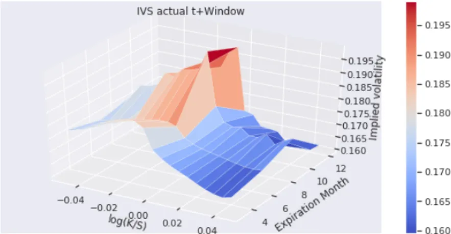
Figure 1: Average interpolated Implied Volatility Surface (IVS) between 2007-08-17 and 2007-12-31.
historical time series tries to express future price trends relying on past price trends. This approach doesn’t take into consideration the market’s expectations of future returns. Likewise, time series methods tend to ignore the underlying asset’s fundamental information, such as earnings, debt, revenues, or other news.
Implied volatility (IV) has two important empirically observed properties: 1) IV term structure; 2) IV skew. The first property implies that the future IV is typically higher than today’s IV because of the large degree of uncertainty in future returns. The second property implies that the market sentiment and investor preferences can cause option strikes to have differences in IV levels. The voluminous literature has popularized the Skew following empirical studies such as Rubinstein (1985), Dupire (1994), and Dumas, Fleming, and Whaley (1998) that collectively bring out that IV’s vary with strike prices and time-to-maturities, in contrast with the assumptions of the (Black and Scholes, 1973) option pricing model (BSM), which assumes constant volatility and log-normal price distribution of the underlying asset. IV skew and IV term structure can be captured in a dynamic 3D figure known as the implied volatility surface (IVS). In the short term, deviations, from the classical IVS shape can be observed, such as upward skew for some strikes, or downward term structure. For instance, in Figure 1 between 2007-08-17 and 2007-12-31, it is observed that the IV is higher for OTM puts than OTM calls and that IVS
has a downward IV term structure. Much of the previous research on option-implied volatility modeling and forecasting focuses on producing cross-sectional results spearheaded by the non-parametric methods for volatility pricing and not time series forecasting. This is an area where machine learning architectures have shown significant strengths. Adaptation of these data-driven machine learning techniques in volatility research tends to focus on three major areas: 1) forecasting future historical volatility of an underlying asset; 2) non-parametric framework or solvers for option or pricing; 3) time series forecasting on the option implied volatility, volatility products (e.g., VIX), or volatility distributions. The term structure dimension used to be a secondary priority for earlier researchers but is thoroughly addressed in the more modern research
(Chalamandaris and Tsekrekos, 2011). The thesis contributes to the third major subsection of the literature that focuses on implied volatility forecasting and proposes a data-driven machine learning technique for pricing IV and multi-step forecast of both IV skew and IV term structure through the IVS.
1.3 PRELIMINARIES
Forecasting historical volatility means predicting future volatility using historical
volatility. A number of studies had been conducted over the years using the financial time series or econometric models to address this. One of the assumptions of a typical
regression model is constant variance (random noise) of the residuals, also known as homoscedasticity. However, it is well known that financial time series tend to experience unequal differences in means, medians, and interquartile ranges across different periods, and thus, the residuals follow a mixture of distributions, also known as heteroscedasticity. Up until more recent years, autoregressive conditional heteroscedasticity (ARCH) model (Engle, 1982) where the lagged variance of the series is expressed as a function of time, and generalized autoregressive conditional heteroscedasticity (GARCH) family models (Bollerslev, 1986), were among the best models in forecasting realized volatility.
However, GARCH family models tend to produce a term structure that reverts to the long-term mean (Sinclair, 2013) and fails to capture the volatility skew (Dupire, 1994). Throughout the years, many GARCH family models have evolved to address the failure of capturing the IV skew. However, Hansen and Lunde (2005), tested over 330 GARCH family models, seeking to identify advantages of the more sophisticated models to a standard GARCH(1,1) model. The research found no evidence that more sophisticated GARCH models significantly outperform the standard GARCH(1,1) model.
The results of a number of empirical studies suggest that option-implied volatility can be used to predict future volatility. Time series predictions of IV can outperform historical volatility (HV) as a predictor of future realized volatility (RV) (Samsudin and Mohamad, 2016; Chalamandaris and Tsekrekos, 2011). More-so forecasted IV and historical IV are more closely related than RV and IV, and the conditions in the options market can impact this relationship (Zumbach, 2009). More recently, studies had emerged that utilize a hybrid approach by combining various iterations of neural networks with GARCH models, specifically to address the relative weakness of capturing the IV skew. Neural networks have shown advantages in estimating complex non-linear functions, which is often achieved through the depth of the networks, number of neurons, and the activation (transfer) functions between the layers, and given a suitable degree of
complexity can be trained to estimate any non-parametric function. This, however, comes at a higher performance cost and a lengthy training process. However, the rise of the new data warehousing techniques, as well as high-performance computing in the 1990s, kick-started a new branch of non-parametric financial derivative research that
predominantly focuses on providing efficient solutions to the partial differential equations (PDEs). Often the use of the non-parametric algorithms and techniques, such as forests, boosting, support vectors, and neural networks for volatility estimation can lead to far more superior results (Park, Kim, and Lee, 2014). The usage of the artificial neural networks (ANNs) primarily focuses on development of efficient alternatives to the time
consuming numerical solvers which fail to deliver fast on-line solutions (Liu, Oosterlee, and Bohte, 2019). Because of this performance bottleneck, the ANNs are trained to approximate the PDEs. The solutions are expressed as a set of matrix multiplication, and the workload distributed to the graphical processing units (GPUs) and run in parallel, which significantly improves the computational performance. Multiple researchers have noted significant performance gains from applying these techniques to the widely recognized options pricing models. Culkin and Das (2017) applied the simplest form of ANN, multi-layer perceptron (MLP) neural network to the BSM option pricing model. They note that deep neural networks can serve as a universal approximator for almost any function. In particular, the results were significant when applied to the BSM model. Liu, Oosterlee, and Bohte (2019) did the same for both BSM and Heston stochastic volatility (Heston, 1993) models, which confirmed the findings of Culkin and Das (2017).
The IV skew and the term structure can be captured in the implied volatility surface (IVS). The IVS is used by the market participants to price the options. However, because option volume is supply and demand-driven, markets often do not have quotes for all of the strikes and maturities, so the IVS is interpolated to fill the missing quotes
(Orosi, 2012), which is why forecasting and interpolation techniques are especially important for the market makers. For example, CBOE’s Volatility Index (VIX) is a measure of expected annualized volatility implied by S&P 500 options that are measured and published by the Chicago Board of Exchange (CBOE). The VIX itself is a measure derived from the near term SPX option contract. VIX, due to its popularity, has been a research topic of many studies. Traders consider VIX a mean-reverting asset, and thus a variation of mean-reverting time series models (e.g., GARCH family) seems to be a natural choice for a large number of studies for forecasting VIX. Although the calculation of the VIX is transparent, the spot VIX is difficult to replicate because of the square root function. So because of the difficulty to replicate VIX and VIX covering only the near term contract, the forecast of the IVS from a traders perspective is of great importance.
1.4 GOAL
Neural networks can learn IV equations accurately, and parametric time series models are able to capture temporal relationships. The thesis bridges the gap between these two methodologies by applying two new neural network architectures for multi-step time series forecasting of the IVS that also takes advantage of non-parametrically learned BS-IV function. The thesis contributes to the literature of modeling and forecasting implied volatility using entirely machine learning techniques. The goal of this thesis is to answer three overarching research questions: 1) Do the cointegrated relationships
significantly impact the multi-step forecast of the IVS? Cointegration is relevant because of the short-run stochastic dynamics of volatility; 2) Can the recurrent neural network architecture significantly outperform traditional time series models in a multi-step out-of-sample forecast of the IVS? While MLP’s have shown strength in option pricing and volatility estimation, supervised time-series predictions are computationally
expensive; 3) Does encoding spatiotemporal dynamics of the IVS significantly improve the IVS forecasts? All traditional time series forecasting models require flattening of the data input vector - this loses the important properties of the IV term structure and the IV skew. Lastly, I will select the IVS forecasting methodology with the lowest forecasting error for multiple time horizons. I aim to demonstrate that the combination of these factors can lead to an overall improvement in forecasting the option based implied volatility over the traditional time series approaches.
2 LITERATURE REVIEW
In this section, I will briefly discuss the geometric Brownian motion (GBM), which is a core component of three widely popular option pricing models. I discuss the
Black-Scholes model and briefly mention other methods for option pricing and implied volatility modeling. I will also review econometric and parametric methods that are
relevant for volatility time-series forecasting. Lastly, I will review some of the more recent methodologies used for option implied volatility forecasting and option pricing, with the help of traditional Artificial Neural Networks and more recent deep learning architectures.
2.1 IMPLIED VOLATILITY
The BS model (Black and Scholes, 1973) undoubtedly had a significant impact on the world of finance and provided a theoretical framework for options trading and hedging. One of the main advantages of the model is that the BS formula can be inverted to produce implied volatility and IVS.
The key underlying assumption of the model is that an underlying asset follows the stochastic processStsuch that:
dSt=µStdt+σStdWt (1)
where bothµor the drift andσvolatility are constant andWtis a Brownian motion. Using
Ito’s lemma, the BS equation for the European call option can be denoted as:
∂C ∂t + 1 2σ 2S2∂2C ∂C2 + rS ∂C ∂S = rC (2)
wheretis time to maturity, risk-free rate isr. The Equation 2 serves as a closed form solution for pricing European call and put options:
C(S,t) = N(d1)S−N(d2)Ke−rt d1 = 1 σ√t ln S K +t r+σ 2 2 d2 =d1−σ √ t N(x) = √1 2π Z x −∞ e−12z 2 dz (3)
Although BS makes assumptions on the underlying asset that don’t hold
empirically such as log return of stock price with constant volatility it’s still an incredibly useful and almost a universally used mechanism for extracting IV given the option market data (Homescu, 2011).
σ(K, t) = BS−1(C, S, K, t, r) (4)
BS volatilityσcan be derived by solving Equation 4, whereBS−1denotes inverse BS function. The inverse Equation 4 can be solved numerically, with an iterative technique that solves Newton-Raphson formula, since BS equation guaranteesσsuch that
σ ∈[0,∞]1: solve forσ imp: σimp =σn− BS(σn)−P ν(σn) (5)
whereσimpis the IV,P is option price,vis the volatility derivative vega. Initially an
arbitraryσ0 is guessed, and given the market data, the iterative solution will converge to the optimalσimp.2 The key limiting factor of the BS model is the constant volatility, which
fails to capture the skew (smile) present in the market data. Hull and White (1987) identified that BS model under-prices at-the-money options and overprices deep-out-of money options, and the effect is exaggerated as the time to maturity increases. Extensions to the BS model had been made to account for the smile effect, but one has to break the intuition behind Equation 2 that the options risk can be fully hedged by trading the underlying. This adds non-tradable risk sources such as jump risk, stochastic volatility, or transaction costs (Dupire, 1994; Eraker, Johannes, and Polson, 2003). Furthermore, volatility is strike dependent and it’s attributed to an option trader’s belief in leptokurtosis of an underlying asset and expectations of larger price swings than assumed by the GBM,
1BS(σ) for European options has a closed-form volatility derivative (vega) which is non-negative. 2Solution works well with European payoffs. Exotic payoffs require applying secant optimization method.
which would increase the market prices of the out-of-money options relative to the BS prices (Alexander, 2004). This is because of the risk premium caused by the changes in volatility (Heston, 1993).
Heston (1993) proposed a widely popular model that allows for a stochastic correlation between underlying asset returns and its volatility. The resulting two-factor stochastic volatility model (SV) can be used to explain the presence of the implied
volatility smile, especially in the long time to maturity options. The model is often used as a benchmark for other option pricing models, or to extrapolate implied volatility, when constructing the IVS. Orosi (2012) benchmarks Heston model against other methods of constructing and predicting the IVS, and proposes a spline model, which has superior performance compared with the benchmark models proposed in the study. Most notably, the interpolation techniques are especially important for the market makers to price the illiquid options.
2.2 HISTORICAL VOLATILITY FORECASTING
In contrary to the theoretical models, time series models seek to explain the movement in volatility using some auto-regressive property of the series. Autoregressive conditional heteroskedasticity (ARCH) and General Autoregressive Conditional Heteroskedasticity (GARCH) models for modeling and forecasting volatility are explored in voluminous papers and are among one of the most widely used benchmark models for both realized and implied volatility forecasting. Hansen and Lunde (2005) benchmarked over 339 types of volatility models, to the standard ARCH(1) and GARCH(1,1) for on-day ahead forecast of realized volatility. They find no evidence that any of the tested models can outperform the standard GARCH(1,1) model and find ARCH(1) model to be inferior to other models.
Gospodinov, Gavala, and Jiang (2006) proposed several parametric and non-parametric methods for estimating RV and IV. They find evidence of volatility clustering, high persistence of the volatility, and volatility to be a long, and slowly
mean-reverting process, where the implied volatility has a longer memory than realized volatility. The forecasts were performed one-step ahead for both realized and implied volatility. They find evidence that implied volatility contains valuable information about realized volatility, which, if included, can significantly improve the performance of predicting realized volatility over a long time horizon.
Xiong, Nichols, and Shen (2016) proposed a new methodology for predicting future realized volatility of the S&P 500 index, using macroeconomic factors obtained from Google Trends. A 25-dimensional vector of 25 trend series representing a selected number of keywords, beginning January 1st 2004, is fed into the Long-Short-Term Memory (Hochreiter and Schmidhuber, 1997) neural network (LSTM) with 1 hidden LSTM cell. 1-step forecast of future realized volatility is made, and researchers find that the LSTM outperforms the benchmark GARCH model based on the
mean-absolute-percentage error metric and the root-mean-squared error.
More recently, Luong and Dokuchaev (2018) used a random forest model to forecast the direction of realized volatility for multi-step out of sample forecast on high-frequency data. The proposed model has accuracies of 80.05%, 72.85%, and 65.22 %, for 1-day, 5-day, and 22 forecasts. They find that the long term accuracy of the directional forecast of the random forest model decreases over the 5day to 22-day forecast. However, the random forest model was able to outperform the benchmark Heterogeneous Autoregressive (HAR) model (Corsi, 2008). When compared to GARCH or AR models, the HAR model helps capture the long autoregressive persistence of RV due to the leptokurtosis of the returns that can be observed at different periods.
Specifically for predictions, the HAR model uses realized volatilities for the previous day, week, and month interval. The model captures the aggregated high-frequency variance and realized volatility over multiple horizons and has shown to outperform the AR and ARFIMA models for short term volatility forecasts.
network consisting of a pair of stacked stochastic recurrent neural networks. Internally, the NSVM model closely resembles a special case of GARCH (1,1), often used for volatility forecasting, and a stochastic component described by the GBM with the random disturbance factor. The underlying model belongs to the class of stochastic volatility models, where the generative sequence consists of the joint distribution of the input and stochastic component, which get propagated to the hidden states of the RNN. In
comparison to the previous studies, NSVM is composed of two NNs, each with 10 hidden nodes, which get bundled into a 2-layered fully connected neural network. The proposed NSVM model outperforms standard GARCH(1,1), EGARCH(1,1), and
GJR-GRACH(1,1,1) models for volatility modeling and forecasting, however, the model takes longer to train when compared to the traditional econometric models.
2.3 IMPLIED VOLATILITY FORECASTING
Majmudar and Banerjee (2004) explored various GARCH family models for VIX forecasting and concluded, similarly to many other researchers, that EGARCH(1,1) provides the the best overall results.
Hosker et al. (2018) compares the performance of 6 different supervised learning models, including the recurrent neural network (RNN), and LSTM on the 1-month VIX futures contract and options data. The models are benchmarked against a linear
regression, principal component analysis (PCA), and Autoregressive Integrated Moving Average (ARIMA) model over a 3 to 5-day forecast window. They find that RNN and LSTM had overall lower mean absolute errors when compared to other models.
A number of researchers have utilized deep learning architectures for option pricing, or implied volatility estimation. For instance, Liu, Oosterlee, and Bohte (2019) proposes a machine learning technique for efficiently computing implied volatility of 3 types: BS equation, Heston model, and Brent’s root finding the calculation of IV. As a result, they present a more efficient solver, which boosts computational performance by a
large factor. A similar technique is proposed by Culkin and Das (2017), where a simple NN is trained on a dataset of 300,000 simulated options to be able to estimate the BS equation. The model achieves very small out of sample RMSE and MAPE.
In summary, the majority of the literature focuses on future realized volatility forecasting. The domain of non-parametric IV forecasting is still new but started
expanding in recent years with the emergence of several new machine learning techniques. Machine learning techniques are more often used in the domain of implied volatility modeling, and neural network architectures are more often used for option pricing. However, utilizing machine learning and neural networks is far less common for forecasting the IV or modeling and forecasting the IVS in general, due to the existing parametric techniques that work reasonably well, and are widely accepted. Neural networks have shown strengths in estimating the BS equation. Recurrent neural network architectures have shown strength in univariate time series forecasting, in many cases outperforming traditional AR, GARCH, and HAR models. The thesis aims to bridge the gap between forecasting and non-parametric modeling of IV. I apply two recurrent neural network architectures and produce multi-step forecast of the entire IVS.
3 DATA AND METHODOLOGY
3.1 DATA DESCRIPTION
This study focuses on the U.S. stock market index S&P 500 and its most popular financial product offered through the Chicago Board Options Exchange (CBOE): the S&P 500 options (SPX) index, SPX option call and put chain.
The data for the European call and put options on the SPX are obtained from Delta Neutral for the period between 2002-02-05 and 2007-12-31. The historical
open-high-low-close(OHLC) data for IRX - The U.S. treasury bill tracking index and SPX - S&P 500 options index for the same periods are collected from Yahoo Finance. Delta Neutral data contains the end of day quotes, implied volatility, and sensitivity information
for the traded SPX options.
3.2 DATA PREPARATION
There are a total of 4765 unique contracts series3in the sample. Due to the computational constraints, I begin from down-sampling the 4765 contracts to 4 quarterly contracts: March, June, September, December. By down-sampling, the number of unique contracts is reduced to 1962.
Figure 2: Selected at-the-money (ATM) IV for March, June, September and Decem-ber contracts and expirations.
I reconstruct the surface by using a splicing technique where the contracts are stitched “head to toe” on expiration to form continuous series. Continues series are required for constructing balanced panel, because the models used in the thesis are not aware of the expiring nature of the contracts, and expect a continuous input.
Because the dataset contains nonstandardized daily option chains and only
includes historical option contracts that had been traded on a trading day, I am left with an unequal number of time series observations for each contract. To address the unbalanced panel, a pivoting operation where the number of observations is the same for all contract series is required. After pivoting the unbalanced panel, it’s then required to interpolate a total of 388,545 missing values out of 517,446 total synthetic observations, where 128,901 values are not missing. The missing values appear after producing a daily balanced panel for each of the target moneyness bins. To address this, I elected a two way (forward and backward direction) linear interpolation to fill the missing BS-IV values. I found that in many cases, the implied volatility estimation method produced infinities or zeros, so these values were blanked out, to be interpolated. This interpolation is also needed to produce the target IV bins properly. The interpolation is conducted in 3 steps: 1) Interpolate based on the implied volatility term structure; 2) Interpolate based on the volatility skew; 3) Backfill based on the contracts log-moneyness group to fill remaining missing values. Descriptive statistics of the transformed implied volatility observations are summarized in Table 1. The step-by-step methodology along with the the IV binning technique discussed in Section 3.4 is displayed in Algorithm 1.
The series follow an identical format where the panel is expressed as eitherm×n
2d matrix or 3d matrix, whereiis a closing day index,j is contract expiration month index,kis option contract’s log-moneyness bin ranging from -0.05 to 0.05, where -0.05 represents OTM put options and 0.05 OTM call options andxis BS-IV:
T able 1: Descriptiv e statistics of im plied v olat ilit y observ ations. Descriptiv e statistics for the tr ain and te st set, group ed b y the con tract expiration mon th, op tion typ e an d set typ e. OTM call buc k ets are X > 0 . 001, OTM puts are X < − 0 . 004 and A TM buc k ets are X > − 0 . 004; X < 0 . 001, where X = ln ( K /S ) group defined in Sec ti on 3.4. T rain set is for the p erio d 2002-02-05 to 2007-08-17 and T est set is for the p erio d 2007-08-17 to 2007-12-31. Expiration Mon th typ e T rain/T est coun t mean std min 25% 50% 75% max 3 A TM T est 270.0 0. 173517 0.020578 0.130264 0.159058 0.171543 0.186004 0.232255 T rain 4113.0 0.137501 0.044594 0.018430 0.105920 0.124671 0.155511 0.503159 OTM calls T est 720.0 0.168977 0.019177 0.130264 0.154741 0.168666 0.180663 0.227763 T rain 10968.0 0.135211 0.042906 0.030436 0.104773 0.121936 0.153075 0.370673 OTM puts T est 810.0 0.183476 0.021089 0.144728 0.167457 0.181057 0.196362 0.241240 T rain 12339.0 0.143171 0.045793 0.032555 0.110591 0.131850 0.159565 0.573669 6 A TM T est 270.0 0. 172121 0.018115 0.136246 0.159129 0.171054 0.184637 0.215517 T rain 4113.0 0.137857 0.044923 0.035999 0.110621 0.127786 0.154821 1.219848 OTM calls T est 720.0 0.169626 0.016832 0.136761 0.157402 0.168287 0.181189 0.214050 T rain 10968.0 0.134474 0.038502 0.027980 0.107923 0.123425 0.152467 0.673974 OTM puts T est 810.0 0.177085 0.018836 0.144185 0.162872 0.175271 0.191154 0.220612 T rain 12339.0 0.142827 0.039726 0.038961 0.115236 0.133663 0.158523 1.199098 9 A TM T est 270.0 0. 176224 0.033696 0.065167 0.155639 0.174869 0.191138 0.401705 T rain 4113.0 0.137959 0.089537 0.022246 0.106320 0.123153 0.152594 3.910069 OTM calls T est 720.0 0.171379 0.024505 0.061908 0.154092 0.172667 0.187088 0.307736 T rain 10968.0 0.138194 0.171103 0.041281 0.104927 0.120159 0.149237 7.190991 OTM puts T est 810.0 0.187652 0.037848 0.065499 0.166425 0.187107 0.203250 0.567468 T rain 12339.0 0.142431 0.044617 0.032246 0.110954 0.131188 0.158022 0.383376 12 A TM T est 270.0 0. 167583 0.031822 0.034859 0.148593 0.166525 0.181346 0.448458 T rain 4113.0 0.145827 0.120620 0.025532 0.112641 0.132496 0.157582 3.125669 OTM calls T est 720.0 0.163037 0.024563 0.044491 0.145840 0.162217 0.176002 0.297113 T rain 10968.0 0.141859 0.099006 0.026296 0.111144 0.127803 0.154656 2.875060 OTM puts T est 810.0 0.183424 0.033181 0.033641 0.162127 0.178440 0.200243 0.466328 T rain 12339.0 0.158823 0.175566 0.030437 0.118292 0.139863 0.161711 3.221428
Xi,j,k = x0,0,0.10 x0,0,0.15 x0,0,0.20 . . . x0,0,k x1,0,0.10 x1,0,0.15 x1,0,0.20 . . . x1,0,k .. . ... ... . .. ...
xi,j,0.10 xi,j,0.15 xi,j,0.20 . . . xi,j,k
(6) 3.3 BS PDE SOLVER
I follow a traditional method for estimating the Black-Scholes implied volatility extracted from the option market prices and inverting BS PDE for IV.
σ(K, t) = BS−1(C, S, K, t, r) (7)
C =Option price
K =Contract strike
S =Daily SPX index closing prices
t=(Contract Expiration-Closing day)/252
r=Daily IRX index closing prices (interest rate)
The required option prices are calculated by taking daily option closing mid-prices ((bid+ask)/2) for each month/strike combination. The volatility is extracted from options prices using a numerical method with the help of Python’s pyvollib4library, based on LetsBeRational by Peter Jaeckel, to solve for the IV. For the case of option contracts, moneyness can be used to discretize the target IV, to help produce a more generic output. In particular, the information about the underlying, the strike, and the estimated BS-IV is known, so option’sln(K/S)(log-moneyness) can be used to generate the appropriate BS-IV bins.
3.4 IV LOG-MONEYNESS BINNING
A common problem with the financial time-series data is the stochastic trend and non-stationarity. In particular, option contracts are strike dependant and have a finite time-to-maturity. A number of techniques for parametric time series models can be used to address these common problems. For example, one can integrate the series to address the trend components and apply data transformation techniques when addressing
non-stationarity such as heteroscedasticity of the series. The supervised learning methodology used for the neural networks, however, often requires a scaling technique due to the fixed range transfer functions (such as sigmoid) between the layers, which makes the model incapable of accepting new contracts(new strikes) without being refit or retrained. Because of the expiring nature of the contracts encoding, a time-to-maturity of the options series is difficult as no universal convention exists for representing forward moneyness for machine learning models. Two common ways for machine learning models are: 1) Parameterizing moneyness functions such as Equation 7 orM = (S, K, t, r, σ)and using parameters as an input to a neural network-based IV/option pricing solver like in Culkin and Das (2017); 2) Standardized forward moneyness: m= ln(S/K)
σ√t and using
this as a model feature. When passed to a machine learning model in either format, the important empirically observed properties of the volatility series, such as mean reversion and long-term persistence, are lost.
With a continuous volatility series I can generate a fixed range of buckets for each expiration month of the contract. For each contract month I address this by 1) binning this continuous variable into 20 evenly spaced log-moneys groups, 10 ranging from−0.05to
0.0for puts and 10 ranging from0.0to0.05for call side IV; 2) placing a derived BS-IV into each bin based on each contract’s log-moneyness. The algorithm for discretizing the IV term-structure is described in Algorithm 1.
Algorithm 1: Algorithm for discretizing the IVS.
1: For each option contract calculate log-moneyness ln(K/S).
2: Select all observations where log-moneyness > -0.05 and log-moneyness< 0.05. 3: Arrange buckets from -0.049 to 0.051 increasing by 0.005.
4: For each observation add a bucket label.
5: Pivot table = index −→ date,expiration month; columns. −→ bucket label;
values −→ σBS.
6: Linear interpolation of IV skew.
7: Linear interpolation of IV term structure.
8: Select all observations where expiration month is in March, June, September, December.
9: return For each day in days return (bucket labels, expiration months, σBS) like Matrix 6.
3.5 STATIONARITY AND COINTEGRATION TESTS
The purpose of the statistical tests is to build a proper time series model for implied volatility forecasting. The preliminary analysis includes the Augmented Dickey-Fuller (ADF) Test, (Kwiatkowski et al., 1992) (KPSS) test, (Maddala and Wu, 1999) Unit-Root test (MADWU) and (Johansen, 1991) procedure for cointegration analysis to help in the selection of the appropriate lag terms for the AR models. Unit root tests are also needed to determine a degree of differentiation for the AR models.
In particular, I intend to address two questions: 1) Do the option implied IV series follow a stationary AR process? 2) Does the IV panel exhibit any meaningful short and long-run cointegrated relationships?
In this case, unit-root tests are used to determine if the time-series should be first differencedI(1)or regressedI(0). I prepare 3 variations of the series, similar to that of Gospodinov, Gavala, and Jiang (2006). V¯trepresents BS-IV series,ln( ¯Vt)represents a
log-transformed series andln( ¯Vt1/2). MADWU test for panel data stationarity, and is used to address the lack of power of the ADF test in distinguishing unit root of the panel data, because under ADF different null hypothesis are tested for each series (Maddala and
Wu, 1999). For simplicity, consider IV seriesVtdecomposition: ¯ Vt=Tt+zt Tt=β0+βt zt =φzt−1+η0t∼W N(0, σ 2) (8)
whereTtis a deterministic linear trend andztis a common AR(1) process. Ifφ <1, then
zt=z0+Ptj=1ηj, is a stochastic process andVtis IV series with drift.
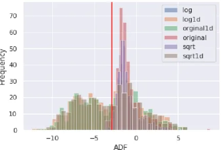
The ADF tests the null hypothesis of the presence of the unit root against an alternative hypothesis of series being stationary, where the ADF t-statistic is the result of the least square estimates for the regression in Equation 8.
ADFt= ˆ
φ−1
SE(φ) (9)
When the ADF test is applied to the original non-differenced series, I fail to reject the null-hypothesis, implying that series are non-stationaryI(0)in most of the cases and need to be differenced. Non-stationarity is quite common for financial series. The original series are first differenced, and the ADF test is applied to theI(1)series, I reject the null hypothesis for the majority of the series for 2002-2007 samples and conclude that the first differencing is sufficient to make the series stationary. In general, the mean-reverting aspect (no unit root) of the long term implied volatility has been empirically observed due to the long-memory of the volatility series. The unit root cannot however be entirely rejected because, in the short term, the unit root is often observed, which is attributed to the sudden spikes in short term volatility because of the crash-like behavior of the underlying asset or other extreme events. In fact, the impact of heterogeneity of these volatility returns is addressed by Corsi (2008). The findings that non-differenced IV series follow a non-stationary process are somewhat inconsistent with the earlier research. Although sampling methodology and sampling window or even the IV instrument can
Figure 3: ADF Test for 2002-2007.
also be attributed to differences in ADF results, as previous researchers indicate, these differences are attributed to sampling period or the methodology of constructing the volatility series (Gospodinov, Gavala, and Jiang, 2006). As the result of these findings, I continue treating the volatility series asI(1)process
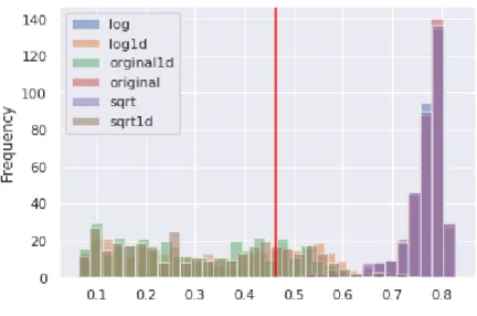
As a complement to the ADF test, I conduct the KPSS test (Kwiatkowski
et al., 1992) to test whether series are level stationery. KPSS test decomposes IV seriesVt
into deterministic, random walk and stationary error term:
yt=Tt+zt+ηt (10)
whereTtis a deterministic linear trend,ztis a random walk with the properties
like Equation 8 andη ∼N(0, σ2)is the stationary error. The partial sum of OLS residuals
Stfrom Equation 10 is constructed to obtain the KPSS test statistic:
KP SS =n−2 n X t=1 S2 t ˆ σ2 (11)
Figure 4: KPSS Test for 2002-2007.
the test is that the data is level stationary, and the alternative is that the data is not level stationary. Similar to the ADF test, when the original series are first differenced, I fail to reject the null hypothesis for the majority of the series, concluding that the series are level stationary for the 2002-2007 sample.
Although it’s confirmed that no unit root is present in the majority of first differenced series, in some cases, the unit root was still present. To test whether the unit root is present cross-sectionally across the panel, I utilize Madwu fisher type test:
M ADW U =P =−2 N
X
t=1
lnpi (12)
wherepi is the p-value from the unit-root root test, that results in aχ2 distributionP.
Some advantages of the test are especially noteworthy in case of the IV panel data: 1) dimension ofN (contract series) can be finite or infinite, 2) each group can have it’s own set of stochastic or deterministic components, 3) unbalanced series may be present 4) unit root rule is not strictly enforced and would allow some groups to have unit root while others have no unit root. The null hypothesis matches the ADF null hypothesis, that unit root is present.
confirm that that individual intercepts are stationary. Because the test statistic is a
chi-squared distribution, I can conclude that although some series tend to exhibit unit-root, these series don’t significantly impact the overall stationarity of the panel, yielding critical values 8462.8 and 9436.2 respectively.
Now that I’ve established that the panel exhibits stationarity when first differenced. I am also interested in exploring a presence of any spurious correlation between groups, i.e if the linear combination of these series is stationary or not. In other words, with the help of the Johansen (1991) procedure, one can observe the existence of any common long-term equilibriums between the groups. This step is essential for the model selection, because if the series do not exhibit long-run relationships, then the usage of the long-term error correction models is not appropriate. I utilize the urca5 package in R to construct a Johansen test. The null hypothesis for the test isr= 0that no cointegration is present and alternative hypothesis is based on the number of cointegration equations. Based on the the critical values of the trace statistic in Table 2, I find strong evidence to reject the null hypothesis of no cointegration relations, and conclude that rank of the matrix is greater than 19, which implies that a combination of all series (moneyness groups) is needed to make the series stationary, so there exists a large number of cointegration relations.
Table 2: Johansen test trace statistic critical values. Relations Critical Value
r≤ 19 138.466 r ≤18 1622.217 r ≤17 3722.018 r≤16 5904.430 r ≤15 8191.562 r ≤14 10493.895 r ≤13 12835.898 r ≤12 15191.440 r ≤11 17551.433 r ≤10 19918.851 r ≤ 9 22286.508 r ≤ 8 24656.662 r ≤ 7 27028.054 r ≤ 6 29408.080 r ≤ 5 31795.009 r ≤ 4 34190.643 r ≤ 3 36605.766 r ≤ 2 39054.031 r ≤ 1 41648.846 r ≤ 0 47320.253
3.6 FORECASTING MODELS
The primary goal is to propose a forecasting methodology that as observed from the statistical tests incorporates: 1) series autocorrelation behavior 2) is able to
non-paramterically estimate the cointegrated behavior of the panel 3) accounts for long term error correction (or long memory of the series). The model evaluation process is based onyt+1...yt+30forecasting window results where the residual erroret=yt−yˆtis
minimized, and residuals of each model are diagnosed and checked for robustness by conducting several statistical tests and side-by-side comparisons of the predicted IVS. I summarize the findings in Chapter 5.
3.6.1 LONG-SHORT TERM MEMORY MODEL
Long Short Term Memory neural network (Hochreiter and Schmidhuber, 1997) is a type of recurrent neural network (RNN) that is often used for sequence learning. The network contains recurrent loops that help model retain the past information and carry it forward throughout time. Unlike a simple MLP where the layers and neurons are fully connected to each consecutive layer, and the weight and biases matrices of each layer are propagated unidirectionally forward, the RNN extension reuses the same set of weights that are shared across time. Sharing weights is not only beneficial for retaining the long memory of the input sequence but also an optimization step that makes RNN’s use less
computational resources than MLP’s. Given an input sequence:x= (xt1, xt2, ..., xtn)the
one layer hidden state at timet,ht=f(ht−1, xt)can be written as a function of the
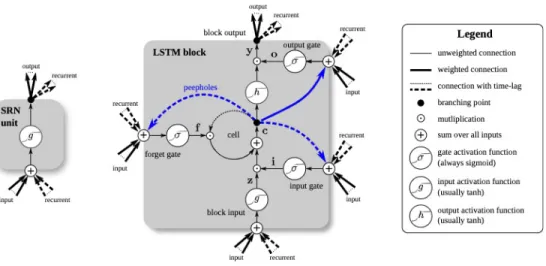
previous time stepht−1, which serves as a memory. However, this introduces a problem where the gradients can vanish or explode over time. During the backpropagation, the network accumulates the error gradients recurrently, which could cause large updates to the weights, making a cell output an infinitely large or small gradient. Hochreiter and Schmidhuber (1997) addressed this problem in their paper by expanding an RNN cell to include the forget and output gates, as shown in Figure 5. Forget gate and output gates are
Figure 5: Simple RNN cell and LSTM memeory cell as presented in Greff et al. (2017).
the most critical component of the LSTM (Greff et al., 2017). When the sequence passes through an input gate, the hidden state from the previous timesteps and the current timestep pass through an activation function (hyperbolic tangent) and then a forget gate (sigmoid), which dictates whether the new hidden state should be updated and carried forward to the next time step. The simple RNN cell, on the other hand, contains no gates, so the information flow is purely controlled by the activation function.
The model is implemented in Google’s deep learning framework Keras6 and the flow for the models is generated in Tensorboard7 and visualised in Figure 6. The input passes through a LSTM cell, and the hidden state of the cell at each of 30-time steps passes through a dropout layer, which randomly drops the connections for the output of the hidden state lstm 15 to reduce the possibility of over-fitting. A second LSTM layer is stacked to extract the time distributed hidden state from the first LSTM layer, and finally output a fixed 30-day (-1,30,80) vector as an output of the fully connected dense 8 layer.
6https://keras.io/
Figure 6: LSTM and ConvLSTM model flowcharts.
3.6.2 CONVOLUTIONAL LONG-SHORT TERM MEMORY MODEL
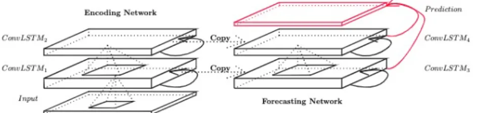
The main disadvantage of the simple fully connected LSTM (FC-LSTM) for IVS forecasting is that the inputs are flattened before being passed to the hidden state, so the essential spatiotemporal relations of the IVS are lost. This is addressed by Shi
et al. (2015), who proposed an extension to the FC-LSTM, which adds additional filter dimensions to the cells, hidden states and output gates. The proposed model determines the future state of the fixed-size cell in the grid by the inputs at current time-step, and the previous states of it’s neighboring cells, as visualized in Figure 7.
As shown by Shi et al. (2015) the ConvLSTM is shown to consistently outperform the fully connected LSTM on multiple spatiotemporal datasets, on various configurations.
Figure 7: Forecasting ConvLSTM as presented in Shi et al. (2015).
The researchers found that larger kernel size significantly helps the receptive fields in capturing the spatiotemporal correlations and spatiotemporal motion patters, with a smaller number of parameters required. The convolutional filter on its own adds a layer of non-linearity, which is quite relevant for modeling the IVS. During the convolutional operation, the fixed-sizedN ×M grid, known as a filter (kernel), slides over the shape of the IVS and continuously adjusts its weights. Orosi (2012) describes that the majority of the practical methodologies for modeling and interpolating the IVS rely on non-linear methods such as fitting the quadratic function, cubic spline, or a low-order polynomial, so the mechanics of the ConvLSTM seem to align well with the mechanics of the IVS.
The model is also implemented in Google’s deep learning framework Keras, and the flow for the models is generated in Tensorboard and visualized in Figure 6. While a FC-LSTM accepts the 3D vector shaped as (batch, timesteps, features), the ConvLSTM accepts the 5D input vector of (batch, timesteps, rows, columns, features), where rows and columns represent the grid as shown in Figure 7.
I also add a pooling layer to reduce the dimensionality of the input. An additional benefit of using a pooling layer is addressing the mean-reverting property of the IV. The average pooling layer of the ConvLSTM extracts average past states of the neighboring features, which helps maintain long term dynamics of the IV. Similar to the LSTM architecture, I stack a second ConvLSTM layer, to capture a more detailed representation of the first ConvLSTM layer. Following a second ConvLSTM layer, the outputs are flattened and fully connected to a simple, fully connected (dense) layer, which is shaped
as a fixed 30 timestep vector of size (1,30,80), to produce a fixed 30-day forecast for all 20 log-moneyness groups and 4 months (March, June, September, December).
3.6.3 VECTOR AUTOREGRESSION MODEL
From the stationarity test, I found that series are stationary when first differencedI(1), and due to the multivariate regression requirement I use Vector Autoregression (VAR) model:
ˆ
yt=A1yt+. . .+Akyt−p+ut (13)
whereyˆtis aK×1vector of either forecastyt+ior lagged observationyt, yt−1, ..., yt−p,
A1, ..., AkareK coefficient matrices andutrepresents k-vector of error terms. The lag
term for the model was selected based on the PACF and turned out to be significant only at lag 1. VAR model gives a good baseline model, but because significant cointegrated relationshipsr >0are evident between contract log-moneyness groups and expiration months, the error correction term (EC) can be added to the VAR model to account for the long-term relationships (stochastic trend) and still be able to capture the short term dynamics, to improve the forecast.
3.6.4 VECTOR ERROR CORRECTION MODEL
As observed in Johansen procedure, the volatility series experience long-run cointegrated behavior, so the Vector Error Correction Model (VECM) is a restricted VAR model, where the large swings in the short term can be restricted and converged to their cointegrated (long-term) relation. So Equation 13 can be rewritten to include the cointegrated transformation: ∆ˆyt = Πyt−1 + p−1 X i=1 Γi∆yt−1+ut (14)
whereΠ =I−Π1+...+ Πis a long-run relationshipk×kmatrix andΓ = Γ1+...+ Γi
is a short run relationship.
4 ALGORITHMS AND OPTIMIZATIONS
I follow a traditional time series forecasting and backtesting methodology using a train-test split that preserves temporal ordering. This is done for the time-series and the neural networks to have similar and comparable results:
Algorithm 2: VAR and VEC training and validation algorithm. train ←− Select all from prepared dataset where day <2007-08-17 test ←− Select all from prepared dataset where day > 2007-08-17
if VAR(1) then
∆ train = traint - traint−1
model fit Xt−1
model predict Xt+90
predict inverse = ∆ train += model predict
return MAPE, RMSE ←−test - predict inverse
end if
if VEC(1,1) then
model fit Xt−1
model predict Xt+90
return MAPE, RMSE ←−test - predict
end if
Algorithm 2 is modified to interface with R to produce the VAR and VEC models using tsDyn8 package in R.
In addition to the algorithm implementation with the deep learning framework Keras, a number of modifications to the LSTM and ConvLSTM Algorithm 3 were done: The data was transformed into a supervised learning problem where the data is
reorganized into 2 groups: an input group: X =Xt−1, Xt−2, ..., Xt−30and the target group:Y =Xt, Xt+1, ..., Xt+30, to match the fixed 30 day prediction window of the VAR and VEC models. The implemented design utilizes a sliding window approach to help maintain a universal model that can pick up from anywhere in the sequence yet still
Algorithm 3: LSTM and ConvLSTM training and validation algorithm. train ←− Select all from prepared dataset where day <2007-08-17 test ←− Select all from prepared dataset where day > 2007-08-17
Function SUPERVISED(data, history days, prediction days):
x = data.shift t−history days; y = data.shift t+prediction days
return [x, y]
Function SCALE(data): return data.scale(-1,1)
Function INVERSE SCALE(data): return prediction inverse scale
if LSTM then
model ←−reshape(n, 30, 80) ←− SCALE(.) ←− SUPERVISED(train, 30, 30) model train for 1000 epochs
end if
if ConvLSTM then
model ←− reshape(n, 30, 20 , 4, 1) ←− SCALE(.) ←− SUPERVISED(train, 30 , 30)
model train for 1000 epochs
end if
for i in range 3 do
model predict Xt+30
INVERSE SCALE(prediction)
end for
produce meaningful forecasts. By default, the LSTM in Keras is stateless and treats each batch sequence independently from the previous batch, and resets its internal memory state for each batch; this is done so that the back-propagation algorithm could run between batches and update the weights. Because it’s important to carry forward volatility
relationships for the lengthy periods of time as discussed in Section 3.5, each batch contains a fixed 30-day history window and produced a fixed output window, which classifies both LSTM and ConvLSTM models, as many-to-many models. This allows us to carry forward the weights from the past time-windows effectively, learning a long-term dependency of the volatility series. I begin by first scaling the features into a range of -1 and -1 due to the hyperbolic tangent activation function in the LSTM and ConvLSTM hidden layers, before training.
The model is configured to save weights at each epoch and finally retain the best weights for the models based on the lowest in-sample forecasting mean-squared-error (MSE). For both models, I set the training period for 1000 epochs and add an early
stopping callback to stop the training once no improvements in the MSE were made for 50 epochs. The LSTM was trained for 1000 epochs, which took approximately 1 hour and 20 minutes on Google’s Research Colab9 GPU environment.
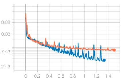
The ConvLSTM was trained for 851 epochs, triggering an early stop after approximately 1 hour and 30 minutes. The training process is visualized in the Figure 8. A similar reduction in MSE for both LSTM and ConvLSTM is observed; however, the LSTM has a larger training variance when compared to the ConvLSTM. This is an inherent problem when constructing data-driven supervised learning models, often referred to as bias-variance tradeoff. High bias in the context of neural network-based supervised learning architectures would mean that the model is underfitting the data, so adding more data, or hyperparameter optimization such as increasing the number of neurons, network depth or learning rate, might assist in capturing more complex feature
Figure 8: LSTM (blue) vs ConvLSTM (orange) training process with minimizing scaled IV MSE.
representation. High variance, on the other hand, means that the model is overfitting the data and captures random noise. For the purpose of constructing the IVS, both low variance and low bias are important, but because of this tradeoff, one must tune the hyperparameters to achieve the optimal balance between bias and variance. The LSTM produces overall lower training error, however experiences higher variance. ConvLSTM has a slightly higher (MSE) training error but overall lower variance.
Both models output a 30-day IVS prediction vector. For the LSTM and
ConvLSTM, the transformation is a three-step process. Original training values are first scaled to a range of -1 to 1 due to the hyperbolic transfer function in the hidden layer. Appropriate scaling has been shown to significantly improve the out-of-sample neural network performance for implied volatility forecasting (Liu, Oosterlee, and Bohte, 2019); output of the recurrent hidden layer is flattened and connected into a 1d fully connected output layer shaped1×20×4×30; an output vector is inverse scaled to the original BS-IV volatility level, as discussed in Section 4. The output vector is a 30-day prediction window for the March, June, September, December month contracts for each of the 20 log-moneyness categories, 10 for the OTM puts, and 10 for the OTM calls.
5 RESULTS AND DISCUSSION
In this section, I discuss the results of the machine learning models and finally compare the forecasting accuracy of these models to the benchmark VAR and VEC model. The comparison is made out of two subtopics to answer two questions: 1) Which of the models performs the best for the 1-day, 30-day, and 90-day windowed forecast. To support the findings, I conduct the (Diebold and Mariano, 1995) (DM) test for the equal predictive accuracy of the models 2) Which of the models can correctly model and predict the IVS dynamics. I conduct a Welch’s t-test to test whether the distribution of the
predictions is significantly different and test whether the models can capture the skew and the term structure of the IVS. 4 models are compared side-by-side, and the evaluation is based on the 90 trading-day hold out period from 2007-08-17 to 2007-12-31 over a 1-day, 30-day and 90-day prediction windows. In this section, I present findings that convolution operation in the LSTM memory cell, significantly improves modeling and forecasting future implied volatility and outperforms traditional time-series approaches for long-horizon predictions.
5.1 MODEL EVALUATION CRITERIA
In Section 3.1, I discussed the interpolation technique, to fill the missing values after pivoting the option chain. Before scoring the models, the predictions are inverted back to the original BS-IV volatility level, and scoring is based on the original BS-IV. For the VAR Model, the data was initially first differenced to achieve stationarity, so the predicted observations are added back to the non-differenced values, to recreate the original
continuous volatility series. For the VEC model, the output is an IV volatility of an appropriate scale, so the inverse difference is not necessary10. To fairly compare the models, all 4 models are trained on the same training set of 1370 days. One of the
10Differencing in the VEC model is done internally thought an implementation in the tsDyn library in R, through the integration and co-integration factor parameter
differences in the supervised, sliding window approach for the LSTM and ConvLSTM, when compared to the VAR and VEC models, is that the forecast is a fixed size 30-day vector. The LSTM and ConvLSTM are not retrained for the 90 trading-day out-of-sample predictions. Instead, the 30-day historical window is passed as an input to the model, to get the next fixed 30-day forecast window. This is done because the LSTM learns to generalize the sequences and can predict sequences based on the weights learned from the long series. To make the comparison between the neural networks and time-series models fair, The VAR and VEC models are fit on a train set, and the same set of coefficients is reused for predicting 1-day, 30-day, and 90-day windows. As the evaluation criteria I choose: RM SE = v u u t 1 N N X i=1 (σactual−σf orecast)2
where the RMSE metric is expressed in the actual BS IV volatility level, and:
M AP E = 100% n n X t=1 σactual−σf orecast σactual
MAPE is expressed as a real percentage point difference between the actual and the predicted BS-IV. I compare the performance of the models based on the RMSE, MAPE for the entire prediction vector. These loss metrics were chosen to be consistent with previous machine learning research in the area of IV modeling and forecasting, which tends to use a combination of MSE, RMSE, or MAPE (Gospodinov, Gavala, and Jiang, 2006; Xiong, Nichols, and Shen, 2016; Culkin and Das, 2017; Luong and Dokuchaev, 2018; Liu, Oosterlee, and Bohte, 2019).
Lastly, I conduct the Welch’s t-test to test whether the distribution of the
predictions is significantly different across groups, and the DM test for significance of the forecasts at various time horizons.
Table 3: Mean in-sample performance, mean out-of-sample performance and Savitzky-Golay filter smoothed prediction performance on the out-of-sample set.
Model In Sample Out-of-Sample Out-of-Sample(filter smoothed)
RMSE MAPE RMSE MAPE RMSE MAPE
VAR 0.194 102.89 0.041 19.28 0.04 18.87 VEC 0.193 102.88 0.041 19.13 0.04 18.75 LSTM 0.020 3.49 0.068 20.07 0.06 18.60 ConvLSTM 0.045 4.29 0.030 12.28 0.03 11.35
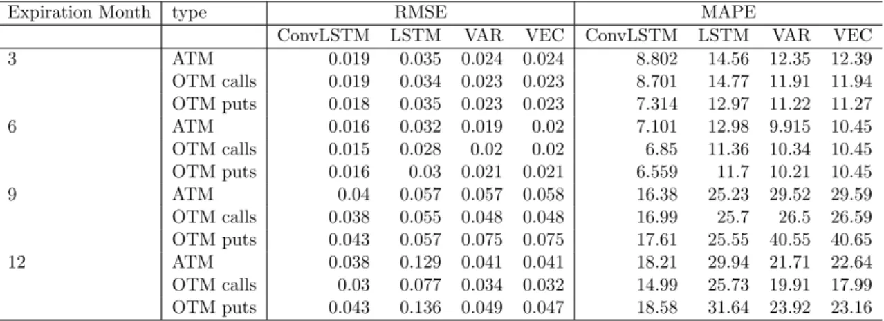
Table 4: Mean out-of-sample RMSE and MAPE grouped by expiration month and contract type.
OTM call buckets are X > 0.001, OTM puts are X < −0.004 and ATM buckets are X >−0.004;X <0.001, where X =ln(K/S) group.
Expiration Month type RMSE MAPE
ConvLSTM LSTM VAR VEC ConvLSTM LSTM VAR VEC 3 ATM 0.019 0.035 0.024 0.024 8.802 14.56 12.35 12.39 OTM calls 0.019 0.034 0.023 0.023 8.701 14.77 11.91 11.94 OTM puts 0.018 0.035 0.023 0.023 7.314 12.97 11.22 11.27 6 ATM 0.016 0.032 0.019 0.02 7.101 12.98 9.915 10.45 OTM calls 0.015 0.028 0.02 0.02 6.85 11.36 10.34 10.45 OTM puts 0.016 0.03 0.021 0.021 6.559 11.7 10.21 10.45 9 ATM 0.04 0.057 0.057 0.058 16.38 25.23 29.52 29.59 OTM calls 0.038 0.055 0.048 0.048 16.99 25.7 26.5 26.59 OTM puts 0.043 0.057 0.075 0.075 17.61 25.55 40.55 40.65 12 ATM 0.038 0.129 0.041 0.041 18.21 29.94 21.71 22.64 OTM calls 0.03 0.077 0.034 0.032 14.99 25.73 19.91 17.99 OTM puts 0.043 0.136 0.049 0.047 18.58 31.64 23.92 23.16 5.2 RESULTS
In Table 3, I summarize the mean in-sample, out-of-sample, and out-of-sample errors with the Savitzky-Golay filter applied. Much lower in-sample RMSE and MAPE for the
ConvLSTM and LSTM are observed, which could be attributed to an ability of the neural networks to accurately approximate the BS-IV (Liu, Oosterlee, and Bohte, 2019; Culkin and Das, 2017). Liu, Oosterlee, and Bohte (2019) used neural network for estimating three IV equations (BS, Heston, Brent’s) and found that neural network is highly efficient at approximating option prices and IVs, and because of the ability to “batch” process the contracts, it can lead to significant performance gains for on-line predictions. Culkin and
Table 5: Average out-of-sample forecast, for 1-day, 30-day, 60-day, and 90-day hori-zons.
Model horizon RMSE MAPE VAR h=1 0.020 6.06 h=30 0.042 20.46 h=60 0.044 22.10 h=90 0.041 19.28 VEC h=1 0.019 5.95 h=30 0.042 20.41 h=60 0.044 21.97 h=90 0.041 19.13 LSTM h=1 0.077 38.32 h=30 0.033 11.96 h=60 0.041 17.73 h=90 0.068 20.07 ConvLSTM h=1 0.025 7.80 h=30 0.030 11.14 h=60 0.027 11.18 h=90 0.030 12.28
Das (2017) found that ANN’s can learn to price options with the BS equation and produce very low error rates.
The out of sample forecasts are divided into multiple time horizons, which are summarized in Table 5. The horizon represents a daily mean IV across all log-moneyness and maturity groups. It’s observed that LSTM and ConvLSTM have overall higher RMSE and MAPE for a 1-day prediction horizon when compared to VAR and VEC models, and for the LSTM the RMSE and MAPE are reduced for a 30-day forecasting horizon, the errors become substantially larger for a longer forecast. For the ConvLSTM, the error increases slightly from a 1-day forecast but remains near-constant for multiple forecasting horizons. This behavior confirms observations of Shi et al. (2015) that were described for a number of spatiotemporal datasets, that 1) the ConvLSTM is better at handling
spatiotemporal relationships than a regular fully connected LSTM and 2) larger kernel sizes allow for the capture of the spatiotemporal motion patterns. By using an additional average pooling layer between two ConvLSTM layers, it also allows us to capture the
mean-reverting nature of the implied volatility over a long-term horizon allows and show that historical spatial relationships between the maturities play an important role in the forecasting of the IVS.
Figure 9: Average out-of-sample predicted IV.
Average predictions against true values are visualized in Figure 9. It is observed that all 4 models seemingly predict the average IV pattern but overestimate the IV jumps and magnitude of these jumps in the longer-term. Time-series models converge to a mean value following 10 timesteps, and the output of the VAR and VEC model is the average IVS of previous timesteps. The VEC model performs better than the VAR model due to the cointegrated relationships between moneyness groups and maturities that are
significantly impacting the performance of the model. Because machine learning models use a different architecture, the output IVS can be produced given the input IVS. The LSTM produces a smoother forecast but experiences a period of instability from 2007-11-1 to 2007-12-14, as seen in Figure 9. This behavior can be observed for other
models as well, but machine learning models show better overall forecasting performance. ConvLSTM produces a lower degree of under-estimation for long-term contracts.
ConvLSTM produces the closest prediction to the actual IV, which implies that
meaningful information is extracted during convolution operation over the volatility skew and the term structure, which is subsequently captured in the average pooling layer. The significance test for the forecasts at multiple time horizons and the side-by-side
comparison between the models is summarized in Table 6.
To mitigate the effect of the forecast instability, I apply the Savitzky-Golay smoothing filter based on the 4th degree polynomial for each of the predicted 30-day windows and plot it against the true IV in Figure 10. Similar to that of the unsmoothed forecast, VAR and VEC models overestimate the IV level, but seemingly capture the future dynamics of IVS. For LSTM and ConvLSTM smoothing the forecast with the Savitzky-Golay filter helped reduce some of the output noise, that was observed in the raw forecast. By applying the Savitzky-Golay smoothing filter, I saw a reduction in RMSE and MAPE cross-sectionally for all models, and summarize the results in Table 3.
I construct a mean predicted IVS for the 90-day holdout period and compare it to the mean actual IVS for the same period to investigate whether the future general
dynamics of IVS are captured by the VAR, VECM, LSTM and ConvLSTM models. Figure 11e shows mean actual IVS is based on the same time-frame of 2007-08-17 to 2007-12-31 of the holdout window. The near term contracts observe higher IV levels than longer-term contracts. In addition, the volatility skew is also present in Figure 11e. As discussed in Section 3.4, the IVS is constructed by arranging 20 log-moneyness groups, where values<0, represent OTM puts, and values>0 represent OTM calls. So to properly capture the dynamics based on the holdout window, the models need to show overall presence of the IV term structure, which in the case of the holdout window is expressed through a higher IV for the September (Month 9) and December (Month 12) contracts. As a second criterion, the models also need to capture the skew properly. Figure
(a) VAR average predicted IVS. (b) VEC average predicted IVS
(c) LSTM average predicted IVS (d) ConvLSTM average predicted IVS
(e) Actual average IVS