J. David Cummins* Gregory P. Nini. June 29, 2001

OPTIMAL CAPITAL UTILIZATION BY FINANCIAL FIRMS: EVIDENCE FROM THE PROPERTY-LIABILITY INSURANCE INDUSTRY

By

J. David Cummins* Gregory P. Nini

June 29, 2001

J. David Cummins* Gregory P. Nini

The Wharton School The Wharton School

3641 Locust Walk 3641 Locust Walk

Philadelphia, PA 19104 Philadelphia, PA 19104

Phone: 215-898-5644 Phone: 215-898-5644

Fax: 215-898-0310 Fax: 215-898-0310

Email: [email protected] Email: [email protected] *Please address correspondence, page proofs, etc. to David Cummins.

Abstract

Capitalization levels in the property-liability insurance industry have increased dramatically in recent years – the capital-to-assets ratio rose from 25 percent in 1989 to 35 percent by 1999. This paper investigates the use of capital by insurers to provide evidence on whether the capital increase represents a legitimate response to changing market conditions or a true inefficiency that leads to performance penalties for insurers. We estimate “best practice” technical, cost, and revenue frontiers for a sample of insurers over the period 1993-1998, using data envelopment analysis, a non-parametric technique. The results indicate that most insurers significantly over-utilized equity capital during the sample period. Regression analysis provides evidence that capital over-utilization primarily represents an inefficiency for which insurers incur significant revenue penalties.

1. Introduction

Insurers hold equity capital to provide assurance to policyholders that claims will be paid if losses are higher than expected or if investment returns fall short of expectations. The objective is to attain an optimal level of insolvency risk that balances the marginal benefits and costs of holding equity capital. There are marginal benefits from holding capital because safer insurers command higher prices and because insurers risk losing customers if insolvency risk is perceived as excessive (Sommer 1996, Cummins and Danzon 1997). However, holding equity capital in an insurance company is costly due to regulatory costs, agency costs from unresolved manager and owner-policyholder conflicts, the costs of adverse selection and moral hazard in insurance underwriting and claims settlement, corporate income taxation (Cummins and Grace 1994), and other market frictions. Hence, insurers do not hold sufficient capital to eliminate insolvency risk; rather, insurers maintain market-driven ''safe'' or ''adequate'' levels of capital (Cummins, Grace, and Phillips 1999).1

A puzzle has developed in the property-liability insurance industry as capitalization has risen to unprecedented levels in recent years. The ratio of premiums written to surplus, the industry's standard leverage index, traditionally fluctuated around two. Beginning in the mid-1980s, however, the ratio began a precipitous decline and dipped below one at the end of 1999. Likewise, the equity capital-to-assets ratio, traditionally around 25 percent, increased to 35 percent by 1999. These developments raise questions about whether the industry is over-capitalized or whether structural changes in the insurance or capital markets have altered the optimal degree of capitalization.

The objective of this paper is to analyze capitalization in the property-liability industry to provide new evidence on whether insurers are over-utilizing equity capital. We employ a frontier efficiency approach to analyze capital utilization of property-liability insurers over the period 1993-1998. Using data envelopment analysis (DEA), a non-parametric technique, we estimate ''best

1 _{Regulation, including the National Association of Insurance Commissioners (NAIC) risk-based capital system,}

specifies minimum levels of capital for insurers. However, the vast majority of insurers maintain significantly higher capital than required by risk-based capital rules (see Cummins, Grace, and Phillips 1999).

practice'' technical, cost, and revenue frontiers and measure the efficiency of each firm in the sample relative to the frontiers, producing estimates of technical, allocative, cost, and revenue efficiency.

A key concept that we use in analyzing insurer capital utilization is that of cost efficiency, which measures the firm's success in minimizing costs. Cost efficiency is defined as the ratio of the costs that would be incurred by a fully efficient firm producing the firm's outputs to the costs actually incurred by the firm. Thus, fully efficient firms have cost efficiencies of one, and inefficient firms have cost efficiency between zero and one. Cost efficiency can be decomposed into technical efficiency and allocative efficiency. Technical efficiency measures the firm's success in using state-of-the-art technology, i.e., in operating on the production frontier. Allocative efficiency measures the firm's success in choosing the cost minimizing combination of inputs, conditional on output quantities and input prices. To be fully cost efficient, a firm must operate with full technical and allocative efficiency. We also estimate revenue efficiency, which measures the firm's success in maximizing revenues. Revenue efficiency is defined as the firm's actual revenues divided by the revenues of a fully efficient firm that utilizes the same quantity of inputs. As with cost efficiency, technical, allocative, and revenue efficiency equal one for fully efficient firms and are between zero and one for inefficient firms. Lower efficiency scores indicate more inefficient firms.

The concept of allocative efficiency provides a natural way to analyze whether insurers are under- or over-utilizing capital. Allocative efficiency measures the extent to which a firm chooses the correct quantities of inputs in order to produce their outputs. Further, the estimation procedure generates estimates of the optimal input quantities for each firm in the sample. By comparing the actual capital for a given firm with its optimal capital, we can determine whether the firm is under or over-utilizing capital relative to the capital that would be used by a fully efficient firm with the same quantity of outputs.

There are two possible reasons why firms may be measured as under- or over-utilizing capital

in our DEA analysis. The first possibility is that measured sub-optimal capital utilization represents a rational response to market factors or firm characteristics that legitimately require differential capital utilization. If this explanation is correct, a firm's performance should not be adversely affected by differences between its actual capital and its measured optimal capital. The second possible explanation is that measured under- or over-utilization of capital represents a true inefficiency that degrades firm performance. To provide information on which explanation is correct, we utilize revenue efficiency and book-value return on equity (ROE) to measure firm performance and estimate the impact of capital utilization on these performance measures. We regress revenue efficiency scores and book-value ROE against a set of explanatory variables, including the ratio of the firms' actual less optimal capital to assets. This ratio, which we call the sub-optimal capital-to-assets ratio, represents the amount of capital under- or over-utilization relative to assets. A larger value for this ratio indicates excessive use of capital relative to our measured level of optimal capital. If measured sub-optimal capital utilization represents inefficiency, then we expect the sub-optimal capital to assets ratio to have adverse effects on firm performance, as explained in more detail below.2

In addition to measuring the effects of sub-optimal capital on firm performance, we specify and test several hypotheses regarding the characteristics of firms that are likely to be associated with capital utilization. We regress the ratio of the firm’s actual-to-optimal capital against a vector of explanatory variables representing the theoretical hypotheses. These tests enable us to control for differences among firms that may help to explain observed patterns of capital utilization in the industry.

By way of preview, we find that the run-up in equity capital of the past decade is primarily attributable to capital gains on investments. Further, we provide evidence that capital levels in the industry are ''sticky'' in the sense that insurers are reluctant to pay out capital accumulations as

2 _{We also perform similar regressions to test if the effect is symmetric for under and over-utilization of capital. By}

separating the sub-optimal capital-to-assets ratio into positive and negative components, we test whether any adverse effects of sub-optimal capital utilization differ depending upon whether the insurer is under- or over-capitalized.

dividends, preferring to maintain internal funds to cushion the loss or investment shocks. Finally, we find that insurers are substantially over-utilizing equity capital and that the over-utilization represents inefficiency that leads to significant revenue and cost of capital penalties for inefficient firms.

The remainder of the paper is organized as follows: Section 2 provides an empirical overview of capitalization trends in the property-liability insurance industry to provide background for the subsequent discussion. In section 3, we formulate hypotheses about insurer capital structure and specify the variables used to test the hypotheses. Section 4 discusses hypotheses and variables regarding revenue efficiency and ROE. Section 5 discusses our estimation methodology, and section 6 describes our sample and specifies the inputs and outputs used in the DEA analysis. The results are presented in section 7, and section 8 concludes.

2. CAPITALIZATION TRENDS IN PROPERTY-LIABILITY INSURANCE

Leverage ratios for the property-liability insurance industry for the period 1970-1999 are graphed in Figure 1. Two leverage ratios are shown - the ratio of net premiums written to equity capital (surplus) and the equity capital-to-assets ratio. The former is the traditional leverage ratio used in the industry, while the latter is used more commonly in the financial institutions literature. Both leverage ratios illustrate that equity capitalization in the industry has increased dramatically over the past fifteen years. The premiums-to-surplus ratio was near 2.0 in 1985 but then began an almost uninterrupted decline to less than 1.0 by 1999. The capital-to-assets ratio, which stood at 25 percent in 1985, increased to 37 percent by 1999.

The trends in the leverage ratios are primarily due to growth in insurer equity capital. During the ten-year period 1990-1999, equity capital growth averaged 10 percent per year (on a book basis), while premium growth was only about 3 percent per year. The divergent growth rates in capital and premiums are shown in Figure 2, which graphs the six-year moving averages in the growth rates for these two variables. Except for brief periods such as the mid-1980s, the growth rate in capital has far

exceeded the growth rate in premiums. During the 1990s, the capital growth in the industry tracks the bullish stock market (see further discussion below).

What can explain the dramatic changes in capital structure in this industry? There are several possibilities, most of which are explored in more depth below:

(1) The introduction of a risk-based capital (RBC) system by the National Association of Insurance Commissioners (NAIC) in 1994. The introduction of the RBC system was widely anticipated and may have led insurers to accumulate more capital to reduce the probability of incurring regulatory costs under the new system.

(2) The rise in importance of rating agencies. The insurance product market is known to react to ratings downgrades by firms such as the A.M. Best Company, Standard & Poor's, and Moody's. For example, in the commercial lines market, it is necessary for insurers to maintain at least an A rating in order to avoid losing customers to competitors. The rating agencies have played a more aggressive role with respect to insurers following the run-up in insurer insolvencies in the late 1980s and early 1990s. Thus, some insurers may have accumulated additional capital to protect their financial ratings.

(3) The growth in the market for alternative risk transfer products, which provide a substitute for conventional insurance. These include self-insurance programs, captive insurance companies, and securitized financial risk transfer instruments. These products have drained many of the more predictable risks out of insurance markets, increasing the overall volatility of insurer liability portfolios. Additionally, the rise of the alternative market has caused premium growth to stagnate, partially accounting for the gap between premium and equity growth.

(4) An increased awareness by insurers of their exposure to catastrophic property losses coupled with inadequate supply of reinsurance for such losses. Following hurricane Andrew in 1992 and the Northridge earthquake in 1994, insurers revised upward their estimates of potential losses due to catastrophes such as hurricanes and earthquakes. Simultaneously, it became apparent that

reinsurance for these large events was inadequate (Swiss Re 1997, Froot 1999). Thus, insurers with significant catastrophe exposure may have added capital to cushion catastrophic loss shocks. (5) The 1990s bull market in corporate equities, combined with insurer reluctance increase

stockholder dividends. There is both theoretical and empirical evidence that there is considerable ‘stickiness’ among insurers in adjusting dividends in response to increases in equity (Winter 1994, Gron 1994, Cummins and Danzon 1997). The stickiness is driven by informational asymmetries that make it difficult for insurers to raise capital after a loss or investment shock, inducing them to hold onto capital windfalls in anticipation of the next underwriting crisis. (6) Agency costs and other aspects of insurer organizational and market structure. These factors,

including the role played by mutual insurers, are discussed in more detail below.

Tracing the source of the industry's growth in equity capital may provide some initial answers to the capital structure puzzle. Table 1 breaks down the industry's growth in book equity into its sources and uses for the period 1989-1998. Section A of the table shows that total capital grew by $215.7 billion from 1989-1998, net of $78.8 billion in stockholder dividends and $29.4 billion in miscellaneous outflows. These capital disbursements are added back to the net change in capital to give the gross change in capital, and section B of the table shows the percentages of the gross change from each source of capital.

Capital gains provided the most important source of new capital during the ten-year period 1989-1998 and the four-year period 1995-1998, accounting for 51.7 percent during the former period and 57.0 percent during the latter. The second most important source of gross new capital is retained earnings (net underwriting income plus investment income), and the third most important source is new capital paid-in, from new equity offerings or contributions from parent firms. The uses of the gross changes in equity are shown in section C of the table. Insurers paid out as dividends about one-fourth of the total gross change in capital while retaining about two-thirds, with the remainder devoted to miscellaneous uses.

Table 1 provides some support for the capital stickiness hypothesis, i.e., that capital accumulates because insurers are concerned about the feasibility of raising new capital following the next major underwriting or investment shock. The last column in section A of the table shows the dividend payout rate over the period, i.e., the ratio of stockholder dividends paid to the total gross change in capital. The average payout rate is significantly lower in the second half of the sample period than during the first half, even though the second half of the sample period accounted for about 70 percent of the total change in gross capital. This is consistent with the view that insurers are reluctant to reduce capital during periods of capital growth by increasing the dividend payout rate.

3. Hypotheses: Capital Structure and Leverage

In this section, we discuss economic factors that influence insurer decisions about capitalization and formulate hypotheses about insurer capital structure based on financial theory. In addition to discussing the rationale for insurers to hold capital, we also formulate hypotheses about firm characteristics likely to be associated with under- and over-capitalization.

3.1 Financial Distress

The costs of financial distress are a common friction identified as influencing capital decisions. As insurers increase their capital relative to premiums or liabilities, the probability of insolvency declines, reducing the associated expected costs of financial distress. However, holding capital in an insurance company is costly because of various frictions and market imperfections, including agency costs, costs arising from adverse selection and moral hazard, regulatory costs, and corporate income taxation (Merton and Perold 1998). Agency costs for an insurer include the costs of unresolved owner-manager and policyholder-owner conflicts. For example, managers may take actions that are inconsistent with the maximization of firm value such as failure to invest in positive net present value projects whose risk may be a threat to managerial job security. Insurance markets are characterized by adverse selection and moral hazard, which lead to higher costs of capital to the extent that they cannot be fully controlled through contract design, underwriting, and the claims

settlement process. Finally, insurers incur significant regulatory costs and costs from corporate income taxation to the extent that these costs cannot be fully passed along to policyholders in premium rates charged for insurance (Cummins, Grace, and Phillips 1999, Cummins and Grace 1994). Because of these and other capital costs, insurers do not hold sufficient capital to reduce the probability of bankruptcy to negligible levels.

Financial distress occurs when an insurer has difficulty honoring commitments to policyholders and other creditors. The associated costs include the transactions costs of bankruptcy, the loss of talented employees, the loss of non-marketable and relationship-specific assets, reputation losses, and other losses to the insurer's franchise value. Further, insurance is priced as risky debt, and the prices an insurer's products command in the market are inversely related to the probability of bankruptcy (Sommer 1996, Cummins and Danzon 1997).

All else equal, as the expected costs of insolvency increase, the marginal benefit from holding equity capital increases, and the optimal leverage ratio (e.g., premiums-to-surplus or liabilities-to-surplus) decreases. For an insurance company, the probability of insolvency is related to an insurer's ability to diversify risk. As proxies for insolvency risk, we define three measures of liability risk and one measure of asset risk.

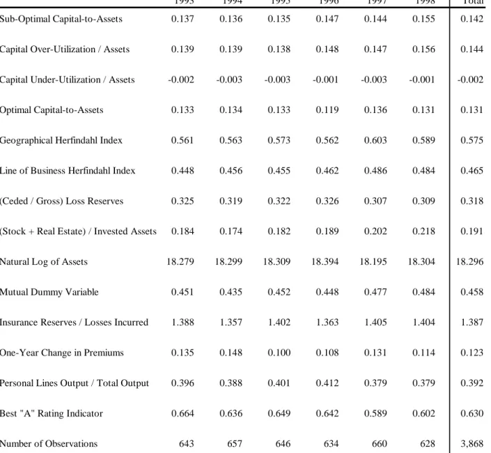
The first measure of liability risk is the insurer's diversification across geographical areas. Other things being equal, an insurer that is more geographically diversified is expected to have lower insolvency risk than insurers that are more concentrated geographically. To measure geographical diversification, we use a Herfindahl index of insurer premium writings by state. The second measure of liability risk is the insurer's Herfindahl index across lines of insurance based on premium volume.3 Insurers that are more diversified by line are expected to have lower insolvency risk than insurers concentrating on one or a few business lines. Lower Herfindahl indices imply higher diversification

3

The Herfindahl indices are, respectively, the sum of squares of the percentages of premiums written by state and the sum of squares of the percentages of premiums written by line.

and, consequently, the geographical and line of business Herfindahl indices are predicted to be positively related to the use of capital.

The third measure of liability risk focuses on the insurer's use of reinsurance. Because reinsurance represents diversification among insurance companies, firms that purchase more reinsurance are expected to have lower insolvency risk. Our measure of the intensity of an insurer's reinsurance activities is the ratio of ceded loss reserves to direct plus assumed loss reserves.4 We predict an inverse relationship between the reinsurance variable and the utilization of capital.

The measure of asset risk used in our analysis is the percentage of an insurer's assets invested in stocks and real estate, because these assets expose insurers to more volatility risk than their fixed income investments, which tend to be highly rated bonds and notes. We expect a positive relationship between the percentage of assets in stocks and real estate and the utilization of capital. These propositions are stated formally in the following hypotheses.

H1. The Herfindahl indices of premiums written by state and by line of business will be positively related to capital utilization.

H2. Firms with higher ratios of ceded loss reserves to direct plus assumed loss reserves will use less capital.

H3. Firms with higher percentages of assets invested in stocks and real estate will use more capital.

Part of the increase in capitalization levels in the insurance industry may be attributable to changes in the characteristics of insured risks. Buyers have substituted a variety of ''alternative risk transfer'' mechanisms for insurance, removing the more predictable risks and continuing to insure the more volatile risks such as commercial liability claims. If insurer liability portfolios have become increasingly volatile, this could provide an explanation of recent capitalization trends.5 Risk levels

4

Ceded reserves are the liabilities that an insurer transfers to reinsurers. Direct reserves represent the insurer's obligations in the primary insurance market, and assumed reserves reflect its obligations to other insurers as a reinsurer. Larger ratios of ceded loss reserves to direct plus assumed reserves indicate more use of reinsurance.

5

Changes in asset portfolio risk also could help to explain the changing capitalization levels in the industry. However, except for an increase in the proportion of assets held in corporate equities, primarily due to unrealized

also are expected to differ cross-sectionally among firms in the industry as a function of both underwriting and investment portfolio choices. To control differences in income volatility across insurers, we use the standard deviation of each insurer's book-value ROE computed over the three years preceding each analysis year. We expect this variable to be positively related to capitalization. H4. Higher risk, as measured by the standard deviation of ROE, will be associated with higher capital utilization.

It is well known from statistical and actuarial theory that the average loss in a pool of risks becomes more predictable as the number of risks in the pool increases. This means that the losses of larger insurers are more predictable than those of smaller firms so that large firms should require relatively lower capitalization to achieve a given level of insolvency risk. Although in principle smaller firms should be able to achieve similar results through reinsurance, in practice reinsurance is costly due to frictions such as moral hazard, adverse selection, and the need to provide a profit to the reinsurer. Following the recent insurance efficiency literature (Cummins and Weiss 2000), we use the natural log of firm assets to represent firm size and propose the following hypothesis:

H5. Capitalization will be inversely related to firm size. 3.2 Agency Costs

There are two primary sources of agency costs in the insurance industry: owner-manager conflicts and owner-policyholder conflicts. Conflicts between owners and managers arise because managers do not share fully in the residual claim held by owners and have an incentive to behave opportunistically. Conflicts between owners and policyholders arise because policyholders' claims to assets have legal priority over owners' claims. Owners have an incentive to exploit policyholder interests by changing the risk structure of the firm or taking actions that increase the value of equity, perhaps by decreasing the value of the policyholders' debt claim on the firm.

The owner-manager conflict is a classic example of moral hazard, since the non-contractible

increased importance of corporate equities by including the ratio of stocks and real estate to total assets as an independent variable in our empirical analysis.

effort of the manager directly affects the value of the claim held by the owner. Without possessing a 100 percent ownership stake, managers face a reduced marginal benefit from investing their effort into the firm, altering the incentives for the manager to exert the optimal effort. This creates a significant agency cost that can be reduced by increasing leverage. Holding constant the managers' level of ownership, reducing equity capital increases the managers' stake in the firm, helping to align the interests of owners and managers. Reducing equity also decreases the amount of free cash available for managers to pursue private interests, such as taking on projects that increase the size of the firm but do not maximize the value of equity. Finally, additional leverage increases the probability of bankruptcy (a particularly costly event for managers), making value-destroying pursuits more costly for managers. Mitigating the conflict between managers and owners thus constitutes a benefit from increased leverage.

When owners and policyholders are separate classes of investors, a conflict arises because owners have a claim to firm value only beyond the claims of policyholders. Due to limited liability, equity ownership is equivalent to a call option on the value of the firm, making risky investments attractive to owners. Since policyholders bear much of the consequences of failed investments, policyholders prefer less risky investments. When the opportunistic behavior of owners is anticipated, the effect is incorporated into the price of insurance, and owners bear much of the cost of the incentive conflict. This cost can be reduced by decreasing leverage, which mitigates the price effect by reducing insolvency risk. Further, increasing the amount of equity capital relative to premiums reduces the benefit to owners from substituting riskier investments, making asset substitution less attractive. Mitigating the conflict between policyholders and owners thus constitutes a benefit from decreased leverage.

Jensen and Meckling (1976) argue that the optimal capital structure is determined by trading off the benefits from increased leverage (mitigating the owner-manager conflict) with the benefits

from decreased leverage (mitigating the owner-policyholder conflict). When the owner-manager conflict is particularly severe, firms may appear under-capitalized to the extent that agency costs are not fully reflected in the cost of capital used in our efficiency analysis. When the owner-policyholder conflict is severe, firms may appear over-capitalized.

Because both stock and mutual insurers are present in the insurance industry, organizational form provides an excellent proxy for the degree of agency costs inherent in an insurance firm. Compared with stock companies, mutuals control the owner-policyholder conflict by merging these two roles. However, the owner-manager conflict is more severe in the mutual ownership form because the mechanisms available for owners to control managers are much more limited than in the stock ownership form. In a rational market, one would expect the benefits from removing the owner-policyholder conflict to exceed the costs of unresolved owner-manager conflicts in mutual insurance firms. Consequently, the elimination of the owner-policyholder conflict is likely to result in a reduced marginal benefit from holding capital in mutuals, suggesting that mutuals may be less capitalized than stocks, other things equal. Mutuals also may have less need for capital than stocks because they tend to invest in less complex or less risky projects requiring limited managerial discretion in pricing and underwriting (Lamm-Tennant and Starks 1993). On the other hand, mutuals may have a greater tendency than stocks to hoard capital during profitable periods because of their limited ability to access capital markets in the event of a shock to capital. In addition, to the extent that holding additional capital provides benefits to managers (e.g., from controlling larger investment portfolios), mutuals may hold capital in excess of optimal levels because of a misalignment of policyholder and manager interests. Because we do not have an unambiguous prediction about ownership form, we state the following hypothesis in null form:

H6. Mutuals will not utilize capital more or less intensively than stocks.

Due to the time lag between payment of premiums and payment of claims, insurance firm managers are in control of policyholder funds for a significant period of time. This time lag offers

managers the opportunity for engaging in activities that provide private benefits, possibly to the detriment of the firm and policyholders. As the policy length and claims tail increases, the problem worsens; and there is a benefit to removing excess funds from the firm and increasing the bankruptcy probability. Reducing capital and increasing leverage can accomplish this. An insurer's loss reserve and unearned premium reserve are liabilities for losses not yet paid and premiums received for which service has not yet been provided. The ratio of the sum of loss and unearned premium reserves to incurred losses is used as a proxy for time lag between policy issuance and the payment of claims, with higher ratios indicating longer tailed business. As this ratio increases, the marginal cost of capital increases and firms are predicted to choose lower capital levels. Thus, we hypothesize that: H7. The ratio of reserves to losses incurred will be inversely related to capital utilization.

3.3 Asymmetric Information and Growth Opportunities

If corporate managers possess superior information about the firm's assets in place and new investment opportunities than do owners, Myers and Majluf (1984) argue that these information asymmetries may cause managers to forego positive net present value projects. This results in a ''pecking order'' theory of financing where managers prefer financing through internal funds and debt rather than issuing new equity. As the degree of asymmetry between managers and investors increases, this under-investment problem worsens and raising equity capital becomes more costly.

The implications of the Myers-Majluf theory for our analysis depend upon the degree of the informational asymmetry problem in the insurance industry and the response to the problem by the firms in the industry. Because property-liability insurers invest primarily in marketable securities, there are minimal informational asymmetries from the asset side of the balance sheet, except perhaps with respect to the credit risk of receivables from agents and reinsurers. The principal informational asymmetry for property-liability insurers arises from uncertainty about the true value of reserves for the payment of unpaid losses, which averages about 65 percent of total liabilities, industry-wide. A substantial component of the loss reserve represents insurer estimates of the claims to be paid in the

future on long-tail policies such as commercial liability insurance. Insurers have significant actuarial and accounting flexibility in determining the stated loss reserve, and most of the information needed to evaluate the accuracy of reserve estimates is not available outside the insurer. Hence, there are significant information asymmetries between managers and investors with regard to the liabilities for long-tailed insurance policies, especially in the commercial lines.

Insurers may respond to the informational asymmetry problem by building up slack capital during profitable periods to provide internal funds to invest in attractive future projects. Alternatively, insurers with relatively high information asymmetries may become more highly leveraged, especially during unprofitable phases of the underwriting cycles, because they are at a net disadvantage in raising new equity relative to insurers whose liabilities are more transparent to investors. That is, if insurers with the greatest reserving uncertainty have equal ability to generate retained earnings as insurers with more transparent liabilities, the former group will likely become more highly leveraged over time because its costs of raising external capital are higher. Moreover, firms with higher reserve uncertainty may actually be less successful in generating retained earnings because long-tail lines of insurance tend to generate less income from underwriting than shorter-tail lines. Thus, such insurers may be disadvantaged in raising both internal and external capital, implying that information asymmetries between managers and owners are more likely to lead to higher leverage rather than additional slack capital in the insurance industry. Another implication of the Myers-Majluf theory is that for any given degree of informational asymmetry, firms with more growth opportunities are expected to hold additional capital to avoid the need for raising costly capital in the future. This discussion suggests the following hypotheses:

H8. Firms with higher information asymmetries between managers and owners will be more highly leveraged than firms with lower information asymmetries

.

H9. Firms with more growth opportunities will hold relatively more equity capital.

The standard deviation of ROE over time is used as a proxy for the degree of information asymmetries between managers and investors. Insurers with low earnings volatility are assumed to

possess assets and liabilities that change very little over time, making their future profitability easily conveyed from manager to investor. However, insurers with higher volatility have operations that are less predictable, and therefore have more severe information asymmetries than less risky insurers. Based on this rationale, the standard deviation of ROE is predicted to be inversely related to capitalization. Recall, however, that H4 predicts a positive relationship between ROE risk and capital, based on the financial distress costs argument. Thus, the sign of this variable will depend upon the extent to which it measures firm opacity versus the probability of financial distress. The ratio of reserves to losses incurred, discussed in connection with H7, also serves as a proxy for informational asymmetries, to the extent that lengthening the claims payment tail increases uncertainty about reserve accuracy. The reserves variable thus has a predicted negative sign under both H7 and H9.

To proxy for growth opportunities, we use the one-year percentage growth rate in premiums. As the measure of growth increases, it is hypothesized that insurers will be motivated to hold more capital to be able to take advantage of growth opportunities using internal rather than external funds. Thus, the premium growth rate is predicted to be positively related to capital utilization.

3.4 Product Market Interaction

Because the purpose of insurance is to diversify risk and indemnify policyholders for losses due to contingent events, the insurance market is sensitive to insurer insolvency risk, and safer insurers command higher prices. In addition, positive switching costs and private information possessed by the incumbent insurer can create a significant advantage to remaining with the same insurer (Kunreuther and Pauly 1986, D'Arcy and Doherty 1990). Due to economies of scale and the existence of insurance brokers, corporate insurance buyers face significantly lower switching costs than personal buyers, making relationships with corporate buyers more fragile than those with personal buyers. The commercial lines insurance market is considered a ''commodity market,'' where buyers choose insurers on the basis of price, from the set of insurers with adequate (often A or better)

financial ratings (i.e., the market is characterized by a tendency for ''flight to quality''). Moreover, commercial lines buyers and their brokers are more proficient than individual buyers in assessing insurer financial quality, suggesting the following hypothesis:

H10. Capitalization will be inversely related to the percentage of an insurer's revenues coming from personal lines of insurance.

To test H10, we include in the regressions the ratio of the insurer's personal lines premiums to total premiums. This variable is expected to be inversely related to capitalization. We predict a negative coefficient on the personal lines variable based on the flight to quality argument.

3.5 Regulation

In response to an increase in insurer insolvencies in the 1980s and early 1990s, the National Association of Insurance Commissioners (NAIC) instituted risk-based capital (RBC) requirements in 1994. Various regulatory actions are stipulated if the ratio of the insurer's actual capital to risk-based capital falls below a series of thresholds beginning at 200 percent (see Cummins, Grace, and Phillips 1999). The introduction of risk-based capital created a regulatory option that reduced the market value of insurers. Because the option value is inversely related to capitalization, the introduction of RBC is predicted to have increased capitalization levels in the industry. To control for differences in capitalization by year, we include year dummy variables in our regression equations. If capital levels were adjusted following the RBC introduction year (1994), the coefficients of the year dummy variables may be larger in the later years of the sample period. On the other hand, if insurers anticipated the introduction of RBC, any capital adjustments may have occurred prior to our sample period, and the year dummy variable coefficients will have no systematic pattern.

4. Hypotheses: Revenue Efficiency and Return on Equity

In addition to regressions to explain insurer capital structure, we also conduct regressions designed to detect relationships between capital structure and firm performance. We use two indicators of performance - revenue efficiency and book-value return on equity (ROE). In this section, we discuss hypotheses and expected signs for the firm performance regressions.

4.1 Revenue Efficiency

The primary purpose of the revenue efficiency analysis is to determine whether measured capital under- or over-utilization is a rational strategy that is rewarded by the market with additional revenues or a true inefficiency that leads to revenue penalties. The maintained hypothesis about the relationship between capitalization and revenue efficiency is that insurance buyers are sensitive to insolvency risk but that insurance market equilibrium occurs at a non-negligible probability of default. The primary reason is that holding equity capital in an insurance company is costly because of the various market, tax, and regulatory frictions discussed above. Thus, at some point, the marginal benefit of adding capital to reduce insolvency risk falls below the marginal cost of the added capital, producing an optimal capital-to-assets ratio that maximizes firm value.

Our analysis of cost efficiency enables us to estimate the optimal quantity of capital for each firm in the sample. Firms will be rewarded or penalized for measured sub-optimal capital utilization depending upon whether holding capital that deviates from the measured optimum represents a legitimate response to market forces or a true inefficiency. Sub-optimal capital-utilization does not represent a true inefficiency if capital levels reflect legitimate differences in capital requirements across firms because of heterogeneity in underwriting or investment portfolios, corporate governance, or other factors. On the other hand, if deviations from optimal capital represent a true inefficiency, insurers holding sub-optimal amounts of capital are likely to be penalized by the market in terms of lower revenues. This is either because they hold too little capital and thus have higher insolvency risk than buyers find desirable or because they hold too much capital and perhaps try to recover the costs of the excess capital by charging prices that buyers view as too high.

To test the relationship between revenue efficiency and capital utilization, we use as an explanatory variable the sub-optimal capital-to-assets ratio, defined as the ratio of actual minus optimal capital-to-assets. If measured capital under- or over-utilization represents legitimate usage of capital, the sub-optimal capital-to-assets ratio is expected to be positively related to revenue

efficiency. However, if measured under- or over-utilization reflects inefficiency, the sub-optimal capital-to-assets ratio is expected to be negatively related to revenue efficiency. In order to determine whether the market responds symmetrically to capital under and over-utilization, we define two additional variables based on the sub-optimal capital-to-assets ratio – the capital over-utilization ratio, which is equal to the sub-optimal capital-to-assets ratio when that variable is positive and equal to zero otherwise, and the capital under-utilization ratio, which is equal to the sub-optimal capital-to-assets ratio when that variable is negative and zero otherwise.

Most of the explanatory variables discussed in the preceding section also are included in the revenue efficiency regressions, primarily as control variables. In most cases, the expected signs of the explanatory variables are ambiguous a priori. For example, the line of business Herfindahl index is predicted to have a negative sign under the conglomeration hypothesis, which holds that it is value-maximizing for firms to offer multiple lines of business, either because of diversification benefits or because buyers are willing to pay more for ''one-stop shopping.'' On the other hand, the strategic focus hypothesis, which holds that firms can maximize value through focusing on one or a few lines of business where the firm has a comparative advantage, predicts that the line of business diversification variable will have a positive sign, recalling that high Herfindahl indices imply more concentration.6 Likewise, the geographical Herfindahl index could have a positive or negative sign depending upon whether focusing on a narrower geographical area allows the firm to become more knowledgeable about the market and hence to build stronger relationships with customers versus reducing risk through diversification. Given that there are other variables in the equation relating more directly to insolvency risk, a positive sign on the geographical Herfindahl may be more likely than a negative sign. Interpreting asset risk as indicative of higher insolvency probabilities, we expect the ratio of stocks and real estate to assets to be inversely related to revenue efficiency.

Firm size is expected to be positively related to revenue efficiency if larger firms have lower

insolvency risk and/or are able to earn higher revenues because size conveys market power. The mutual dummy variable is predicted to have a negative coefficient if mutuals are less efficient than stocks due to unresolved agency conflicts that allow managers to behave inefficiently. The premium growth rate is expected to have a positive sign if firms with more growth opportunities tend to generate higher revenues, other things equal. Finally, the proportion of personal lines output to total insurance output is predicted to have a negative sign if commercial lines insurers have lower insolvency risk or higher value-added because of higher service intensity in the commercial lines. 4.2 Return on Equity

The ROE regressions are designed to provide additional information on the relationship between firm performance and capitalization. Again, we seek to determine whether measured capital under- or over-utilization is a rational response to market forces or a true inefficiency.

Financial theory predicts that firms with relatively more equity (lower leverage) are less risky and thus should have lower costs of equity capital. Consequently, to the extent that realized returns on equity are correlated with the ex-ante cost of capital, we expect the ratio of optimal capital-to-assets to have a negative coefficient in the ROE regressions. If holding additional capital above or below the measured optimum is a rational strategy, the ratio of sub-optimal capital-to-assets is also expected to have a negative coefficient of roughly the same magnitude as the coefficient of the optimal capital-to-assets variable. However, if holding too much or too little capital represents inefficiency, the leverage-reducing benefits of holding additional capital will be partially or fully offset by a market penalty for the inefficiency. Hence, the sub-optimal capital-to-assets ratio could be negative with a smaller (in absolute value) coefficient than the optimal capital-to-assets ratio or conceivably could be insignificant or positively related to ROE.

Also included in an ROE regression is the firm's revenue efficiency score and an indicator variable set equal to 1 if an insurer has a Best's rating of A or higher and equal to zero otherwise. To

the extent that highly rated firms can charge higher premiums because of buyer perceptions that they have lower insolvency risk, we predict a positive coefficient for the Best's rating indicator variable. The revenue efficiency score is also predicted to be positively related to ROE because revenue efficient firms lose smaller proportions of their revenues due to inefficiency, giving them higher profits, other things equal. The Best's rating variable and revenue efficiency are jointly determined with ROE. Consequently, they are treated as endogenous variables, using an instrumental variables approach discussed below.

The explanatory variables included in the revenue efficiency regressions also are included in the ROE regressions. There are several unambiguous predictions based on the financial theory relationship between risk and return. If geographical and line of business diversification reduce firm risk, the coefficients on the geographical and line of business Herfindahl indices are predicted to be positive in the ROE regressions because higher Herfindahl indices imply less diversification and a higher cost of capital. The ratio of stocks and real estate to total assets also has a predicted positive coefficient due to the hypothesized relationship between risk and the cost of capital. Likewise, if buying more reinsurance reduces firm risk, our reinsurance variable, the ratio of ceded loss reserves to direct plus assumed loss reserves, is predicted to be inversely related to ROE. Firms with more growth opportunities are likely to be viewed favorably by capital markets, predicting a negative sign on the premium growth variable. Based on our argument that commercial lines insurers will be relatively safe compared to personal lines insurers, we predict a positive coefficient on the ratio of personal lines output to total insurance output.

The predicted sign of the size variable in the ROE regression is ambiguous. On the one hand, if larger firms are more diversified than smaller firms, we would expect size to be inversely related to ROE. On the other hand, if larger firms earn higher revenues due to market power, size could be positively related to ROE. In this regard, it would reflect the firm's earning economic rents rather than a higher ex ante cost of capital. The predicted sign of the long tail lines variable (loss reserves

divided by losses incurred) is also ambiguous. If long-tail lines are more risky than short-tail lines and/or firms with more long-tail business are more highly levered, a positive coefficient would be predicted. On the other hand, long-tail lines are known to have lower underwriting profits than short-tail lines because long-short-tail premiums have a higher discount for the time value of money. If this effect dominates, the long-tail lines variable could have a negative coefficient in the ROE regressions. Finally, if mutual firms are more highly levered than stocks, the mutual dummy variable is predicted to have a positive coefficient, but if mutual firms write lower risk business than stock firms (Lamm-Tennant and Starks 1993), the mutual variable could have a negative coefficient. 5. METHODOLOGY

This section discusses the estimation methodologies used in our analysis of firm capital structure and performance. We begin by discussing the economic efficiency concepts underlying our analysis. Next, we discuss the estimation of efficiency utilizing (DEA). The section concludes with a discussion of the regression methodology used to analyze capital structure and the sub-optimal capital utilization on firm performance.

5.1 Efficiency

To analyze production frontiers, we utilize input-oriented distance functions (Farrell 1957, Shephard 1970). Suppose producers use input vector x=

(

x1,x2,...,xK

)

'∈ℜ+K to produce output

vector y=

(

y1,y2,...,yM

)

'∈ℜM+ . The distance function D

( )

y,x is interpreted intuitively as the

distance of a given firm's output-input vector

( )

y,x from the best practice production frontier. For a single-input, single-output firm, the frontier can be envisioned as an upward sloping line in

( )

x,y

space. The operating points of fully efficient firms, D

( )

y,x =1, lie on the frontier, indicating that they operate with the minimum amount of inputs needed to produce their quantity of output. Inefficient firms, D

( )

y,x >1, lie to the right of the frontier, indicating that they could reduce their input consumption while producing the same quantity of output if they operated on the frontier (i.e.,

were fully efficient).

More formally, we can define the distance function in terms of the production technology that transforms the K inputs into M outputs. The production technology is represented by the input correspondence V

( )

y ={x:

( )

y,x is feasible}. The input-oriented distance function for a specific firm as D

( )

y x =

{

x∈V

( )

y

}

θ

θ : sup

, . D

( )

y,x is equal to 1 for efficient firms because they are already on the frontier and hence cannot reduce their input usage. D

( )

y,x >1 for inefficient firms and equals the reciprocal of the minimum equi-proportional contraction of the input vector x that can still produce y. A similar interpretation can be given to the distance functions with respect to the cost and revenue frontiers discussed below.7

The Farrell measure of input technical efficiency reflects the ability of a firm to minimize inputs utilized to produce a given quantity of output. It is defined as

( )

( )

{

x V

( )

y

}

x y D x y TE = =inf θ :θ ∈ , 1 , .

The technical efficiency measure θ is equivalent to one minus the equi-proportional reduction in all inputs that still allows production of the same outputs. It follows that TE

( )

y,x ≤1. The Farrell measure of technical efficiency can be estimated with respect to a production frontier characterized by constant returns to scale (CRS) or variable returns to scale (VRS). From an economic perspective, firms should operate with CRS, so total technical efficiency is given by Farrell efficiency with respect to a CRS frontier, TE_CRS

( )

y,x . Pure technical efficiency is given by Farrell efficiency with respect to a VRS frontier, PTE

( )

y,x =TEVRS

( )

y,x , and scale efficiency is given by the remaining

total technical inefficiency not explained by pure technical efficiency,

( )

( )

( )

y x TE x y TE x y SE VRS CRS , , , = ,

where SE

( )

y,x denotes scale efficiency. Firms with SE

( )

y,x =1 are operating with CRS.

7

For further discussion of distance functions and operating frontiers see Charnes, et al. (1994), Grosskopf (1993) and Lovell (1993).

By explicitly modeling the economic objective of cost minimization, we can estimate the cost efficiency of each firm. When the economic objective is to minimize the costs associated with producing a given output, then economic cost efficiency is measured by the ratio of minimum possible cost to actual observed cost. Supposing producers face input prices

(

)

K

K w w w

w= ₁, ₂,..., '∈ℜ₊₊, the minimum cost frontier is defined as c

( )

y,x =min

{

w'x:D

( )

y,x ≥1

}

x .

The optimal input vector x* minimizes the costs of producing y given the input prices w. Cost efficiency then is simply defined as:

( )

x w x w x y CE ' * ' , = .

Cost efficiency captures pure technical efficiency, scale efficiency, and allocative efficiency. Allocative efficiency measures a firm's ability to minimize costs using inputs in the optimal proportions, given their relative prices. Given a measure of total technical efficiency and cost efficiency, allocative efficiency is determined residually as

( )

( )

( )

x y TE x y CE x y AE , , , = .

Therefore, we have the following decomposition of cost efficiency:

( )

y x AE

( )

y x PTE

( ) ( )

y x SE y x

CE , = , ⋅ , ⋅ , .

Finally, by specifying the additional economic objective of maximizing revenues, we can estimate the revenue efficiency of each firm. Assuming output prices p =

(

p1,p2,...,pM

)

'∈ℜ+M+, the

objective is revenue maximization, subject to the constraints imposed by input supplies and the production technology. The revenue maximization problem is: r

( )

y,x =max

{

p'y:D

( )

y,x ≥1

}

y .

Given the optimal outputs y*, revenue efficiency is given by the ratio of actual revenue to

maximum revenue:

( )

* ' ' , y p y p x y RE = .

5.2 Data Envelopment Analysis

Data envelopment analysis (DEA) is a non-parametric mathematical programming approach to estimating distance functions (Charnes, et al. 1994). Assuming the availability of input, output, and price data for each of N firms, DEA can be used to construct a frontier such that all observed points lie on or below the frontier. For the ith firm, let vectors xi, yi, andwirepresent the K, M, and K length column vectors of inputs, outputs, and input prices. Define the matrices X, Y, and W as the

N

K× , M×N, and K×N matrices of inputs, outputs, and input prices for all firms, i=1,...,N. To measure technical efficiency with a CRS production frontier, the following linear program is solved for each firm:

i i i θ λ θ

min subject to:

0 ≥ ≥ ≤ i i i i i i X x Y y λ λ θ λ

where λi is an N×1 vector for firm i representing the combination of firms that form the production

frontier for firm i. The solution θi* is a scalar representing the equi-proportional reduction in inputs

for firm i that would enable it to produce output vector y if it operated on the production frontier. A value of θi* =1 would imply that the firm is operating on the frontier, i.e., no reduction in inputs is possible for firm i. This program is solved for each firm in the sample, resulting in a technical efficiency score for each firm TEi =θi*, i=1,...,N. Constraining the λi only to be non-negative

results in a CRS frontier.

The above program is modified to account for VRS by adding the convexity constraint 1

' =

i Nλ

ι , where ιN' is an N-element vector of 1s. Solving the linear programming problem with this

constraint yields a convex hull that envelops the data more tightly, resulting in an estimate of pure technical efficiency (PTE). Denoting the solution to the modified program by θi**, the estimate of

pure technical efficiency is given by PTEi =TEVRS =θi**. Scale efficiency is given by the ratio of

the two solutions, _**

* i i i SE θ θ

= . Only if SEi =1 has the firm has achieved CRS.

To estimate cost efficiency, the objective function of the program is altered to capture total firm costs. The linear program is specified as

i i xi i wx ' min λ subject to: 0 ≥ ≥ ≤ i i i i i X x Y y λ λ λ

Letting xi* be the cost minimizing vector of inputs for firm i, cost efficiency is given by

i i i i i x w x w CE _' * '

= . Given estimates of cost and technical efficiency, allocative efficiency is estimated by

the ratio i i i TE CE

AE = . The solution of the cost efficiency program provides the cost-minimizing

input vector conditional on the observed technology in the sample. If the ratio _* <1 ik ik x x

, the firm is

under-utilizing input k; and if _* >1 ik ik x x

, the firm is over-utilizing input k.

Revenue efficiency is computed with a similar linear program, where the objective is changed from cost minimization to revenue maximization

i i y_{i i} p y ' max λ subject to: yi £ Y li xi≥ X li li≥ 0

* ' ' i i i i i y p y p RE = .

5.3 Ex-Post Regression Analysis

After estimating efficiency scores and optimal inputs, we estimate regression models with the ratio of actual-to-optimal capital, revenue efficiency, and ROE as dependent variables. Ordinary least squares (OLS) is used to estimate the revenue efficiency equation and a version of the revenue efficiency and ROE regressions. We also estimate a version of the actual-to-optimal capital regression that includes an indicator variable set equal to 1 if the firms has an A rating or better from the A.M. Best Company, and to zero otherwise. This is based on the hypothesis that a firm's financial rating may help to explain its capital utilization, e.g., firms may add capital in order to be assured of retaining the requisite A rating from Best's. Because the rating variable is jointly determined with the firms actual-to-optimal capital ratio, OLS estimation of the version of the model that includes the Best's variable would yield inconsistent parameter estimates. To correct for this endogeneity problem, the equation which includes the Best's indicator variable is estimated using two alternative methodologies -- the inverse Mill's (IM) ratio approach and an instrumental variables (IV) approach. The estimation techniques are discussed in more detail in an Appendix available from the authors.

In the ROE equation, we include both the Best's indicator variable and the firm's revenue efficiency score as additional explanatory variables. The inclusion of the Best's variable is based on the hypothesis that firms with A ratings or above are likely to earn economic rents because of the perception among buyers that such firms have relatively low insolvency risk. The revenue efficiency variable is included based on the rationale that revenue efficient firms are likely to have higher returns, because they waste less of their potential revenues due to inefficiency than do inefficient firms. Both variables are expected to be jointly determined with the dependent variable and thus are treated as endogenous. Because we have both a dichotomous and a continuous endogenous variable in this equation, we control for endogeneity using the IV approach, again using the fitted value from

a probit model as the instrument for the dichotomous Best's rating variable. Revenue efficiency is treated as in standard two-stage least squares estimation.

6. THE SAMPLE, OUTPUTS, AND INPUTS

This section discusses the sample of insurers analyzed in this study. We also define the outputs, inputs, and output and input prices that we use in estimating efficiency.

6.1 The Sample

The primary source of data for the study consists of regulatory annual statements filed by insurers with the National Association of Insurance Commissioners (NAIC) over the period 1993 to 1998. The operating units in the insurance industry consist of groups of affiliated insurers under common ownership and unaffiliated single insurers. The sample consists of all groups and unaffiliated insurers for which meaningful data were available. The number of firms declined from 970 in 1993 to 770 in 1998, primarily due to consolidation in the insurance industry. The firms in the sample account for about 94 percent of net written premiums in the industry.

6.2 Output Quantities and Prices

Consistent with the recent financial institutions literature, the value-added approach is used to define property-liability insurer outputs (Berger and Humphrey 1992). The value-added approach counts as important outputs those with significant value added, as judged using operating cost allocations. Consistent with the recent literature on insurance efficiency (see Cummins and Weiss 2000), the principal outputs we consider are risk pooling/risk bearing, real services, and financial intermediation, briefly defined as follows:

Risk-pooling and risk-bearing. Insurance provides a mechanism through which consumers and businesses exposed to losses can engage in risk diversification through pooling. For consumers, insurance diversification provides value by reducing the uncertainty in their final level of wealth. For business firms, insurance adds value by reducing income volatility; thereby reducing expected tax payments, expected costs of financial distress, and the costs of external finance. The actuarial, underwriting, and related expenses incurred in risk pooling are important components of value added in the industry. Insurers also add value by holding equity capital to bear the residual risk of the pool.

defense in liability disputes. By contracting with insurers to provide these services, policyholders can take advantage of insurers' expertise to reduce the costs of managing risk.

Financial intermediation. For property-liability insurers, intermediation is an important but somewhat incidental function, resulting from the collection of premiums in advance of claim payments to minimize contract enforcement costs. Insurers' value added from intermediation is reflected in the net interest margin between the rate of return earned on invested assets and the rate credited to policyholders.

Transactions flow data such as the number of applications processed, the number of policies issued, the number of claims settled, etc. are not publicly available for insurers. However, a satisfactory proxy for the quantity of risk-pooling and real insurance services output is the present value of real losses incurred (Berger, Cummins, and Weiss 1997, Cummins, Weiss, and Zi 1999, Cummins and Weiss 2000). Losses incurred are defined as the losses that are expected to be paid as the result of providing insurance coverage during a particular period of time. Because the objective of risk-pooling is to collect funds from the policyholder pool and redistribute them to those who incur losses, proxying output by the amount of losses incurred seems quite appropriate. Losses are also a good proxy for the amount of real services provided, since the amount of claims settlement and risk management services also are highly correlated with loss aggregates.

Because the types of services provided differ between the principal types of insurance and the timing of the loss cash flows also varies, we use as separate output measures the present values of personal lines short-tail losses, personal lines long-tail losses, commercial lines short-tail losses, and commercial lines long-tail losses, where the tail length refers to the length of the loss cash flow stream.8 Cash flow patterns are estimated from data in Schedule P of the NAIC insurance regulatory statement using the Taylor separation method (see Cummins 1990), and discounting is conducted using U.S. Treasury yield curves obtained from the Federal Reserve Economic Database (FRED) maintained by the Federal Reserve Bank of St. Louis.

Average real invested assets for each year are used to measure the quantity of the

8 _{The lines of business are classified as short and long-tail on the basis of their classification in Schedule P of the}

intermediation output. Monetary-valued variables are deflated to real 1989 values using the consumer price index (CPI).

In keeping with the value-added approach to output measurement, the prices of the insurance

outputs are defined as:

( )

( )

i i i i L PV L PV P

p = − , where pi is the price of insurance output i, i=1,...,4 for

personal short-tail output, personal long-tail output, commercial short-tail output, and commercial long-tail output. The present value of losses is used in computing the price because premiums reflect implicit discounting of the loss cash flow stream. Using present values of losses maintains consistency by recognizing the time value of money both in the premium and loss components of the price.9 Multiplying the price pi by the quantity of output, PV

( )

Li , gives the value-added from the ith insurance output.

For the price of the intermediation output, we need a measure of the expected rate of return on the insurer's assets. Although insurers are primarily fixed income investors, equities represent a significant proportion of invested assets for property-liability insurers. Accordingly, the expected return on assets should incorporate the expected returns on both the debt and equity components of insurer investment portfolios. Because the expected return on bonds and notes generally will be close to the actual return, we use the ratio of actual investment income (minus dividends on stocks) to insurer holdings of debt instruments to represent the rate of return on that component of the portfolio. For stocks, we compute the expected return for a specified year as the 90-day Treasury bill rate at the end of the preceding year plus the long-term (1926 to the end of the preceding year) average market risk premium on large company stocks from Ibbotson Associates (1999). Using this approach assumes that insurers have equity portfolios with a market beta coefficient of 1.0.

9 _{This is a generalization of the insurance unit price concept that has been used extensively in the insurance}

economics literature (e.g., Pauly, Kunreuther, and Kleindorfer 1986). The conventional unit price measures the cost of delivering $1 of benefits as the ratio of premiums to incurred losses.

The expected portfolio rate of return for each insurer is determined as a weighted average of the debt and equity returns with weights equal to the proportion of the total portfolio invested in debt securities and stocks. Thus, the price of the intermediation output differs across insurers because of variation both in the return on debt instruments and in the debt/equity portfolio proportions.

6.3 Input Quantities and Prices

Insurance inputs are classified into three groups: labor, materials and business services, and financial capital. Because insurers do not report the number of employees or hours worked, the quantity of labor is imputed by dividing the total expenditure on labor by the price of labor. Denoting the quantity of labor by QL, the current dollar expenditures as

c L

X , and the current dollar wage rate

as wLc, the quantity of labor is defined as c L c L L w X

Q = . The real price of labor is found by deflating the

current dollar wage rate,

c w w

c L

L = , where c is the consumer price index (CPI). Multiplying the

quantity of labor by the real price of labor thus yields constant dollar labor expenditures.

Current dollar expenditures for labor equal the sum of expenditures for administrative labor and agent labor. Administrative labor expenditures are obtained from insurers' annual statements as the sum of salaries, payroll taxes, and employee relations and welfare expenditures. For agent labor, current dollar expenditures are obtained from the annual statements as the sum of net commissions and brokerage fees plus allowances to agents. The price of the labor input is a weighted average of the prices of administrative labor and agent labor, with weights equal to expenditures on each category of labor divided by total labor expenditures. The price of administrative labor is the U.S. Department of Labor average weekly wage rate for property and liability insurers (SIC 6331) in the state of the insurer's home office. The price of agent labor is the premium-weighted average of Labor Department's insurance agents' weekly wage rates (SIC 6411) in states where the insurer operates, with weights equal to the proportion of the insurer's direct premiums written in each state.

The quantity of materials and business services inputs is also imputed from total expenditures and prices. Current dollar expenditures on materials and business services are obtained from the annual statement as total expenses incurred less all labor costs.10 The price of materials and business services input is given by a national price index for business services from the U.S. Department of Commerce.

Financial capital is included as an insurer input since it is an essential component of the technology that produces the insurance product. Besides satisfying regulatory requirements, equity capital affects the quality of the insurance product by reducing the probability of default. Viewing insurance as risky debt, insurance prices reflect the expected costs associated with insurer default, so capital levels ultimately affect the revenue and profit of an insurer. Including capital is especially important in the current study, because our objective is to determine whether insurers are allocatively inefficient because of the overuse of equity capital.

The quantity of equity capital for an insurance company is defined as its statutory policyholder surplus augmented by reserves required by statutory (regulatory) accounting but not recognized by generally accepted accounting principles (GAAP).11 The average of beginning and end-of-year equity capital is used as the insurer's capital for any given year. These values are deflated to current dollars using the CPI.

Because the majority of insurers are not publicly traded, market equity returns are not observed for most firms in the sample. As an estimate of the cost of equity capital, we adopt an approach utilized in prior efficiency research on property-liability insurers (Cummins and Weiss 2000). For a given year, the cost of equity is assumed to be constant for all firms in the industry and

10 _{This component of costs captures expenditures on advertising, board and bureau fees, equipment, printing,}

communications, auditing, and other business expenses. Because expenditures on physical capital such as computers and office space are a small proportion of total insurer expenses, physical capital is included in the materials and business services category rather than being treated separately.

11

The primary reserves in this category are the ''provision for reinsurance'' and the ''excess of statutory over statement reserves.''