The Advantages of a Strochastic Approach to Data Mining

Aggregation of asynchronous electric power consumption

time series knowing the integral

Raja Chiky

[email protected]

Laurent Decreusefond

TELECOM ParisTech UMR CNRS 5141

Paris, France

[email protected]

Georges Hébrail

TELECOM ParisTech UMR CNRS 5141

Paris, France

[email protected]

ABSTRACT

More and more data mining algorithms are applied to a large number of long time series issued by many distributed sen-sors. The consequence of the huge volume of data is that data warehouses often contain asynchronous time series, i.e. the values have been sampled and are not anymore observed at the same instants. This is a problem when applying data min-ing algorithms to such asynchronous time series. The stan-dard way to solve this problem is to interpolate intermediate points. We present here two new interpolation approaches which take into account the knowledge of the integral of the time series between two points. The first approach is naive and uses the history of slope values. The second approach is stochastic and provides a confidence interval of interpolated values. The two methods have been assessed experimentally on a real dataset of electric power consumption time series issued from smart meters.

1.

MOTIVATION

Data warehouses are increasingly supplied with data pro-duced by a large number of distributed sensors in many ap-plications: medicine, military, road traffic, weather forecast, utilities like electric power suppliers etc. Such data are widely distributed and produced continuously as data streams. In or-der to be able to process and archive such data in data ware-houses, data are often sampled temporally i.e. some records are removed either randomly or by optimizing some criteria (bandwidth of the server collecting the data, battery life of sensors, quality of data, ...). We focus in this paper on a particular case of distributed data streams: a collection of identical sensors each producing one unidimensional numer-ical time series, but providing at each timestamp both the value of the time series and the value of the integral between two timestamps. A typical example of such data is electric power consumption where each meter provides the instan-taneous power at each timestamp and the energy consumed between the last and current timestamp.

Permission to make digital or hard copies of all or part of this work for personal or classroom use is granted without fee provided that copies are not made or distributed for profit or commercial advantage and that copies bear this notice and the full citation on the first page. To copy otherwise, to republish, to post on servers or to redistribute to lists, requires prior specific permission and/or a fee.

Copyright 200X ACM X-XXXXX-XX-X/XX/XX ...$10.00.

The application considered in this paper is electric power consumption monitoring. It involves a large number of data streams issued from multiple remote sensors, each sensor cor-responding to the meter of one customer. The forthcoming general deployment of communicating meters intensifies the need for collecting and analyzing electric power consump-tion data. It is not conceivable to load all such data into a data warehouse due to its volume (over 30 million meters in France), arrival rate (a measure up to every second can be observed) and spatial distribution. Data mining tasks on electric power consumption time series are related either to unsupervised or supervised data mining. Typical unsuper-vised data mining applications are related to the knowledge of customer behaviour, the definition of prices, the study of the relationship between customer equipment and power con-sumption, etc. Applications of supervised data mining algo-rithms are mainly related to the prediction of consumption but also to the prediction of customer characteristics. In many cases, these algorithms are not applied to individual time series but to aggregated ones for a selected subset of the customers, for instance the customers of a particular district or of a particular customer client group. In the case where the subsets are known in advance, there are several methods to do the job efficiently (see [7, 8]). But we assume here that the subsets of interest are not known in advance.

Several approaches have been investigated to reduce com-munication cost and space storage to feed the data warehouse. The most simple and efficient method is to select a uniform random sample [11] of the set of meters which are all ob-served at the same timestamps. The estimation of the aggre-gated time series can be done by using standard survey the-ory approaches like the Horvitz-Thompson estimator. This approach (referred asspatial sampling in the following) gives very accurate results if the selected subset is large enough but fails when the subset is small (such subsets are called ’small domains’ [10]). In [4], we proposed another approach (referred astemporal samplingin the following) which collects data from all meters but samples them temporally. Applied to electric power consumption data, the time series resulting from such a summarizing step are consequently not all ob-served at the same timestamps. The intuition is that such temporal sampling will provide better accuracy for aggrega-tion on small domains since all meters are observed at several timestamps.

Aggregating several time series is then not trivial: it re-quires the different time series to be estimated at common timestamps and then to aggregate these estimations. The

standard way to do so is to first interpolate the different time series, then select interpolated data points at same times-tamps and finally compute the aggregated time series at these points. One usually uses interpolation [9] or regression [12] to address this problem. The difference between these two techniques is that the interpolation indicates a function that passes exactly through the known points, whereas the regres-sion is a function that comes closest to points as much as possible under a given criterion (typically the least square criterion) without having to go through them. The latter method is used in practice when observations are noisy: this may come from uncertainty in measurements for example.

The quality of the interpolation process (or regression) is measured by estimating an error called “residue” in the liter-ature. The aim is to check whether the interpolating function (or regression model) approaches the time series that we seek to rebuild. These approximation methods depend on some assumptions about the residue that are usually not verified. Among these assumptions: the residue is a random variable of mean equal to zero and a constant variance (this is called

homogeneity of variance or homoscedasticity). Most results are based explicitly or implicitly on these two assumptions (homoscedasticity and normality), but in practice this is not always true. Recently, important techniques have emerged in the literature to model the phenomenon where residues vary over time, this is called heteroscedasticity [1, 2]. However, to the best of our knowledge, none of the proposed methods in the literature takes into account both the time series to estimate and its integral, as it is the case of electric power consumption data. We propose in the next section two tech-niques which encompasses these problems: (1) a naive one based on the use of the past distribution of slopes in the time series ; (2) a more sophisticated one based on a stochastic approach. These two approaches are assessed and compared on a real data set of electric power consumption time series.

2.

TIME SERIES INTERPOLATION

KNOW-ING THE INTEGRAL AND ERROR

ESTI-MATION

Let us consider one time series for which measures at times-tampsta andtbwere collected but measures betweentaand

tb were not collected due to a temporal sampling. We have

the following properties:

1. ValuesC(ta) andC(tb) are known

2. Values betweenta andtbare positive

∀t∈]ta, tb[ C(t)≥0

3. Values betweenta andtbmust not exceed a maximum

threshold (maximum delivered power for electric power consumption)

∃cmax ∀t∈]ta, tb[ C(t)≤cmax

4. The integralEab betweenta andtbis known (the

inte-gral corresponds to energy for electric power consump-tion).

Z tb

ta

C(t) =Eab

We seek to estimate the points lying between ta and tb

by interpolation taking into account the properties described

above. We also want to estimate the residue of interpolation at each point.

2.1

Naive approach

The Naive approach is based on historical data related to the time series: for each time series the distribution of slope values is computed for some past consecutive measures. We assume here that all data points are available for a portion of the past for the time series and that the timestamps are equally distributed in time and numbered by integers. The slope between two consecutive valuest1 andt2 is then defined byC(t2)−C(t1). Given a valueX, it is possible to compute a

Lower Limitnotedαminand anUpper Limit notedαmaxfor

slopes, corresponding to the probability that a random slope αis within the specified interval [αmin, αmax], i.e.,

P(αmin≤α≤αmax) =X

Valuesαminandαmaxwill be used to build an envelope for

the real curve betweentaandtb, which respects the maximum

value constraint and the known integral. In our experiments, the distribution of slopes appears to be a normal distribution. If a value X = 0.68 is chosen, this means that 68% of slope values in the past fall within 1 standard deviation σ of the meanµ, that is betweenµ−σandµ+σ. Note that computing capacity of electric sensors can be exploited in order to update slopes distribution.

2.1.1

Error estimation

This section describes the method used to build an envelope of possible curves betweentaandtbrespecting the constraints

of bounded values forCand the known value of the integral. This envelope will represent an estimation of the interpolation error for all timestamps betweenta andtb. The idea is that,

givenαminandαmax, the valueC(ta+ 1) cannot be outside

the interval [C(ta) +αmin,C(ta) +αmax] and so on untiltb.

We also add constraints on bounds forC and on the known integral. This can be solved by the two following optimization problems corresponding to the lower and upper envelopes:

For eacht∈]ta, tb[ Minimize and MaximizeC(t)

subject to:        C(t−1) +αmin≤C(t)≤C(t−1) +αmax 0≤C(t)≤cmax,t∈]ta, tb[ Ptb taC(t) =Eab t∈]ta, tb[

The first constraint defines αmin (αmax respectively) as a

minimum (maximum) slope between all intermediate values to estimate. The second constraint is to state that values are positive reals and do not exceed the cmax maximum. The

third constraint ensures that estimated values respect the constraint of integral. These problems are easily solved using linear programming optimization techniques such as simplex, in very limited time.

2.1.2

Time series reconstruction

The method used to estimate the envelope can also provide an estimation for all values between ta and tb. The idea is

to reduce the envelope until the lower and upper envelopes coincide. This leads to the following optimization problem:

subject to:        C(t)−C(t−1) =α, t∈]ta, tb[ 0≤C(t)≤cmax, t∈]ta, tb[ Ptb taC(t) =Eab αmin≤α≤αmax

This optimization problem searches for the minimum value ofαfor which there is a solution giving an envelope. This is a linear programming problem involving the optimization of a linear objective function. Consequently, it can also be solved using standard linear programming optimization techniques.

2.1.3

Example

We illustrate the approach described above on an elec-tric power consumption time series with timestamps every 30 minutes (48 values for one day). The computation ofαmin

and αmax was done on 100 past days by computing all the

slopes between past consecutive values. Fig. 1 depicts the distribution of these slopes. The distribution of slopes is almost a normal distribution, with a mean nearly equal to 0 (there is no trend in the consumption for this customer). Theαmin =−8.18 andαmax = 8.18 correspond to a

prob-ability equal to 68% that a slope α is within the interval [αmin, αmax].

Figure 1: Histogram of past slopes

Estimation between two collected values.

We consider the following sub-time series featuring 5 val-ues:

C={31.67,30.33,24.33,23,28}

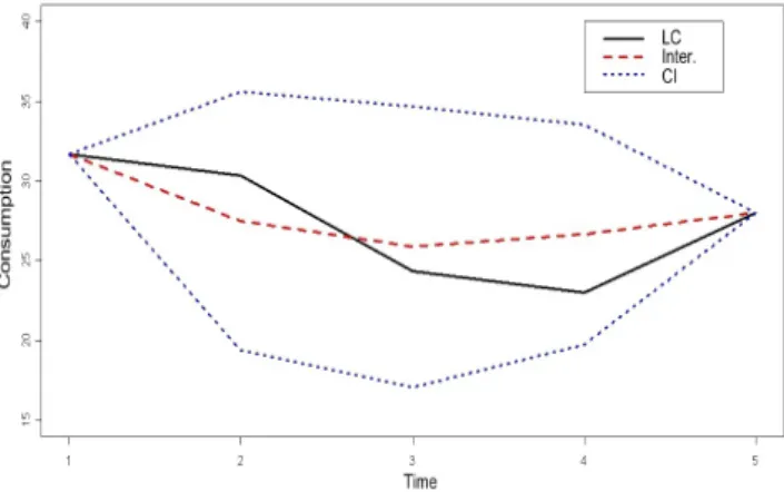
Suppose that temporal sampling has kept only 1 value over 4: onlyC(0) = 31.67 and C(4) = 28 were collected with a known energy ofE= 109.33kW hbetween 0 and 4. Knowing that the maximum power for this customer iscmax= 250kW,

7 linear optimization problems were solved: 2 for each the 3 intermediate points and one to find the estimated curve. The result is shown in Fig. 2: the original curve (LC) is repre-sented in plain style (black curve), the interpolation (Inter.) is presented with dashed style (red curve), and the envelopes (Env.) are presented with dotted style (blue curves).

Estimation on a time series.

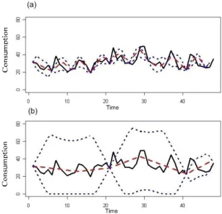
We now present the results of the approach on a daily time series, showing interpolation performed with two dif-ferent temporal sampling rates. In these two experiments, sampling rates of 5 (Fig. 3(a)) and 20 (Fig. 3(b)) were used.

Figure 2: Naive estimation and envelope between two selected points

Figure 3: Naive time series estimation and envelope

Each chart of Fig. 3 shows the original time series (plain black line), the reconstruction using the Naive approach (dashed red line) and the envelope (dotted blue line). It is clear that for both sampling rates, the estimated curve is close to the original one. We also note that the higher is the sampling rate, the larger is the envelope.

However, if sampling rates are chosen using an optimiza-tion technique that gives a larger sampling rate to time series which lightly fluctuate, the envelope in this case gives a very pessimistic estimation of errors. In fact, this approach does not provide any probability that a time series is inside the envelope since there is no underlying stochastic model. The second approach we propose, based on a stochastic model, provides such a probability in the form of a confidence inter-val.

The idea behind this second interpolation approach using a stochastic process is that fluctuations in consumption are random. Indeed, variations in an electric power consumption time series are induced by the start of a domestic activity such as meal preparation, launch of the washing machine, turn off of an electric heater, etc. Transitions between these activities can be modeled by a Markov process [6]. Even if it is hardly feasible to have a precise view of what this process should be on the basis of day-to-day behavior of each indi-vidual, this justifies the existence of randomness in the time series. As it is usually done, we presuppose that the global effect of all small fluctuations can be summarized by Brown-ian fluctuations. Moreover, an electric consumption is always a non-negative number, leading us to use a non-negative pro-cess with Brownian behavior. The simplest of them all is the so-called geometric Brownian motion (see below) which is also the basic model for the evolution of assets in mathematical finance.

2.2.1

Time series reconstruction and error estimation

C(t) =C(ta) exp(ρt+βBt1),

where B1 _{is a one-dimensional standard Brownian motion.}

Furthermore, e(t) is the consumed energy corresponding to the momentt(integral value att), hence

de(t) =C(t)dtore(tb)−e(ta) =

Z tb

ta

C(t)dt. RemindC(ta),C(tb), e(ta) ande(tb) are known. It is

there-fore difficult to simulate such a process since a stochastic be-havior is antonymous to deterministic limit conditions. The usual techniques are useless here because they involve in-tractable computations. We borrowed an idea from [5] which consists in constructing a simpler process which is relatively easy to simulate. We take into account the limit conditions and then use the Girsanov theorem. The detailed working of this problem’s solution is available as supplementary mate-rial [3].

For any functionf defined on [ta, tb], the solution is given

by the following expression of expectation: E " f(C, e) C(ta) e(ta) ! , C(tb) e(tb) !# =E[f(Q 0 , R0)M(Q0, R0)] E[M(Q0_{, R}0_)] (1) WhereM is a function depending on two processesQ0 and R0 _{that can be easily simulated.}

To estimate the time series between two sampled pointsta

and tb, we use a constant function defined by f(X) = X.

Then, Equation 1 becomes E " C(t) C(ta) e(ta) ! , C(tb) e(tb) !#

To compute the variance (error estimation), we use the func-tionf(X) = (X−E(X))2 asV ar(X) =E[X−E(X)2], and we apply this function to the result given by Eq.( 1):

E " (C(t)−E(C(t))2 C(ta) e(ta) ! , C(tb) e(tb) !# (2) To estimate parameters of the stochastic approach, we use the known properties of the geometric Brownian motion. Indeed,

we know that ln(C(t)) between ta and tb follows a normal

distribution with a mean equal to ρ(tb−ta). Therefore, we

estimateρusing: ρ= 1

(tb−ta)

(ln(C(tb))−ln(C(ta))).

Parameterβcan be estimated from historical data or using simulations. For instance, we can compute an approximation of the time series using a second-degree polynomial that re-spects the constraint of energy. We can perform several sim-ulations with different values ofβto get one that approaches the polynomial. In our experiments, we have fixed parameter βto be equal to 1.

2.2.2

Example

We study the same time series as that used for the Naive approach, i.e a day curve of 48 measurements (measurements every 30 minutes).

Estimation between two collected values.

We use the same sub-time series as in the naive approach with 5 values:

C={31.67,30.33,24.33,23,28}

we recall that the sampling rate is 4. We seek to interpolate the time series betweenC(0) = 31.67 and C(4) = 28 know-ing the energy consumed E = 109.33KW h (e(ta) = 0 and

e(tb) =E). We used the following parameters for the

condi-tioned geometric Brownian motion: β= 1, ρ= 1

(tb−ta)

(ln(C(tb))−ln(C(ta))) = 0.62.

Fig. 4 shows the result of interpolation (Inter.) represented by the red dashed curve. The envelope of standard devia-tion around this interpoladevia-tion (+/- one standard deviadevia-tion) is represented by the blue dotted curve (CI). The black curve (LC) is the original curveC.

Figure 4: Brownian stochastic estimation between two se-lected points

Estimation on a time series.

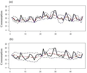
We applied the stochastic approach to interpolate the day time series passing through selected points. Fig. 5 shows the

result of interpolation using two sampling rates. A first sam-pling rate of 5 is applied and results are shown in Fig. 5(a). A second sampling rate of 20 is shown in Fig. 5(b).

Figure 5: Brownian stochastic time series estimation and con-fidence interval

Each chart of Fig. 5 shows the original time series (plain black line), the reconstruction using the brownian stochastic approach (dashed red line) and the confidence interval (dot-ted blue line). As in the Naive approach, it is clear that for both sampling rates, the estimated time series is close to the original one. Moreover, unlike the Naive approach, the enve-lope does not seem to be pessimistic in the example. Indeed, we have an analytical expression (eq. (2)) that allows us to compute a real confidence interval.

3.

EXPERIMENTAL STUDY

Several experiments have been carried out both on syn-thetic and real data. Some experiments show that taking into account the integral decreases the reconstruction error compared to a simple linear interpolation technique: these experiments, based on on a small dataset of real data, are not reported here but are available as supplementary mate-rial in [3].

We report in this paper extensive experiments carried out on a real data set of 1000 electric meters, each meter mea-suring the electric power consumption of one customer. The data set consists of 1000 times series with one measure every 10 minutes during one day (144 measurements per meter per day). It has been used to assess the efficiency of the approach in the case of small domain estimation: we estimate the ag-gregated sum of daily time series for a small sub-population, i.e., a small subset of meters.

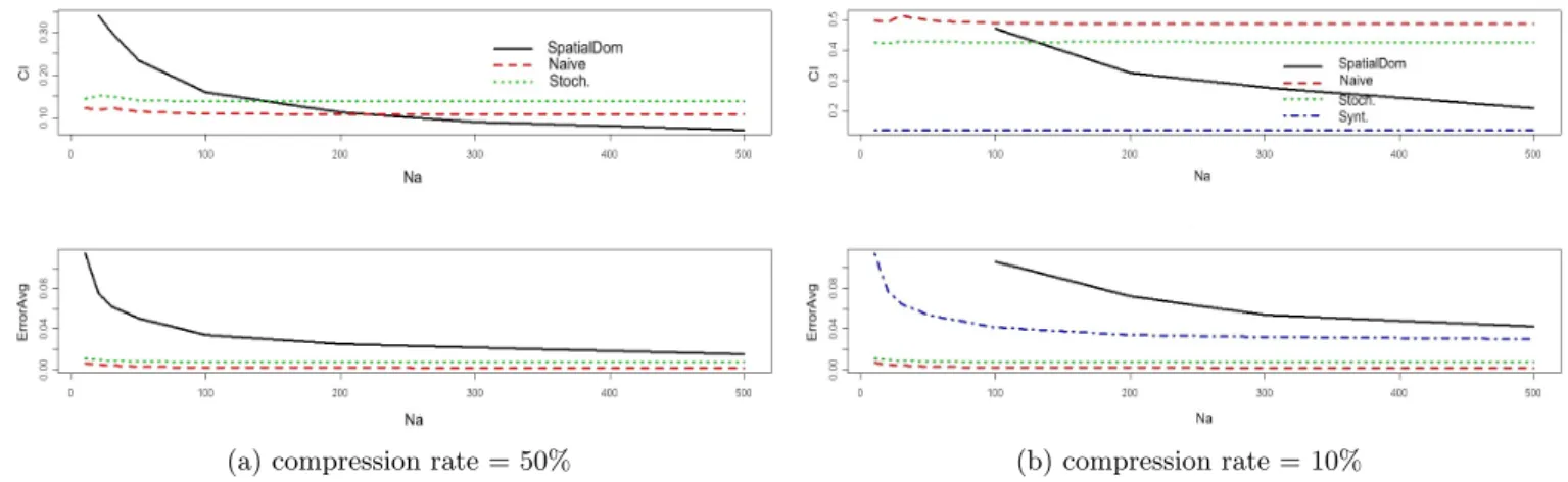
The reported experiments show the results for two compres-sion rates (50% and 10%) and compare the temporal sampling approach (data are collected from all meters but not at all timestamps) with a spatial random sampling approach (data are collected only from a random sample of meters but at all timestamps). A compression rate of 10% (resp. 50%) means: (1) in the spatial approach the size of the random sample of meters is 100 (resp. 500); (2) in the temporal approach only one value every 10 (resp. 2) timestamps is kept.

The reported experiments show the average relative error between the estimated aggregated time series (ErrorAvg in Fig. 6a and 6b ) and the associated relative confidence interval (CI). The confidence intervals are defined as follows:

• spatial sampling: the 68% Horvitz-Thompson confidence interval

• temporal sampling with naive estimation: sum of indi-vidual sizes of the envelopes withαmin adjusted with

X= 0.68

• temporal sampling with stochastic estimation: sum of individual confidence intervals corresponding to +/- 1 standard variation

The experiments were carried out over different sizes of small domainsNa on which the aggregated time series were

computed. These domains are of size

Na∈ {10,20,30,50,100,200,300,400,500}

In order to have an idea of the average behavior for each domain size, 100 Monte Carlo simulations were made.

In the case of spatial sampling with a 10% compression rate, it may happen with very small domains that either no or a very small number of time series belong simultaneously to the sample and to the domain. In this case, another estimator is used (called ’synthetic’ estimator) which uses the whole sample instead of the small domain selection on the sample. This leads to the ’Synt.’ blue curve in Fig. 6b.

Fig. 6a reports the results with a compression rate of 50%, i.e. the time series are summarized by dividing by 2 their original size. The lower chart shows the average relative er-ror (measured in terms of Sum of Square Erer-rors (SSE)) over the size of the domains on which the aggregation is done. The upper chart shows the size of the confidence intervals as defined above. As one can see, temporal sampling in this case always gives a better estimation than spatial sampling. The Naive estimation appears to be a little better than the stochastic brownian approach. As for the confidence interval, the naive envelope is better than the brownian confidence interval, but we recall here that there is no probabilistic in-terpretation to the confidence interval of the naive approach. With no surprise, the confidence interval of the spatial sam-pling decreases when the domain size increases, and ends up to be better than the ones of temporal sampling.

Fig. 6b reports the results with a compression rate of 10%, i.e. the time series are summarized by dividing by 10 their original size. We observe that temporal sampling with Naive estimation still gives the best estimation. The Brownian stochastic estimation is also very good. The results show clearly that temporal sampling is better than spatial sam-pling for small domains, even when the size of the domain is 500 (half of the dataset here). Note that for small domains the ’synth’ spatial sampling estimator is always better than the standard Horvitz-Thompson one. As for the confidence interval, the temporal sampling confidence intervals are al-most always worse than the spatial sampling one: this can be explained by the fact that the confidence interval in the tem-poral sampling approach is pessimistic since it is computed by adding confidence intervals of every time series which are aggregated (all time series are considered separately: errors cannot cancel each other out in the confidence interval com-putation).

(a) compression rate = 50% (b) compression rate = 10% Figure 6: Spatial sampling Vs. Temporal sampling

4.

CONCLUSIONS AND PERSPECTIVES

Within the context of storing a summarized version of a large set of time series issued from distributed sensors, we have shown that in many cases the time series may be ob-served at different timestamps. This is a problem when one wants to compute aggregates over a subset of the time series. The standard solution is to interpolate missing values and ag-gregate interpolated values. In the case where both the time series and their integrals are known, we have proposed two new approaches which take into account this information and provides also a confidence interval. Experiments have been re-ported to show that these approaches are efficient for estima-tion of the aggregated sum of time series over small domains, in particular if there are compared to another approach for summarizing distributed time series which naturally keeps all the time series values: the collection of a random sample of the sensors. This work opens several perspectives which are worth studying, mainly:

• develop the naive estimation method which gives a very accurate estimation, in order to provide a probabilistic confidence interval

• take into account possible correlations between values issued by different sensors

• propose an hybrid approach combining temporal and spatial sampling with a probabilistic confidence interval

5.

REFERENCES

[1] G.C. Cawley, N.L.C. Talbot, R.J. Foxall, S.R. Dorling, D.P. MandicHeteroscedastic kernel ridge regression, Neurocomputing Volume 57, March 2004, Pages 105-124.

[2] G.C. Cawley, N.L.C. Talbot, R.J. Foxall, S.R. Dorling, D.P. Mandic Unbiased estimation of conditional variance in heteroscedastic kernel ridge regression, Proceedings of the European Symposium on Arti6cial Neural Networks (ESANN-2003), Bruges, Belgium, April 2003.

[3] R.Chiky, L. Decreusefond and G.H´ebrail. Supplementary material, available at

http://www.infres.enst.fr/~chiky/edbt2010.

[4] R.Chiky and G.H´ebrail. Summarizing Distributed Data Streams For Storage in Data Warehouses. DaWak 2008 Turin (Italy).

[5] B. Delyon et Y.Hu. Simulation of conditioned diffusion and application to parameter estimation. Stochastic Processes and their Applications, Volume 116, Issue 11, November 2006.

[6] J.B. Durand, L. Bozzi, G. Celeux, C. Derquenne. Analyse de courbes de consommation ´electrique par chaˆınes de Markov cach´ees. Revue de Statistique Appliqu´ee, 52 no. 4 (2004), p. 71-91.

[7] J. Gehrke, F. Korn, and D. Srivastava. On computing correlated aggregates over continual data streams. In Proceedings of the 2001 SIGMOD Conference, pages 13-24, 2001.

[8] A. Gilbert, Y. Kotidis, S. Muthukrishnan, and M. Strauss. Quicksand : Quick summary and analysis of network data. Dimacs technical report, Department of Computer Science, Brown University, 2001.

[9] G. M. Phillips. Interpolation and Approximation by Polynomials. Springer; first edition (April 8, 2003). [10] J. N. K. Rao. Small Area Estimation. Hardcover, 344

pages, ISBN: 978-0-471-41374-5, January 2003. [11] Y. Till´e. Sampling Algorithms. Springer Series in

Statistics, 2006, XI, 216 p., Hardcover, ISBN: 978-0-387-30814-2.

[12] S. Weisberg. Applied Linear Regression. Third Edition published by Wiley/Inter science in 2005.