An investigation of train drag reduction using sub-boundary layer vortex generators on a simplified intermodal well car geometry

2017

An investigation of train drag reduction using

sub-boundary layer vortex generators on a simplified

intermodal well car geometry

Alexander Montgomery Peters

Iowa State University

Follow this and additional works at:https://lib.dr.iastate.edu/etd Part of theAerospace Engineering Commons

This Thesis is brought to you for free and open access by the Iowa State University Capstones, Theses and Dissertations at Iowa State University Digital Repository. It has been accepted for inclusion in Graduate Theses and Dissertations by an authorized administrator of Iowa State University Digital Repository. For more information, please [email protected].

Recommended Citation

Peters, Alexander Montgomery, "An investigation of train drag reduction using sub-boundary layer vortex generators on a simplified intermodal well car geometry" (2017).Graduate Theses and Dissertations. 16193.

generators on a simplified intermodal well car geometry

by

Alexander M. Peters

A thesis submitted to the graduate faculty

in partial fulfillment of the requirements for the degree of MASTER OF SCIENCE

Major: Aerospace Engineering

Program of Study Committee: Leifur Leifsson, Major Professor

Richard Wlezien Peng Wei

The student author, whose presentation of the scholarship herein was approved by the program of study committee, is solely responsible for the content of this thesis.

The Graduate College will ensure this thesis is globally accessible and will not permit alterations after a degree is conferred.

Iowa State University Ames, Iowa

2017

TABLE OF CONTENTS

2.1 Freight Train Aerodynamics . . . 5

2.2 Other Heavy Vehicles . . . 7

2.2.1 High-Speed Trains . . . 7

2.2.2 Tractor Trailers . . . 8

2.3 Vortex Generators . . . 9

CHAPTER 3. COMPUTATIONAL FLUID DYNAMICS MODELING 12 3.1 Geometry . . . 12

3.1.1 Geometry Scaling . . . 13

3.2 Simulation Domain . . . 17 3.2.1 Meshing . . . 18 3.2.2 Flow model . . . 18 3.3 Validation Case . . . 20 3.3.1 Mesh . . . 22 3.3.2 Results . . . 22

CHAPTER 4. COMPUTATIONAL RESULTS . . . . 26

4.1 Grid Independence Studies . . . 26

4.2 Individual Configuration Results . . . 28

4.2.1 Locomotive and 2 Intermodal Cars (L2IM) . . . 28

4.2.2 Locomotive and Two IM Cars and One set of Vortex Generator per IM Car (L2IM+1VG) . . . 28

4.2.3 Locomotive and Two IM Cars and Two sets of Vortex Generator per IM Car (L2IM+2VG) . . . 33

4.2.4 Locomotive and Two Intermodal Cars and Two sets of Large Vortex Generator per IM Car (L2IM+2LVG) . . . 33

4.3 Comparisons between Configurations . . . 38

CHAPTER 5. CONCLUSION . . . . 45

REFERENCES . . . . 48

APPENDIX A. CFD VALIDATION CASES . . . . 52

APPENDIX B. LOCOMOTIVE SIMULATIONS WITH SYMMETRY PLANE . . . . 57

LIST OF FIGURES

Figure 1.1 An intermodal well car with double stacked intermodal containers

(White (2015)) . . . 2

Figure 2.1 Wheeler vortex generator, Wheeler (1991) . . . 11

Figure 3.1 Simplified locomotive geometry standard 3-view (dimensions in meters) . . . 13

Figure 3.2 Intermodal geometry standard three-view (dimensions in meters) 14 Figure 3.3 Wishbone vortex generator geometry . . . 16

Figure 3.4 Simulation domain of a locomotive and two intermodal cars . . . 17

Figure 3.5 Sample meshes for three of the cases investigate . . . 19

Figure 3.6 Vortex generator mesh . . . 20

Figure 3.7 GTS geometry . . . 21

Figure 3.8 GTS domain . . . 21

Figure 3.9 Sample mesh for the ground transportation system . . . 23

Figure 3.10 Ground transportation system mesh independence study . . . 23

Figure 3.11 Streamlines of the wake behind the GTS . . . 24

Figure 3.12 Normalized velocity profiles in the wake of the GTS . . . 25

Figure 4.1 Mesh independence studies for the scaled trains . . . 27

Figure 4.2 Velocity contours along the flow direction at the midplane . . . . 29

Figure 4.4 Velocity contours along the flow direction at the midplane of

L2IM+1VG . . . 31

Figure 4.5 Streamlines along L2IM+1VG . . . 32

Figure 4.6 Velocity contours along the flow direction at the midplane of L2IM+2VG . . . 34

Figure 4.7 Streamlines along L2IM+2VG . . . 35

Figure 4.8 Velocity contours along the flow direction at the midplane of L2IM+2LVG . . . 36

Figure 4.9 Streamlines along L2IM+2LVG . . . 37

Figure 4.10 Line probe locations . . . 38

Figure 4.11 Velocity profiles along all four configurations (locations 1 through 4) . . . 41

Figure 4.12 Velocity profiles along all four configurations (locations 5 through 8) . . . 42

Figure 4.13 Overall Drag Comparison . . . 43

Figure 4.14 Train drag source comparisons . . . 43

Figure 4.15 The percent reduction in drag on the IM cars . . . 44

Figure A.1 Backwards facing step geometry (dimensions in meters) . . . 52

Figure A.2 Backward facing step mesh study . . . 53

Figure A.3 Backward facing step example meshes . . . 53

Figure A.4 Sensitivity analysis of turbulence models . . . 54

Figure A.5 Wall stress vs. distance from backwards facing step (m) for the Menter k-ω SST with κ= 0.492 . . . 55

Figure A.6 Geometry of the rectangular cut out simulation . . . 56

Figure A.7 Cp distributions experimental and CFD comparisons . . . 56

Figure B.2 Mesh study for a half domain L2IM . . . 59

Figure B.3 Velocity along the flow direction on the symmetry plane . . . 60

Figure B.4 Mesh study for a half domain L2IM+1VG . . . 60

NOMENCLATURE

Symbols

ρ Density, slugs

A Rolling Resistance per Ton

B Mechanical Resistance Dependent on Velocity per Ton

C Drag Coefficient per Ton

CD Drag Coefficient

Cp Pressure Coefficient

p Local Pressure, psi

p∞ Reference Pressure, psi

V Velocity, mph

V∞ Free Stream Velocity, mph

Abbreviations

CFD Computational Fluid Dynamics

DDES Delayed Detached Eddy Simulation

HST High Speed Train

IM Intermodal

L2IM+1VG Locomotive With two Intermodal Cars and one set of Vortex Generators per Car

L2IM+2LVG Locomotive With two Intermodal Cars and two sets of Large Vortex Ge-nerators per Car

L2IM+2VG Locomotive With two Intermodal Cars and two sets of Vortex Generators per Car

L2IM Locomotive With two Intermodal Cars RANS Reynold-Averaged Navier-Stokes

ACKNOWLEDGEMENTS

I would to thank those who advised and supported me as I worked on this research. In particular I would like to thank Dr. Richard Wlezien and Dr. Leifur Leifsson, without their guidance and advice I would never have made it this far. I would also like to thank Dr. Peng Wei for his instruction, patience, and for agreeing to be part of my committee. Special thanks to Wayne Kennedy, Spencer Maynes, and Walter Woodford whose first hand knowledge and expertise offered invaluable guidance to this project. I would also like to thank my family and friends especially my father and my fiancée who were both always there when I needed someone to talk to and supported me through out this work.

ABSTRACT

Railroad companies in the United States spent about $6.6 billion on diesel to move freight in 2015. One way to save money and reduce fuel consumption is to reduce the drag on the train. With the length of trains in the United States the drag due to the gaps between cars in the train is substantial. To reduce the drag between cars the intermodal well car was investigated. These cars carry intermodal containers often stacked two high. There were 12.2 million intermodal containers shipped in 2015, making the intermodal well car one of the most common cars in use. To avoid the need for major structural changes to the intermodal container wishbone vortex generators were investigated. Using steady Reynolds-Averaged Navier-Stokes simulations the flow field around a train consisting of a scaled and simplified locomotive and two intermodal cars was investigated. Sub-boundary layer vortex generators were then added to this model in two configurations. The first configuration added vortex generators to the rear of the intermodal cars, whereas the second configuration added vortex generators to both the front and rear of the intermodal cars. The vortex generators were sized according to two different boundary layer heights. The first height was found using flat plate turbulent boundary layer theory. The second used the boundary layer developed at the end of the first intermodal car. The addition of the smaller vortex generator showed a 2% drag reduction. While this reduction is close to the minimum accuracy of the simulation, the change in the drag on each car shows that further study is necessary to truly evaluate these devices. The larger vortex generators on the other hand show a 12% increase in the drag of the train.

CHAPTER 1.

INTRODUCTION

1.1

Motivation

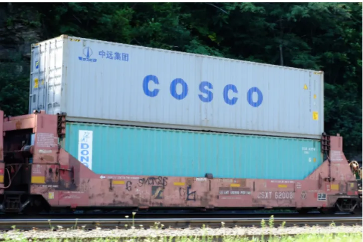
In the United States one of the most common ways to transport goods is by rail. Trains covered 35.8 billion miles to deliver freight in 2015. To move all this freight the the rail roads used approximately 3.7 billion gallons of diesel fuel, spending about 6.6 billion dollars (Anon, 2016b). Even a small improvement in fuel efficiency will have large effects on the amount of money spent on fuel and emissions from trains. One method to reduce fuel consumption is to reduce the drag on the train. A good place to reduce the aerodynamic drag may be improvements to the aerodynamic characteristics of intermodal containers. In 2015, 12.2 million intermodal containers were shipped by rail in the US (Anon, 2016b). These containers are usually shipped in what are called well cars and often stacked two containers high. An example of this is shown in Fig. 1.1. Many different methods could be investigated for drag reduction. One approach could be to add fairings to the intermodal containers. While this would likely be effective, it is not feasible due to the international standard that the intermodal containers are built to. Another method may be using vortex generators to couple to the wakes between cars. Vortex generators work by pulling relatively high energy air from the freestream back into the boundary layer. This high energy air can overcome adverse pressure gradient and is often used to re-attach flow along a body (Lin, 2002). This method has not been investigated on trains before to the authors knowledge.

Figure 1.1 An intermodal well car with double stacked intermodal containers (White (2015))

1.2

Challenges

Due to their size and shape trains can be difficult to aerodynamically investigate. Their modular nature requires a very clear objective since the order and spacing of cars will effect the flow features (Flynn et al., 2014). One of the challenges of reducing aero-dynamic drag is the cars themselves. Most freight cars are designed with an eye toward utility and construction cost rather than the aerodynamic drag on the train. The shear variety of cars can also be quite daunting.

Depending on the selected objective many different investigation methods are pos-sible. Each has its own challenges. The most direct is a full scale rundown test. This method of testing requires a long flat track, instrumented full size train, and a day with the required weather conditions. Another method is to use a wind tunnel. For the most accurate results a moving ground plane must be installed in the tunnel to avoid the ef-fects of the boundary layer that develops on the ground plane in the wind tunnel. Both of these methods are difficult, expensive and time consuming.

In this work, a commercial computational fluid dynamics (CFD) software, Star-CCM+, was used to analyze the flow past a freight train. The CFD work flow contains multiple interdependent steps. The first is creating the geometry and simulation

dom-ain, second is meshing the simulation domdom-ain, third is running the numerical simulation using the governing equations of fluid motion, and the fourth is post-processing the data. The geometry defines the shape of the and detail of the simulation domain. This is then fed directly into the mesher. The mesher attempts to discretizes the domain. The more detailed the geometry the more cells in the mesh and more realistically the simulation. The quality of the mesh is very important, cells that are stretched or skewed may give improper values that can either cause the simulation to crash or may drive the simulation to a non-physical result. Often the best way to improve the quality of a mesh requires an increase in the number of cells in the mesh. This creates a problem as well, the more cells in a simulation the longer it takes for the simulation to run. Even with the use of a high performance computing cluster the time it takes for a simulation to complete may become impractical. It is therefore important to balance the detail of the geometry with the quality and number of cells required for the simulation.

One of the biggest challenges when doing parametric studies with CFD is the need to show that the results are not within the possible error of the mesh itself. To do this mesh convergence studies must also be run for each geometry change. This means that for any geometry change there must be more than 3 simulation runs at different cell counts to show the change in the chosen characteristic value is negligible as the cell count increases. In this study the characteristic value is the drag coefficient.

1.3

Research Objective

The goal of this research is to investigate drag reduction on a train consisting of a locomotive and two intermodal cars. Since intermodal containers are built to an in-ternational standard any major changes to the containers themselves are unacceptable. Sub-boundary layer vortex generators have been utilized in this work to limit the im-pact of modifications on the containers. CFD was used to investigate the flow around

a locomotive and two intermodal cars with and without vortex generators. To complete the CFD simulations the cars have been simplified to reduce the required number of cells and the computational expense. These simplifications removed features such as the undercarriage on all the cars and the corrugations on the intermodal containers. These neglected features are unlikely change the large flow structures in the areas of interest, such as the gap between the intermodal cars.

1.4

Thesis Outline

The remainder of this thesis is organized as follows. Chapter 2 reviews works inves-tigating drag reduction techniques on heavy vehicles. This covers background on the aerodynamics of freight trains as well as how drag reduction methods from other heavy vehicles can be used to reduce the drag on freight trains. The geometry, mesh, and flow model selections used for the simulation of the flow past the locomotive and intermodal cars are covered in Chapter 3. This chapter also contains a validation verifying the se-lected mesh and flow models. Chapter 4 presents the results of the CFD simulations of trains both with and without vortex generators. The final chapter will draw conclusions from the results and suggest paths of future investigations. Appendix A contains further validation cases comparing different meshing and flow models. Appendix B describes observations found when attempting to simplify the train domain using a symmetry plane.

CHAPTER 2.

BACKGROUND

This chapter discusses current methods of aerodynamic drag reduction on freight trains and other heavy vehicles, as well as giving background on vortex generators.

2.1

Freight Train Aerodynamics

Since the early 1900s one of the primary ways to estimate the resistance on a train has been the Davis equation. This equation uses empirically derived coefficients to approximate the total resistance on a train. It states that the total resistance on the train is equal to the sum of the rolling resistance, the mechanical resistances due to velocity multiplied by the velocity, and the aerodynamic drag, ie the total resistance is

R=A+B ·V +C·V2, (2.1)

whereA includes the rolling mechanical resistance, B the mechanical resistances depen-dent on velocity, C is similar to the coefficient of drag, and V is the velocity of the train(Rochard and Schmid (2000); Schetz (2001)).

With the max velocity of a train being legally restricted to 80 mph in the United States (Anon, 2017b) much of the aerodynamic work on freight trains has focused on better predicting the resistance of the train, understanding the interactions of the train slipstream with either tunnels or other surroundings of the train, and understanding the risk of roll over due to crosswinds. While work has been done on better predicting the air resistance, little of this work has been applied to the design of new cars and locomotives.

Recently in the United Kingdom there has been discussion of increasing the top speed of freight trains. While passenger trains often move at higher speeds it was unclear how the bluffer bodies of freight trains would be impacted. One of the areas of the most concern is the effect that the slipstream of the train might have on the surrounding envi-ronment. Sterling et al. (2008) found, using a moving model facility, that the flow field around a freight train is very dependent on the loading efficiency of the cars. He also found that the train could cause high enough turbulence on a nearby platform to cause passengers waiting for their train to fall. The conclusions that Sterling et al. (2008) found were also found by Flynn et al. (2014) using a Delayed Detached Eddy Simula-tion (DDES), a time dependent simulaSimula-tion that uses unsteady RANS near the walls and Large Eddy Simulations in the freestream. This method simulates flow features more accurately than RANS but is less computationally expensive than Large Eddy Simulati-ons.

To reduce drag and consiquently the fuel consumption of trains containing intermodal cars (IM) Lai et al. (2008) created an aerodynamic loading assignment model that selects the best cars to fill when assembling the IM cars. Their model attempted to minimize the drag as a function of the gap lengths, loading options, and given characteristics of the train. Lai et al. (2008) used their method to analyze a route and believe that using this method they would be able to reduce the fuel consumption of the train and save $28 million a year. While this investigation uses drag coefficients to estimate the drag of the train rather than doing an aerodynamic test it shows that the coupling of wakes in the train can have a dramatic effect on the fuel consumption.

2.2

Other Heavy Vehicles

2.2.1 High-Speed Trains

With the higher velocity of a high speed passenger train (HST) the aerodynamic drag has more of an impact on the overall resistance on the train. To help mitigate this different methods have been investigated. This includes investigations into how to best investigate flow features. Zhang et al. (2016) found in both wind tunnel and CFD investigations that neglecting the ground plane and rotating wheels lead to a 6.8% underestimation of the total drag on the train. Zhang et al. (2016) also found that a moving ground plane without rotating wheels the underestimation was reduced to 6%. This shows that the discrepancy is mostly due to the boundary layer development along the ground plane.

Kwon et al. (2001) investigated different methods for creating the moving ground plane in wind tunnel tests. The methods they investigated were a rotating belt and tangential blowing system. Both methods were found to be effective. The rotating belt is similar to a treadmill run underneath the vehicle. This ’treadmill’ moves at the same speed as the incoming flow so as to avoid the development of a boundary layer. The tangential blowing system reduces the boundary layer along the wall by blowing air into the boundary layer along flow direction adding energy to the flow. Multiple slots may be needed for longer trains to avoid the boundary layer developing later in the train. This method may also be more effective for longer trains since it is less expensive than the rotating belt and is easier to modify for the length of a train.

To reduce the drag on an HST the cars themselves can be smoothed. Ido et al. (2001) showed in wind tunnel tests that smoothing the bottom of the train using bogie skirts and under bogie covers the drag coefficient could be reduced by approximately 30%. Since most HSTs are a consistent size on the outside the smoothing of the cars is a little easier. For long trains the smoothing is much more important near the front of the train.

As air flows along the train a boundary layer developes, and as the boundary layer grows the speed of the fluid near the car reduces. In their wind tunnel experiments Kwon et al. (2001) found that for a six-car train a cavity on the first car increased the drag by 14% while a cavity on the sixth car only increased the drag by 1.5%.

2.2.2 Tractor Trailers

Tractor trailers have used many methods to reduce fuel consumption in recent years. Those methods are of interest in this work since similar problems can be found on tractor trailers and freight trains.

One of the most effective and common devices currently on the market is the boattail flap. This device helps stabilize and close the wake behind the trailer. Storms et al. (2004) found a 28% reduction in the drag on the Ground Transportation System (GTS) when using this type of device. Multiple studies have investigated these flaps as well boattail plates, a similar device, on the GTS and more complex tractor trailer geome-tries and found similar results (Hyams et al. (2011); Storms et al. (2001); Storms et al. (2006)).

Another way to stabilize the wake behind the tractor trailer is base blowing. This method injects air into the flow to add energy to the wake reducing the size of the reci-rculation region. This method has been examined by a few groups using CFD showing considerable promise (Manosalvas et al. (2015); Englar (2001)). Englar (2001) claims to have reduced the drag on the GTS geometry by up to 50%. For this method to work a compressor or high pressure tank must be installed on the vehicle will increase the weight of the vehicle and careful planning is necessary to avoid using as much fuel compressing the air as saved by the system.

The gap between the tractor and trailer can also add drag to the vehicle. This is most problematic when a crosswind is experienced. Even for a straight on flow the distance

between the cab and trailer can greatly effect the drag. In shorter gaps the flow creates a symmetric eddy that stays inside the gap where as at larger gap values the eddy will oscillate from side to side. This oscillatory pattern creates an asymmetric flow which has more drag (Arcas et al., 2004). Most tractor trailers have cab extenders along the side of the cab extending into the gap between the cab and trailer. Storms et al. (2006) found that these devices did not have much effect when used in straight on flows, but adding the extenders improved the drag when a crosswind was experienced.

One of the solutions that is gaining interest on tractor trailers is the use of vortex generators both at the end of the cab and the end of the trailer. These devices are sold in the US by Airtab. They sell a modified Wheeler or wishbone style vortex generator and claim a 2 to 5% improvement in fuel economy (Anon, 2017a). Using CFD simula-tions Miralbes (2012) simulated a range of vortex generator types on a tractor trailer. He also claimed that using airtab like vortex generators could yield a 3.8% reduction on fuel consumption. To achieve this he arranged vortex generators along the trailing edge of both the cab and the trailer. The best results were found when using corotating vane style vortex generators with a 5% reduction in fuel consumption.

2.3

Vortex Generators

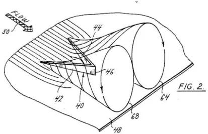
Vortex generators have long been used in aerodynamic designs. They are most com-monly seen on aircraft as a way to avoid flow separation. The vortex generators create a vortex that pulls high energy air out of the freestream into the boundary layer. This increases the energy in the boundary layer allowing it to overcome adverse pressure gra-dients. This work will focus on sub-boundary layer vortex generators also referred to as micro vortex generators. These vortex generators are buried within the boundary layer and their height is between 10 to 50% of the height of the boundary layer, this reduces the drag on the vortex generator.

There are many different types of sub-boundary layer vortex generators. Lin (2002) reviewed works on sub-boundary layer vortex generators. This review includes a com-parison of different vortex generator designs. In a backwards facing ramp investigation the most effective vortex generators were vanes followed by wishbone vortex generators. Lin (2002) also points out that the distance between vortex generators is very important especially with counter rotating vorticies. As the vortex expands down stream it will begin to interact with its neighbors. This can also be seen in other works (Hirt et al. (2012); Ashill et al. (2002)). To avoid this many studies have spaced their vortex gene-rators four heights apart or more (Lin (2002); Godard and Stanislas (2006)). This is also approximately the distance between the Airtabs when properly installed (Anon, 2016a). The vortex generator used in this study is similar to the one patented by Gary Wheeler in 1991. The V-shaped vortex generator, shown in Fig. 2.1, with the point of the V pointing along the flow direction. This vortex generator forces low speed flow up into the free stream causing a vortex that pulls free stream air into the boundary layer. This generator also works when the direction is reversed though it is less efficient. This loss of efficiency is due to the air falling down into the generator rather than be being pushed up by the generator (Wheeler, 1991). This is very important in our research since the IM containers can be placed on the car facing either direction and thus would need to have vortex generators installed on both edges.

CHAPTER 3.

COMPUTATIONAL FLUID DYNAMICS

MODELING

This gives the details of the computational fluid dynamics (CFD) model developed in this work. this includes a description of the geometry, meshing, and model. The chapter concludes with results of simulating the flow past Ground Transportation System (GTS) vehicle as a validation case of the CFD model.

3.1

Geometry

The CFD simulations involved in this investigation cover trains made up of a locomo-tive and two intermodal cars. Since the feature of interest of the simulation is the effect of vortex generators on the drag specifically across the gaps between intermodal cars and the wake behind the train simulations were run with and without vortex generators.

The base locomotive used in this simulation is the EMD SD70. The locomotive was de-featured until it became a rectangular prism with a ground clearance of 0.33 meters this corresponding to the distance from the bottom of the plow to the ground. The front side of the locomotive has been replaced with an ellipse with its minor axis set at the height of a normal SD70’s front deck with a major axis of 2.87 meters and a minor axis of 1.71 meters. There is also a fillet along the vertical portion of the front edges of 0.508 meters. The intent is to simplify and streamline the locomotive so that more cells can be applied to the IM cars and the gaps between them. Figure 3.1 shows a standard three-view of the simplified locomotive geometry.

Figure 3.1 Simplified locomotive geometry standard 3-view (dimensions in meters)

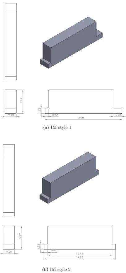
To reduce the cell count the intermodal (IM) car model was also simplified. The wheels and corrugations were removed and the sides of the intermodal containers were extended to be the same as the width of the well car. The expansion and the removal of the corrugations simplified the mesh in part by reducing the number of corners in the simulation. There are two different types of IM car involved in this investigated. The first IM car style has a longer tongue to connect to the cars before it, the second IM car style is symmetric about the middle of the IM container. Figure 3.2 shows both IM car geometries.

3.1.1 Geometry Scaling

To reduce the size of the domain the geometry was scaled with respect to the Reynolds number of 3.9 million. Table 3.1 shows how the scaling factor effects the velocity and thus the Mach number of the simulation. To avoid compressibility effects it is common practice to keep the Mach number below 0.3. Thus the smallest acceptable scale in this

2.90 5.92 0.90 2.21 19.26 1.32 (a) IM style 1 2.90 5.92 0.90 17.95 1.32 16.15 (b) IM style 2

Table 3.1 Train geometry scaling

Scaling Factor(%) Characteristic Length(m) Velocity(m/s) Mach Number

100 3.2 19.3 0.06 90 2.88 21.44 0.06 80 2.304 26.81 0.08 70 1.613 38.29 0.11 60 0.968 63.82 0.19 50 0.484 127.65 0.38

case is 60%. This smaller geometry allows for a mesh with fewer cells especially as the cells grow away from the geometry.

3.1.2 Vortex Generators

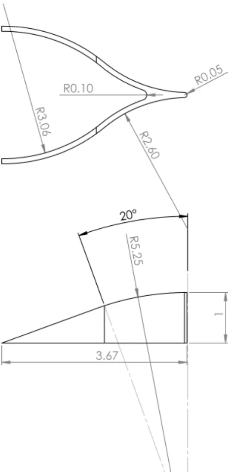
The vortex generators used in this study are specifically sub-boundary layer wishbone vortex generators. The geometry used in this simulation is very simmilar to the vortex ge-nerators used by Wendt and Hingst (1994). Figure3.3shows the geometry of a wishbone vortex generator with all the dimensions normalized to the height of the vortex genera-tor. Two different heights were used in this study.

The height of the smaller vortex generator was defined using flat plate boundary layer theory. The boundary layer was calculated using the length of a scaled IM car and the velocity of the simulation. The height of the vortex generator was then chosen to be 30% of the height of the boundary layer this gave a height of 3.4 cm. The height of the larger vortex generators was found by considering the height of the boundary layer on the locomotive and two intermodal car (L2IM) case at the end of the first intermodal car. The boundary layer at the given location was 1.114 meters tall. The height of the vortex generators for this location were then selected to be 10% of the this height.

The vortex generators were applied in two configurations. In both configurations the vortex generators where applied 1 cm from the rear face of the intermodal cars and had a 1 cm fillet along the lower edge. The generators where spaced four heights apart from center line to center line. The vortex generator arrays were along the top of the car and

R5.25 1 3.67 20° R0.05 R3.06 R0.10 R2.60 2.72

Figure 3.3 Wishbone vortex generator geometry

1.05 m down the sides of the car for the small generators. The large generators were placed along the top of the IM car and 1.5 meters down the side of the car, this extra half meter was allowed the addition of 1 more vortex generator. The tip of the generator pointed along the direction of the flow. In the second configuration a second set of vortex generators were applied in a mirror image of the first set across the center of the IM car. This new set of vortex generators pointed directly into the flow set 1 cm back from the front face of each IM car.

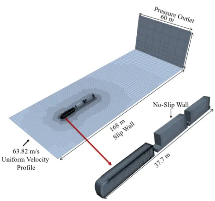
Figure 3.4 Simulation domain of a locomotive and two intermodal cars

3.2

Simulation Domain

A view of the simulation domain is given in Fig.3.4. The simulation domain is a box approximately 168 m long, 40 m tall, and 60 m wide. The scaled train is centered 30 m back from the front face, and 0.198 m above the ground plane. The front left right and top walls are all uniform velocity inlets at 63.8 m/s. The ground plane is a slip wall to simulate a moving ground plane, and the back wall is a pressure outlet.

To lower the required cell count and thus decrease the computational time required a symmetry plane was attempted. The plane was found to cause non-physical results for the locomotive with two IM cars (L2IM). An explanation of these results can be found in Appendix B.

3.2.1 Meshing

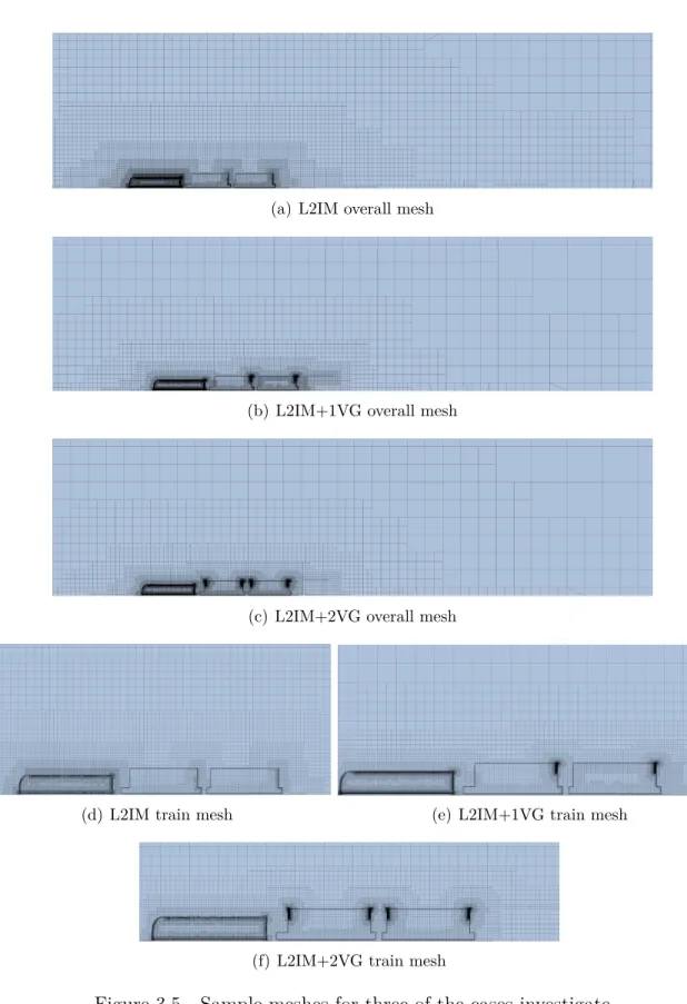
The Star-CCM+ trimmer mesher was used to mesh this simulation. The trimmer mesher requires much less memory to create a similarly sized mesh than the polyhedral mesher, allowing for the creation and simulation of larger meshes on the available com-putational hardware. The mesh is very course in the outer region and becomes finer as it approaches the train. Figure 3.5 shows an example of the mesh along the center line of the base geometry and both small vortex generator geometries.

The mesh is refined in the wake region of each car. This refinement extends 3 m from the rear face of each car. It specifies the maximum cell size and the growth rate in that region. The benefit of this wake region is that it helps place cells in the regions of interest specifically between the intermodal cars and the wake following the second intermodal car. The vortex generators have a very small target size, 1% of base, compared to the rest of the simulation. This is to try and capture the relatively small size of these devices and the vortices that they create. Figure 3.6 shows meshes for both vortex generator heights.

3.2.2 Flow model

To find the drag on the train a steady Reynolds-Averaged Navier-Stokes (RANS) simulation was used. The simulation was assembled and ran in Star-CCM+. The Menter k-ω SST turbulence model was selected. This model is common among CFD simulations since it gives many of the benefits of both the k- and the traditional k-ω models. One downside of this method is that it can over predict the size of separation regions. Some of the differences between the Menter k-ωSST and k-models were explored and the results can be seen in Appendix A. To increase the stability of the simulation the coupled flow solvers were used. This solver is usually used for compressible flows but due to the large flow separations that were expected in this flow the additional stability was expected to be beneficial.

(a) L2IM overall mesh

(b) L2IM+1VG overall mesh

(c) L2IM+2VG overall mesh

(d) L2IM train mesh (e) L2IM+1VG train mesh

(f) L2IM+2VG train mesh

(a) Small vortex generator (b) Large vortex generator

Figure 3.6 Vortex generator mesh

3.3

Validation Case

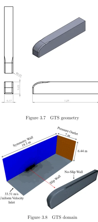
To validate the CFD models a simulation of the Ground Transportation System (GTS) model was run. This model has been run in both wind tunnel and CFD simu-lations (Manosalvas et al. (2015); Storms et al. (2001)). This simplified geometry was created by the Department of Energy to study methods to improve the fuel economy of tractor trailers. The model removes the gap between the tractor and trailer as well as removing all the features below the vehicle. It also give the trailer a more streamlined front. Further simplifications have been made for the ease of meshing the model. The wheels have been removed entirely and small fillets have been included on the sharp corners. These changes greatly simplify the meshing of the simulation. The GTS chosen for this simulation is a 6.5% scale representation similar to the one in Manosalvas et al. (2015), and can be seen in Fig. 3.7.

An example of the simulation domain can be seen in Fig.3.8. The simulation domain extends five vehicle lengths ahead of the GTS, nine vehicle lengths behind the GTS, and is both five vehicle lengths tall and wide. One of the side faces of the domain cuts the GTS in half vertically this face has been set as a symmetry plane. The front face is a velocity inlet at 33.5 m/s, the bottom face, or ground plane, is a slip wall to simulate a

Figure 3.7 GTS geometry

moving ground plane. The rear wall is a pressure outlet and the two remaining walls are also velocity inlets with a velocity of 33.5 m/s.

3.3.1 Mesh

Both the physics and mesh models are the same as for the train above. Figure 3.9

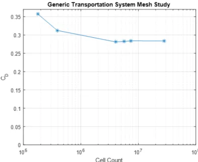
shows a sample mesh. The mesh is largest near the inlet and outlet and becomes finer as it approaches the GTS. The mesh is also finer in the wake of the GTS. This wake refinement extends 1.5 m from the back of GTS and can be seen in the slower growth rate in this area. A mesh independence study was run this simulation focusing on the drag coefficient as the number of cells increases. The drag coefficient of 0.2838 was found to be mesh independent up to 0.05% with 7.4 million cells as seen in Fig. 3.10.

3.3.2 Results

Since this model removes the support posts and wheels from below the GTS it is expected that the drag coefficient will be lower than that found in the wind tunnel experiments. Manosalvas et al. (2015) ran a similar steady RANS simulation and found that their drag coefficient was 0.3323 without the support struts or wheels. The CDfound

in the simulations studied in this paper are approximately 0.2824. The 15% difference between these results could be from the different methods in meshing, the different simulation software used, or in the use of a symmetry plane in this study.

Due to the bluntness of the geometry the drag is mostly due pressure drag rather than skin friction drag. This can be seen in both the stagnation region at the front of the vehicle and the large recirculation region at the rear of the vehicle. The recirculation in the wake behind the vehicle can be seen in the stream lines shown in Fig. 3.11. This figure shows the complex recirculation regions found in this wake.

Figure 3.12 shows slices of the wake for better comparison. Figure 3.12-a shows the velocity profile along the primary flow direction. It can be seen from this image that there

Figure 3.9 Sample mesh for the ground transportation system

is a large recirculation region. The stream lines in Fig. 3.11 show that the recirculation region is not just one recirculation but instead two recirculations that meet near the middle of the back face. Figure 3.12-b shows the vertical velocity on a plane parallel to the ground plane and 0.1768 m from the bottom of the GTS. This image show that the flow immediately after the face is moving up and further downstream is dominated by a downward moving flow. The final image shows the vertical velocity on plane paralleled to the ground and 0.05894 m from the bottom of the GTS. This plane shows a single lobe of upward moving air a little down stream of the GTS and air moving downward along the rear face of the GTS.

(a) Symetry plane

(b) Plane parallel to the ground 0.1768 m from the bottom of the GTS

(c) Plane parallel to the ground 0.05894 m from the bottom of the GTS

CHAPTER 4.

COMPUTATIONAL RESULTS

This chapter discusses the results of the locomotive and intermodal car simulations both with and with out vortex generators. The results are then compared with each other. The base case for this comparison is the locomotive with two intermodal cars (L2IM). The following cases are the L2IM with one small vortex generator location per car (L2IM+1VG), the L2IM with two small vortex generators (L2IM+2VG), and the L2IM with two large vortex generators (L2IM+2LVG).

4.1

Grid Independence Studies

Before the results of the simulations can be compared grid independence must be shown. Figure 4.1 show the studies for each of the geometries. While these studies do not show absolute convergence they do each show that the simulations are close to converged. The maximum relative error between the two finest meshes for any of the simulations is 3.1%. The relative error for the L2IM, L2IM+1VG, and L2IM+2VG are 1.6, 0.4, and 2.2% respectively. It can therefore be assumed that differences in the results greater than the relative error of the simulations are actually due to the differences in geometry rather than being in the possible error of the mesh. Since the overall drag coefficient decreases by 1% between L2IM and L2IM+1VG the benefits from the small vortex generators must be considered carefully. The 12% drag increase between L2IM and L2IM+2LVG is enough to fully reinforce this assumption for comparison between those configurations.

106 107 108 Cell Count 0 0.05 0.1 0.15 0.2 0.25 0.3 0.35 0.4 C D

L2IM Mesh Study

(a) L2IM mesh study

106 107 108 Cell Count 0 0.05 0.1 0.15 0.2 0.25 0.3 0.35 0.4 C D

L2IM+1VG Mesh Study

(b) L2IM+1VG mesh study

106 ₁₀7 ₁₀8 Cell Count 0 0.05 0.1 0.15 0.2 0.25 0.3 0.35 0.4 CD

L2IM+2VG Mesh Study

(c) L2IM+2VG mesh study

106 ₁₀7 ₁₀8 Cell Count 0 0.05 0.1 0.15 0.2 0.25 0.3 0.35 0.4 CD

L2IM+2LVG Mesh Study

(d) L2IM+2LVG mesh study

4.2

Individual Configuration Results

4.2.1 Locomotive and 2 Intermodal Cars (L2IM)

In Fig. 4.2 the velocity contour in the direction of the free stream is plotted along the midplane of the L2IM case. This figure shows that there is as expected a recircu-lation after each car and a separation on the first IM car. An interesting feature is the recirculation between the first IM car and the locomotive. This region has a very fast reverse flow from the impingement on the front face and the deck of the IM car. Another interesting result is the recirculation between IM cars 1 and 2. The rotational flow in this region would repeat multiple times in a full length train and any reduction in drag here could greatly improve fuel economy.

To better understand how the flow moves around the train in 3 dimensions Fig. 4.3

shows streamlines along the train. The streamlines show that the stagnation at the first intermodal car creates separation regions on both the top and sides of the car. There is also a vortex formed off the front of the first IM car that continues to rotate along the full length of the train. The gap between IM cars 1 and 2 can also be seen to be a recirculation region as is the wake behind the second IM car.

4.2.2 Locomotive and Two IM Cars and One set of Vortex Generator per

IM Car (L2IM+1VG)

Figure4.4shows the velocity along the flow direction on the midplane of the L2IM+1VG case. This flow looks very similar to the vehicle without vortex generators. The same separation and recirculation regions can be seen.

To clearly see the three dimensional aspects of the flow Fig.4.5shows the streamlines along the L2IM+1VG. This shows the very complex flow between IM cars 1 and 2. This flow seems to stay fairly slow but doesn’t seem to have a central vortex but rather multiple vorticies rotating both about the verticle and horizontal axes. It also shows

(a) F ull train (b) Gap b et w een Lo comotiv e and IM Car 1 (c) Gap b et w een IM c ars 1 and 2 (d) W ak e b eh ind IM car 2 Figure 4.2 V elo cit y con tours along the flo w direction at the midplane

(a) T op view (b) Sid e view Figure 4.3 Streamlines along L2IM

(a) F ull train (b) Gap b et w een lo comotiv e and IM car 1 (c) Gap b et w een IM c ars 1 and 2 (d) W ak e b ehind IM Car 2 Figure 4.4 V elo cit y con tours along the flo w direction at the midplane of L2IM +1 V G

(a) T op view (b) Sid e view Figure 4.5 Streamlines along L2IM+1V G

that IM car 1 has separation regions on both the top and the sides of the car. The separations seem to define the height of the boundary layer along both the top and side of the vehicle.

4.2.3 Locomotive and Two IM Cars and Two sets of Vortex Generator per

IM Car (L2IM+2VG)

Figure 4.6 shows the velocity in the flow direction at the midplane of L2IM+2VG. As before this profile shows the the freestream strikes both the locomotive and IM car 1. It also shows that the air recirculates after hitting IM car 1 and some of that flow hits the locomotive. The flow also recirculates between IM cars 1 and 2 and in the wake behind IM car 2.

Figure 4.7 shows the streamlines around the L2IM+2VG simulation. These stream-lines show that the flow between IM cars 1 and 2 is very complex. It also shows the 2 horizontal vortices in the wake region. Similar structures were seen in the Ground Transportation System verification study.

4.2.4 Locomotive and Two Intermodal Cars and Two sets of Large Vortex

Generator per IM Car (L2IM+2LVG)

The large vortex generators give a similar velocity contour as the earlier simulations as seen in Fig. 4.8. The most obvious difference is the amount of low velocity air being pushed up into the higher velocity boundary layer. This can be seen in the wake and at the top of the gap between IM cars 1 and 2. The separation on IM car 1 and the recirculations between the locomotive and IM car 1, IM car 1 and 2, and in the wake are also present in this simulation as they were in the previous simulations.

Figure 4.9 shows the streamlines around L2IM+2LVG. These streamlines show the large separations off the top and side of first IM car. The circulation along the side of the train seems to split with the flow that hits the vortex generators moving up towards the

(a) F ull train (b) Gap b et w een lo comotiv e and IM car 1 (c) Gap b et w een IM c ars 1 and 2 (d) W ak e b eh ind IM car 2 Figure 4.6 V elo cit y con tours along the flo w direction at the midplane of L2IM +2 V G

(a) T op view (b) Sid e view Figure 4.7 Streamlines along L2IM+2V G

(a) F ull train (b) Gap b et w een lo comotiv e and IM car 1 (c) Gap b et w een IM c ars 1 and 2 (d) W ak e b eh ind IM car 2 Figure 4.8 V elo cit y con tours along the flo w direction at the midplane of L2I M+2L V G

(a) T op view (b) Sid e view Figure 4.9 Streamlines along L2IM+2L V G

Figure 4.10 Line probe locations

top of the train and the flow that doesn’t hit that vortex generator moves down toward the bottom of the car. The streamlines also show the recirculation regions that are seen in the previous simulations.

4.3

Comparisons between Configurations

One of the best ways to see how the vortex generators effect the flow is to plot the velocity profile at given location along the train. Figure 4.10 shows the location of each velocity profile. Each profile is normalized to its height of 1.46 m and the freestream velocity. Figures 4.11 and 4.12 show these profiles at the given locations.

The first profile location is just behind where the first set of vortex generators are set on L2IM+2VG, this shows the beginning of the separation region. Profile locations 2 and 3 show the end of the separation bubble and the profile after reattaching the the IM car respectively. The fourth profile is just before the vortex generators set at the end of the car. Locations 5 and 6 are both above the gap between the IM cars. Location 7 is set in a similar location to the first showing how the flow interacts with the second IM car. Location 8 show the boundary condition after the flow has fully attached to the second IM car. The velocities in these contours are found at the nearest cell centers which leads to the abrupt changes seen in some of the contours when the mesh is not quite fine enough.

The velocity profiles show that the vortex generators are acting as expected. The L2IM+2VG case reattaches before either the L2IM or the L2IM+1VG. It also has an appreciably higher velocity near the wall in almost all of the cases. It is interesting to note that the L2IM+2VG and L2IM+1VG accelerate more across the gap than the L2IM case. This can be seen by comparing locations 4,5, and 6. As stated previously the L2IM+2VG case moves the fastest This may be due to the earlier reattachment that is implied at line probe 4.

Adding the larger vortex generators shows a much different velocity profile. The larger vortex generators re-attaches the first separation much faster than the other simulations. It also seems to have a much lower velocity near the top of the car as it crosses the gap as well as a very separated flow at location 8. At this location the other profiles have attached where as the large vortex generator has a large discontinuity. This may be because of the small separation caused by the generator at the front of the car.

Adding small vortex generators to the system can be seen to give positive results as seen in Fig. 4.13. The drag of the train seems to reduce by approximately 2% both the L2IM+1VG and L2IM+2VG cases. Adding the large vortex generators cause an increase in the drag coefficient (as seen in Fig.4.1). Figure4.13shows that the vortex generators themselves produce drag affecting the train. Figure 4.14 shows the percentage of the total train drag produced by each car and in the vortex generator cases the generators that have been added to the train. The drag addition from the vortex generators is most obvious in the large vortex generator case where the drag from the vortex generators is approximately 8% of the total drag of the train. In the L2IM+1VG and L2IM+2VG the drag produced by the vortex generators is more than offset by drag reduction on the intermodal cars leading to the 2% drag reduction in these cases when compared to the L2IM case.

Figure 4.15 compares relative differences in drag coefficient on each IM car when compared with the L2IM base case. The plot implies that the L2IM+1VG case reduces

drag only on the second car, approximately 13.6%, and shows an increased drag on the first IM car of approximately 3.5%. The L2IM+2VG case reduces drag on both cars by a much smaller amount, approximately 3.2% on the first IM car and 0.5% on the second IM car. The exact nature of the drag reduction requires further investigation due to the limitations of the simulations. The current train configuration may be masking some of the potential benefit of these devices since the first IM car is experiencing a direct impingement of the freestream and the second IM car has the large separation region behind it. These large drag regions may be dominating the drag experienced by each car.

-0.4 -0.2 0 0.2 0.4 0.6 0.8 1 1.2 Velocity 0 0.1 0.2 0.3 0.4 0.5 0.6 0.7 0.8 0.9 1 Position

Velocity Profile Line Probe 1 L2IM

1 Small VG 2 Small VG 2 Large VG

(a) Velocity Profile at Line Probe 1

-0.4 -0.2 0 0.2 0.4 0.6 0.8 1 1.2 Velocity 0 0.1 0.2 0.3 0.4 0.5 0.6 0.7 0.8 0.9 1 Position

Velocity Profile Line Probe 2 L2IM

1 Small VG 2 Small VG 2 Large VG

(b) Velocity Profile at Line Probe 2

0.1 0.2 0.3 0.4 0.5 0.6 0.7 0.8 0.9 1 1.1 Velocity 0 0.1 0.2 0.3 0.4 0.5 0.6 0.7 0.8 0.9 1 Position

Velocity Profile Line Probe 3 L2IM

1 Small VG 2 Small VG 2 Large VG

(c) Velocity Profile at Line probe 3

0.3 0.4 0.5 0.6 0.7 0.8 0.9 1 1.1 Velocity 0 0.1 0.2 0.3 0.4 0.5 0.6 0.7 0.8 0.9 1 Position

Velocity Profile Line Probe 4 L2IM

1 Small VG 2 Small VG 2 Large VG

(d) Velocity Profile at Line probe 4

0.3 0.4 0.5 0.6 0.7 0.8 0.9 1 1.1 Velocity 0 0.1 0.2 0.3 0.4 0.5 0.6 0.7 0.8 0.9 1 Position

Velocity Profile Line Probe 5 L2IM

1 Small VG 2 Small VG 2 Large VG

(a) Velocity Profile at Line Probe 5

-0.2 0 0.2 0.4 0.6 0.8 1 1.2 Velocity 0 0.1 0.2 0.3 0.4 0.5 0.6 0.7 0.8 0.9 1 Position

Velocity Profile Line Probe 6 L2IM

1 Small VG 2 Small VG 2 Large VG

(b) Velocity Profile at Line Probe 6

-0.2 0 0.2 0.4 0.6 0.8 1 1.2 Velocity 0 0.1 0.2 0.3 0.4 0.5 0.6 0.7 0.8 0.9 1 Position

Velocity Profile Line Probe 7 L2IM

1 Small VG 2 Small VG 2 Large VG

(c) Velocity Profile at Line Probe 7

-0.2 0 0.2 0.4 0.6 0.8 1 1.2 Velocity 0 0.1 0.2 0.3 0.4 0.5 0.6 0.7 0.8 0.9 Position

Velocity Profile Line Probe 8 L2IM

1 Small VG 2 Small VG 2 Large VG

(d) Velocity Profile at Line Probe 8

L2IM 1SVG 2SVG 2LVG 0 0.05 0.1 0.15 0.2 0.25 0.3 0.35 C D C_D Breakdown by Car 0.315 0.309 0.309 0.350 Locomotive Intermodal Car 1 Intermodal Car 2 Vortex Generators

Figure 4.13 Overall Drag Comparison

(a) L2IM (b) L2IM+1VG

(c) L2IM+2VG (d) L2IM+2LVG

1 Small VG 2 Small VG 2 Large VG -5 0 5 10 15 ∆ C D [%] Change in C_D on IM 1 3.5 -3.2 3.4

1 Small VG 2 Small VG 2 Large VG

-10 0 10 ∆ C D [%] Change in C_D on IM 2 -13.6 -0.5 4.0

CHAPTER 5.

CONCLUSION

In this work, the flow past a 60%-scaled simplified-geometry train consisting of a locomotive and two intermodal (IM) cars was investigated using computational fluid dynamics simulations. Specifically Reynolds Averaged Navier Stokes simulations were used with the Menter k-ω SST turbulence model. Three configurations were studies: the simplified geometry (a streamlined locomotive without wheels and squared sides and two intermodal cars without wheels or corrugations) without vortex generators, the same geometry with vortex generators applied to the rear of the IM cars, and with the vortex generators at the front and rear of the IM cars. The vortex generators used in this study were wishbone style generators similar to those in Wendt and Hingst (1994). The height of the small vortex generators was chosen to be 30% of the height of the flat plate turbulent boundary layer with a length equal to the length of a single intermodal car. The height of the larger vortex generators was chosen as 10% of the size of the boundary layer measured at the rear of the first intermodal car. To validate the mesh and flow models used the Ground Transportation System was analyzed and compared to prior work.

The simulations were then compared to study the changes that adding vortex gene-rators would cause. To make this comparison a mesh convergence study was run for each configuration. The results of this investigation imply that the addition of small vortex generators to IM cars could reduce the drag on these cars. While these results show drag reduction of approximately 2% potentially translate to large savings for the railroads in the United States. The comparison also implies that there may be some benefit that is

being hidden by the current configuration. The large drag sources at the front of the first intermodal car and at the rear of the second intermodal car could be masking some of the potential benefit seen in the gap between the first and second intermodal cars. The large vortex generator simulation showed an increase in total drag on the train. This total comes from both an increase in drag on the intermodal cars themselves and in drag from the large vortex generators being attached to the train. The difference in results between the large and small vortex generators show that careful design of size of the vortex generators should be considered when using these devices.

To better understand the results of adding vortex generators to the IM cars a few studies can be investigated. A comparison of the small vortex generators and a surface roughness model can be compared to see if the shape of the small vortex generators is actually causing the benefit. Simulations including more than two intermodal cars could be run to better understand the benefits of the vortex generators both as the train lengthens and in the gaps between cars. Parametric studies may also be run to show what effects train speed, vortex generator size, and vortex generator location and spacing may have on train drag. This would allow for a better understanding of how the vortex generators effect the flow individually and as an array. Leading to better application of the vortex generators. Another important topic to look into would be the effect of crosswind. It is very rare that a train will have only straight on flow the vortex generators need to be able to at a minimum not increase the drag on the train in a crosswind and hopefully decrease it.

The simulation methods themselves can also be improved. While these simulations were run using steady RANS the averaging of the Reynolds stress terms tends to smear the vorticity in the simulations. Since the train and the vortex generators can be ex-pected to shed vorticies this smearing may be important to the simulation. The Delayed Detached Eddy Simulation method would be a good next step since it is a hybrid of the RANS and the Large Eddy Simulation methods. This time accurate simulation

would show the development and shedding of the vortices and may give more accurate descriptions of the flow field.

REFERENCES

Anon (2016a). Airtab Installation Instructions. Airtab.

Anon (2016b). Railroad facts. Office of Information and Public Affairs, Association of American Railroads, Washington, D.C.

Anon (2017a). Airtab fuel savers. online. Accessed: October 8th 2017.

Anon (2017b). Classes of track: Operating speed limits. 49 C.F.R Section 213.9.

Arcas, D., Browand, F., and Hammache, M. (2004). Flow structure in the gap between two bluff bodies. 34th AIAA Fluid Dynamics Conference and Exhibit.

Ashill, P., Fulker, J., and Hackett, K. (2002). Studies of flows induced by sub boundary layer vortex generators (sbvgs). 40th AIAA Aerospace Sciences Meeting and Exhibit. Englar, R. J. (2001). Advanced aerodynamic devices to improve the performance,

econo-mics, handling and safety of heavy vehicles. Technical report, SAE Technical Paper. Flynn, D., Hemida, H., Soper, D., and Baker, C. (2014). Detached-eddy simulation of the

slipstream of an operational freight train. Journal of Wind Engineering and Industrial Aerodynamics, 132:1–12.

Godard, G. and Stanislas, M. (2006). Control of a decelerating boundary layer. part 1: Optimization of passive vortex generators. Aerospace Science and Technology, 10(3):181–191.

Hirt, S. M., Zaman, K. B., and Bencic, T. J. (2012). Experimental study of boundary layer flow control using an array of ramp-shaped vortex generators. National Aeronautics and Space Administration, Glenn Research Center.

Hyams, D. G., Sreenivas, K., Pankajakshan, R., Nichols, D. S., Briley, W. R., and Whitfield, D. L. (2011). Computational simulation of model and full scale class 8 trucks with drag reduction devices. Computers & Fluids, 41(1):27–40.

Ido, A., Kondo, Y., Matsumura, T., Suzuki, M., and Maeda, T. (2001). Wind tunnel tests to reduce aerodynamic drag of trains by smoothing the under-floor construction. Quarterly Report of RTRI, 42(2):94–97.

Kwon, H.-b., Park, Y.-W., Lee, D.-h., and Kim, M.-S. (2001). Wind tunnel experiments on korean high-speed trains using various ground simulation techniques. Journal of Wind Engineering and Industrial Aerodynamics, 89(13):1179–1195.

Lai, Y.-C., Barkan, C. P., and Önal, H. (2008). Optimizing the aerodynamic efficiency of intermodal freight trains. Transportation Research Part E: Logistics and Transpor-tation Review, 44(5):820–834.

Lin, J. C. (2002). Review of research on low-profile vortex generators to control boundary-layer separation. Progress in Aerospace Sciences, 38(4):389–420.

Manosalvas, D. E., Economon, T. D., Jameson, A., and Palacios, F. D. (2015). Techni-ques for the design of active flow control systems in heavy vehicles. AIAA Aviation Forum.

Miralbes, R. (2012). Aerodynamic analysis of some vortex generator improvements for heavy vehicles. International Journal of Heavy Vehicle Systems, 19(4):355–370.

Rochard, B. P. and Schmid, F. (2000). A review of methods to measure and calculate train resistances. Proceedings of the Institution of Mechanical Engineers, Part F: Journal of Rail and Rapid Transit, 214(4):185–199.

Roshko, A. (1955). Some measurements of flow in a rectangular cutout. Technical report, California Institute of Technology, Pasadena.

Schetz, J. A. (2001). Aerodynamics of high-speed trains. Annual Review of fluid mecha-nics, 33(1):371–414.

Sterling, M., Baker, C., Jordan, S., and Johnson, T. (2008). A study of the slipstreams of high-speed passenger trains and freight trains. Proceedings of the Institution of Mechanical Engineers, Part F: Journal of Rail and Rapid Transit, 222(2):177–193. Storms, B. L., Ross, J. C., Heineck, J. T., Walker, S. M., Driver, D. M., Zilliac, G. G.,

and Bencze, D. P. (2001). An experimental study of the ground transportation system (gts) model in the nasa ames 7-by 10-ft wind tunnel. NASA Technical Report.

Storms, B. L., Satran, D. R., Heineck, J. T., and Walker, S. (2004). A study of reynolds number effects and drag-reduction concepts on a generic tractor-trailer. 34th AIAA Fluid Dynamics Conference and Exhibit.

Storms, B. L., Satran, D. R., Heineck, J. T., and Walker, S. M. (2006). A summary of the experimental results for a generic tractor-trailer in the ames research center 7-by 10-foot and 12-foot wind tunnels. NASA Technical Report.

Vogel, J. and Eaton, J. (1985). Combined heat transfer and fluid dynamic measurements downstream of a backward-facing step. Journal of heat transfer, 107(4):922–929. Wendt, B. J. and Hingst, W. R. (1994). Measurements and modeling of flow structure

in the wake of a low profile wishbone vortex generator. NASA Technical Report. Wheeler, G. O. (1991). Low drag vortex generators. US Patent 5,058,837.

White, J. (2015). Cosoco 40 foot container. Used Under the Creative Commons Attri-bution 2.0 Generic License.

Zhang, J., Li, J.-j., Tian, H.-q., Gao, G.-j., and Sheridan, J. (2016). Impact of ground and wheel boundary conditions on numerical simulation of the high-speed train aero-dynamic performance. Journal of Fluids and Structures, 61:249–261.

APPENDIX A.

CFD VALIDATION CASES

This appendix compares the turbulence models used. The validation cases were the traditional backwards facing step and a comparison to a rectangular cut out study done by Roshko (1955).

Backwards Facing Step

This two dimensional problem is traditionally used to evaluate a turbulence model. One of the characteristics that can be used for this verification is the point at which the flow re-attaches to the lower wall.

The specific Backwards Facing Step that was simulated can be seen in Figure A.1. This geometry has a 1 meter step height and a 5 meter overall tunnel height. The simulation is 30 meters long to give enough space for the flow characteristics to dissipate before hitting the pressure outlet at the far right face. The upper and lower walls are both non-slip walls. The inlet was a fully developed boundary layer with a freestream velocity of 1 m/s.

Figure A.2 Backward facing step mesh study

(a) Trimmer mesher

(b) Polyhedral mesher

Figure A.3 Backward facing step example meshes

Backwards Facing Step Physics and Mesh

The intent of this simulation was to compare turbulence models as well as meshing methods. The Menter K-ω SST is more common for flows with large separation regions similar to what is expect in the later stages of the work, it also can over estimate the size of the separation as can be seen in Figure A.2. The Trimmer and Polyhedral meshers were compared as well. No prism mesher was selected due to the small size of the cells when compared to size of the fully developed boundary layer. An example mesh of both the Trimmer and Polyhedral meshers can be seen in Figure A.3.

(a) K- (b) Menter K-ω SST

Figure A.4 Sensitivity analysis of turbulence models

To better understand how the turbulence models work and how the internal coeffi-cients could effect the simulation a Polyhedral mesh was used to test a sweep of each turbulence coefficient for both models. The resulting sensitivity plots can be seen in FigureA.4.

While running the sensitivity analysis it was found that increasing the κ term in the Menter K-ω SST model reduced the size of the simulated separation region. If the κ term is set to 0.492 the point of reattachment exactly matches that found by Vogel and Eaton (1985) this can be seen in Figure A.5.

Rectangular Cut Out

Much of this research will depend on how the physics models act with the seperation and re-attachment between cars. To better understand the flow in this region simulations were created to compare with the work of Roshko (1955). Roshko explored a rectangular cut out with a variety of depths. For all depths the width of the cut out was wide enough

Figure A.5 Wall stress vs. distance from backwards facing step (m) for the Menter k-ω SST with κ= 0.492

to avoid any effects from the edges of the cutout. This allowed the simplification of the simulation to a 2D region. FigureA.6 shows the geometry of the rectangular cut out.

To compare to the results in Roshko (1955) the coefficient of pressure along the bottom plate was plotted. The coefficient of pressure can be found according to

Cp =

p−p∞ 1 2ρV∞2

, (A.1)

where p is the local pressure, p∞ is the reference pressure taken 1 in upstream of the

rectangular cut out,ρis the density, andV∞is the freestream velocity. ACpdistributions

for a depth of 3.5 inches is plotted below. These plots show range cell counts for both the K-epsilon and the K-omega turbulence models. Figure A.7 shows a mesh study compared to the experimental results found by Roshko. The results closely follow the trends of the experimental results improving as the cell count increases.

Flo w Pressure Outlet 36 in 4 in 1

Figure A.6 Geometry of the rectangular cut out simulation

APPENDIX B.

LOCOMOTIVE SIMULATIONS WITH

SYMMETRY PLANE

The addition of a symmetry plane was investigated in both the L2IM and L2IM+1VG. These models were the same as the full domain model except the model was cut in half by one of the domain walls. This wall was then set as a symmetry plane. Figure B.1

shows the half domain model of the L2IM.

This model used the same mesh and physics setting as the mesh and physics settings as the full domain tested in the main section of the thesis. The symmetry plane was originally included as an extension of the GTS simulations that were run. It was believed that if the plane worked for the GTS then it should work for the L2IM. The benefit of the symmetry plane is that it would allow the simulation to run faster due to a mesh that was half the size required for the full domain.

Figure B.2 shows mesh independence studies for both the L2IM and L2IM+1VG. These studies were suspended once the problems with the symmetry plane were found. The L2IM+VG mesh study seems to have been approaching its asymptote at about CD = 0.4. This could be caused by a few things. In Figure B.3 the velocity along the

flow direction for the half domain L2IM are shown at the symmetry plane.

The 2 most interesting differences between this velocity field in the full domain are in the gap between IM cars 1 and 2. There is a lobe of low speed flow extending into the boundary layer above the train. This flow doesn’t seem to curve to the wall as would be expected in reality but seems to sit a little up stream of the second intermodal car. The other is the reversed flow on the ground plane below the first intermodal car.

Figure B.1 L2IM half domain

This reversed flow seems to be separated from the rest of the flow in the gap. Another qualitative observation is the flow behind the second IM car seems to have less reversed flow than the gap between cars as well as being raised farther off the ground than what is seen in the full domain simulations.

The problems with this simulation could be caused by flow into the symmetry plane. One of the base assumptions that must be made when using a symmetry plane is that the flow into the plane is negligible. As the full domain simulation showed the flow between the cars has multiple vortices some of which may cross the center line. Since this flow is not negligible the symmetry plane is an invalid assumption.

While the flow without the vortex generators is obviously not physical when adding the vortex generators to the rear of the IM cars the simulation improved. This can be seen in the Mesh Independence Study in Figure B.4. The changes in mesh size seem to move more smoothly to approximately 0.31. This also is very similar to the drag coefficient found in the full size domain. The flow field shown in FigureB.5 also looks

105 106 107 108 Cell Count 0 0.05 0.1 0.15 0.2 0.25 0.3 0.35 0.4 C D L2IM W/ Symmetry

Figure B.2 Mesh study for a half domain L2IM

much more physical. The shape and values are similar to those shown in Figure4.4. This implies that the vortex generators are stabilizing the flow in the gap avoiding oscillations that would cause the flow to cross the symmetry plane.

Figure B.3 Velocity along the flow direction on the symmetry plane