Multi-Robot Tracking of a Moving Object
Using Directional Sensors
Manuel Mazo Jr., Alberto Speranzon, Karl H. Johansson
Dept. of Signals, Sensors & SystemsRoyal Institute of Technology SE-100 44 Stockholm, Sweden
[email protected],{albspe,kallej}@s3.kth.se
Xiaoming Hu
Dept. of Mathematics Royal Institute of Technology SE-100 44 Stockholm, SwedenAbstract— The problem of estimating and tracking the motion of a moving target by a team of mobile robots is studied in this paper. Each robot is assumed to have a directional sensor with limited range, thus more than one robot (sensor) is needed for solving the problem. A sensor fusion scheme based on inter-robot communication is proposed in order to obtain accurate real-time information of the target’s position and motion. Accordingly a hierarchical control scheme is applied, in which a consecutive set of desired formations is planned through a discrete model and low-level continuous-time controls are executed to track the resulting references. The algorithm is illustrated through simulations and on an experimental platform.
I. INTRODUCTION
Multi-robot systems are used in many situations in order to improve performance, sensing ability and reliability, in com-parison to single-robot solutions. For example, in applications like exploration, surveillance and tracking, we want to control a team of robots to keep specific formations in order to achieve better overall performance. Formation control is a particularly active area of multi-robot systems, e.g., [1], [2], [3], [4], [5]. Most of the work in the literature, however, is focused on the problem of designing a controller for maintaining a preassigned formation. The issue of sensors limitations seems to be more or less overlooked. In this paper we consider the problem of localizing and tracking a moving object using directional sensors that are mounted on mobile robots. When the range is far and the resolution becomes low, many visual sensors are in effect reduced to only directional sensors, since the depth information is then hard to recover. In situations like this, sensing and estimation become central and an integrated solution for control and sensing desirable. Since we need to have sufficient separation for the sensor channels, it is reasonable that we mount the sensors on different robots. Thus the goal of the control design is not only that the robots should track the target, but also that the robots should coordinate their motion so that the sensing and localizing of the target is not lost.
The main contribution of our work is a hierarchical al-gorithm for localizing and tracking a moving target. We study a prototype of a distributed mobile sensing system, namely, a team of two nonholonomic robots with sensors for the environment. These tracking robots have hard sensor constraints, as they can just obtain relative angular position
of the target within a limited field of vision, and relative positions of each other within short distance. Our solution provides a cooperative scheme in which the higher level of the algorithm plans a formation for the robots to follow in order to track the target. The robots exchange sensor information to estimate the target’s position by triangulation. In particular, since the motion of the target is unknown and thus can not be planned, the motion planning for the formation must be done on-the-fly and based on the actual sensor readings, which is quite different from many formation control algorithms in the literature where all agents’ motion can be planned. In the lower level of our algorithm, for each robot we use a tracking controller that is based on the so-called virtual vehicle approach [6], which turns to be quite robust with respect to uncertainties and disturbances.
The outline of the paper is as follows. The problem formula-tion for collaborative tracking is presented in Secformula-tion II. The hierarchical solution is described in Section III. Supporting simulation results are shown in Section IV, and ongoing experimental work is presented in Section V. The conclusions are given in Section VI.
II. PROBLEMFORMULATION
Consider two robots tracking a moving target as shown in Figure 1. The robots are positioned at (x1,y1) and (x2,y2),
respectively, while the target is at (xT,yT). The robots are
modeled as two unicycles ˙ xi=vicosθi ˙ yi=visinθi i=1,2 ˙ θi=ωi
with controlsviandωi. The motion of the target is not a priori
given. Each robot has a directional sensor, which provides an estimate of the direction αi=βi−θi, i=1,2, to the target
from roboti, where
βi=arctanyxT−yi T−xi
From the estimates ofα1,α2and the robot positions, estimates
of target position and velocity are derived. Note that αi=0
corresponds to the target being in the heading directionθi of
Robot 2 Robot 1 Target PSfrag replacements (x2,y2) θ2 (xm,ym) α2 β2 α1 (x1,y1) θ1 βm θm d1 dm d2 (xT,yT)
Fig. 1. Two robots tracking a target under constrained angular sensing.
angular range of αmax∈(0,π), so that the estimated angle to
the target from robot iis given by ˆ
αi=
(
αi, |αi| ≤αmax
∞, otherwise
where ˆαi=∞denotes that the target is out of range. We
intro-duce the distance di=k(xT,yT)−(xi,yi)k, i=1,2. Suppose
the robot positions(xi,yi)and headingsθi,i=1,2, are known
and that the angles αi, i=1,2, are within the sensor range,
then the target position can be estimated as
µ ˆ xT ˆ yT ¶ = µ x1 y1 ¶ +dˆ1 µ cosβ1 sinβ1 ¶ or, equivalently, as µ ˆ xT ˆ yT ¶ = µ x2 y2 ¶ +dˆ2 µ cosβ2 sinβ2 
where the distance estimates are given by
µˆ d1 ˆ d2 ¶ = µ −cosβ1 cosβ2 −sinβ1 sinβ2 ¶−1µ x1−x2 y1−y2 
provided that the inverse exists. The estimation problem is thus how to obtain a good estimate (xˆT,yˆT), under the constraints
on the directional sensors. An example of a directional sensor is the linear video sensor of the Khepera II robot as illustrated in Figure 9 and further described in Section V.
Remark: For the sake of simplicity, we present all the variables in a global or inertially fixed coordinate system. We can easily recast our results in the moving frame fixed on the target. By this way, we would not need to know the global coordinates of the robots.
Given that the robots follow the target on a certain distance, there is a trade-off between the robustness of tracking on the target (for both sensors or robots) and the robustness of estimates. When the robots are very close to each other, the
target will be safely within the sensor “view field” but the estimate will be very sensitive to measurement inaccuracies since the two directions toward the target are almost parallel; When the robots are very far away from each other, any motion of the target can lead to no angular measurements since it will be outside the view field. However, if the sensor readings are available in this case, the target position estimate by triangulation will be quite robust to measurement errors.
III. HIERARCHICALTRACKINGALGORITHM The trade-off between having guaranteed position estimates of the target and having accurate estimates leads to imposing a desired formation for the two robots following the target. The formation is chosen such that the target is within the angular limits of the robot sensors, and the sensor readings give a well-conditioned estimate of (xT,yT). The evolution of the
formation is defined in a discrete set of points, while lower-level continuous-time controls make the robots tracking the formation. The resulting hierarchical control structure has an upper level in which the evolution of the formation is updated at discrete events and a lower level dedicated to the tracking by the robots of the waypoints defined by the formation. This section describes both the high-level formation planning and the low-level tracking control in detail.
A. Formation Planning
The desired robot formation is shown in Figure 1. The distance between the robots at (x1,y1)and(x2,y2)is denoted
p, and the distances to the target ared1 andd2. The desired
orientation of the two robots is fixed and corresponds to that the robot headings should be perpendicular to the axis that connects the two robots. Thus the formation is maintained as long as ˙p=d˙1=d˙2=0 and ˙θ1=θ˙2. Let(xm,ym)denote the
point half-way between the robots. Then the position of this point together with the orientation of the axisθm decides the
state of the formation. The dynamics of these variables are described by ˙ xm=vmcosθm ˙ ym=vmsinθm ˙ θm=ωm Let
vm=x˙Tcosβcosm+αy˙Tsinβm m
ωm=vmsinαm+y˙Tcosβm−x˙Tsinβm dm
with
βm=arctanyT−ym
xT−xm, αm=βm−θm
It is easy to show that ifv1=vm+ωmp/2,v2=vm−ωmp/2,
andω1=ω2=ωm, then ˙p=d˙1=d˙2=0 and ˙α1=α˙2=0, i.e.,
that the desired formation is maintained. The evolution of the formation is updated at discrete time instancestk,k=0,1, . . ..
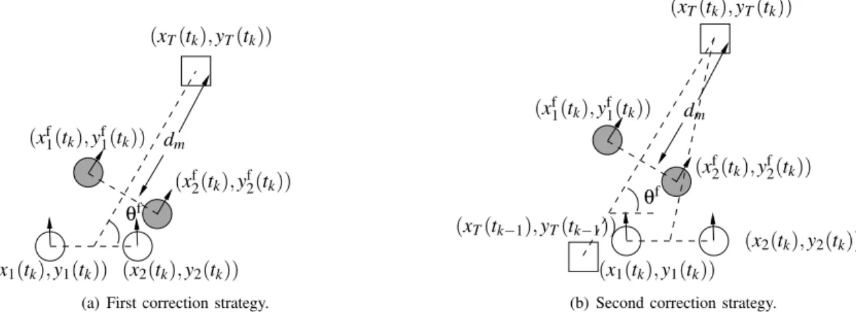
PSfrag replacements (x1(tk),y1(tk)) (x2(tk),y2(tk)) θf dm (xT(tk),yT(tk)) (xf1(tk),yf1(tk)) (xf2(tk),yf2(tk))
(a) First correction strategy.
PSfrag replacements dm θf (x1(tk),y1(tk)) (x2(tk),y2(tk)) (xT(tk−1),yT(tk−1)) (xf2(tk),yf2(tk)) (xf 1(tk),yf1(tk)) (xT(tk),yT(tk))
(b) Second correction strategy. Fig. 2. Correction strategies for the initial points at each iteration in the Formation Control level.
position attk+1is estimated. We suppose that no model of the
target is available, so a simple estimate is linear extrapolation ˆˆ xT(tk+1) =xˆT(tk) + (tk+1−tk)vˆT(tk)cos ˆθp(tk) ˆˆ yT(tk+1) =yˆT(tk) + (tk+1−tk)vˆT(tk)sin ˆθp(tk) where ˆ vT(tk) =k(xˆT(tk),yˆT(tk))t−(xˆT(tk−1),yˆT(tk−1))k k−tk−1 ˆ θT(tk) =arctanxyˆˆT(tk)−yˆT(tk−1) T(tk)−xˆT(tk−1)
The reference path provided to the low-level motion control is given by trajectories generated from the controls vi,ωi, i=1,2, wherevmandωmare continuous-time controls defined
over (tk,tk+1), such that the corresponding way point for (xm(tk+1),ym(tk+1))is reached. Ifvi,ωi,i=1,2, are constant
over an interval, they generate the following reference trajec-tories: xref i (t) =xfi(tk) +ωvi(tk) i(tk) · sin(θfi(tk) +ωi(tk)t)−sin(θfi(tk)) ¸ yrefi (t) =yfi(tk)−ωvi(tk) i(tk) · cos(θfi(tk) +ωi(tk)t)−cos(θfi(tk)) ¸
The initial reference points at each step (xif(tk),yfi(tk),θfi(tk)), i=1,2, are set to fulfill the desired formation. Those points are calculated based on the estimations of the moving target from sensors readings. Two different strategies are proposed for choosing those points. In the first, shown in Figure 2(a), we compute the new initial reference points as
θf i(tk) =arctanxyT(tk)−ym(tk) T(tk)−xm(tk) xf i(tk) =xfm(tk)±pfcos(θfi(tk)) yfi(tk) =yfm(tk)∓pfsin(θfi(tk)) PSfrag replacements (xref i (tk+1),yrefi (tk+1)) (xi(tk),yi(tk)) (xi(tk+1),yi(tk+1)) (xrefi (tk),yrefi (tk))
Fig. 3. Tracking of a trajectory generated betweentkandtk+1.
while the second one, see Figure 2(b), we use the following equations θf i(tk) =arctanxyT(tk)−yT(tk−1) T(tk)−xT(tk−1) xfi(tk) =xfm(tk)±pfcos(θfi(tk)) yf i(tk) =yfm(tk)∓pfsin(θfi(tk))
where (xm(tk),ym(tk))and(xfm(tk),yfm(tk))are defined as
µ xm(tk) ym(tk) ¶ =1 2 ·µ x1(tk) y1(tk) ¶ + µ x2(tk) y2(tk) ¶¸ µ xf m(tk) yf m(tk) ¶ = µ ˆ xT(tk) ˆ yT(tk) ¶ −dfm µ cos(θfi(tk)) sin(θfi(tk)) ¶ anddf
m and pfdepend on the desired formation.
Remark: Note that using the second strategy here proposed would require a global or inertially fixed coordinate system. In the following we use the first proposed strategy to compute the initial reference points.
B. Tracking Control
The reference trajectories (xrefi ,yrefi ),i=1,2, generated by
the high-level formation planning are tracked by the robots us-ing the virtual vehicle approach [6]. The idea is to let the mo-tion of a reference point on the reference path(xref
i (t),yrefi (t)), t ∈(tk,tk+1), be governed by a differential equation with
error feedback, see Figure 3. Consider a reference trajectory
(xref
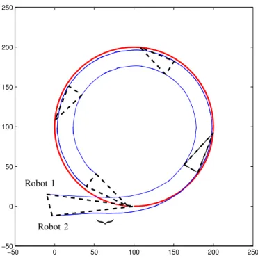
−50 0 50 100 150 200 250 −50 0 50 100 150 200 250 Robot 1 Robot 2 |{z}
Fig. 4. Robot formation tracking a target that follows a circle. The target is shown as a thick line and the robots’ trajectories as thin. Despite the errors in the initial positions of the robots, they converge to the desired formation after a few updates of the formation. Note the difference in shape between the initial formation and the following four.
the trajectories as pi(si):=xrefi (si),qi(si):=yrefi (si), i=1,2,
where ˙si is chosen as ˙ si= ce −aρv0 i q p02 i (si) +q0i2(si) where v0
i is the desired speed at which one wants roboti to
track its path (a natural choice isv0
i =vi(tk)), andaandcare
appropriate positive constants.
The low-level tracking control for roboti,i=1,2, is given
by
vi(t) =γρi(t)cos[φdi(t)−θi(t)]
ωi(t) =k[φdi(t)−θi(t)] +φ˙di(t)
where γ andkare positive tuning parameters, and ρi(t) = q (xref i (si)−xi(t))2+ (yrefi (si)−yi(t))2 φd i(t) =arctanx ref i (si)−xi(t) yref i (si)−yi(t)
Note that whenρi(t) =0, the angleφdi(t)is not well-defined.
This problem can be easily solved by re-definingφd
i when ρi
is small, see [7].
IV. SIMULATIONRESULTS
The hierarchical control algorithm developed in previous section is now evaluated through a simulated example. We let the target follow a circular trajectory and the robots have an
62 64 66 68 70 72 74 −10.05 −10 −9.95 −9.9 −9.85 −9.8 −9.75 −9.7 −9.65 −9.6
(x2ref(tk),y2ref(tk)) (x2ref(t k+1),y2ref(tk+1)) (x2(tk),y2(tk)) (x2(tk+1),y2(tk+1)) (x2f(tk+1),y2f(tk+1)) (x2f(t k),y2f(tk))
Fig. 5. A closer look to the trajectory of Robot 2 in the region marked with a big under-brace in Figure 4. The circles denote(xf
i(tk),yfi(tk)), asterisks denote (xi(tk),yi(tk))and the arrows point to(xrefi (tk),yrefi (tk)). Note that the scales of the x-axis and y-axis are different.
error in the measurement of βi with uniform distribution in (−0.02,0.02). Figure 4 shows the target as a thick line and with thin lines the trajectories of the robots. Note that despite errors in the initial positions of the robots, they converge to the desired formation after a few formation updates. The formation at the initial state and at four other locations are indicated with dashed triangles.
Figure 5 shows a closer look of one section of the trajectory of Robot 2. The zoom is taken in the beginning of the trajectory, and thus the robot is trying to converge to the high-level planner reference. The circles in Figure 5 indicate the corrected initial points(xfi(tk),yfi(tk))at each step of the
high-level planning algorithm. The stars show the final position of the tracker robots after each step, denoted(xi(tk),yi(tk)). The
arrows are pointing at the planned final points(xrefi (tk),yrefi (tk))
of the trajectory at the previous step. Figure 6 shows the evolution of target distance d2 and target angle α2 for Robot
2, corresponding to the first quarter of circle in Figure 4. The estimated and the real position of the target is shown in Figure 7.
V. EXPERIMENTALRESULTS
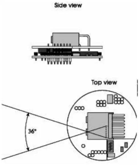
The new multi-robot algorithm presented in the paper was experimentally evaluated on a team of two Khep-era II robots [8] tracking a target LEGO Mindstorms robot. The setup is illustrated in Figure 8. Khepera II is a small self-contained wheeled robot with micro-processor and basic sensors (infra-red proximity sensors and encoders). Its diam-eter is about 70 mm, it has a precise odometry and a linear speed in the range of 0.02–1.00 m/s. Our Khepera II robots are provided with a linear video sensor, see Figure 9. It gives a directional measurement up to a distance of about 25 cm. The sensor consists of a linear light-sensitive array of 64×1 pixels, which gives an image with 256 gray levels. A major
0 2 4 6 8 10 12 14 16 18 20 0.05 0.1 0.15 0.2 0.25 0.3 0 2 4 6 8 10 12 14 16 18 20 20 40 60 80 100 120 α2 [rad] d2 [mm] t [s] t [s]
Fig. 6. Evolution ofd2andα2(Robot 2) corresponding to the first quarter of circle in Figure 4. The dashed thick line shows the desired values of(d2,α2) to fulfill the desired formation.
0 100 200 300 400 500 600 700 800 −50 0 50 100 150 200 250 0 100 200 300 400 500 600 700 800 −100 0 100 200 300 xTe(t) vs x T(t) yTe(t) vs y T(t)
measured and estimated samples
Fig. 7. Comparison of the position of the target estimated by the robots based on their sensor measurements(xe
T,yeT)(thick dashed line) vs. the real position of the target(xT,yT)(thin line).
constraint of the linear video sensor is a limited horizontal field of view of 36 degrees, i.e., the angular range is limited to αmax=π/10. For data exchange, the two robots use an
on-board radio communication system.
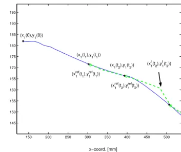
An multi-robot tracking experiment is shown in Figure 10. The target is following a smooth curve. As indicated in the figure, the desired formation is reached already after one step of the high-level planner. Figure 11 shows a closer look on how the formation is kept by the robots following the trajectories generated by the path-planner. Finally, Figure 12 presents a closer look on one of the Khepera II robots following the planned trajectory using the controller presented in Section III.
VI. CONCLUSIONS
Multi-robot estimation and tracking of a moving target was discussed in the paper. An integrated approach to sensing
Fig. 8. Two Khepera II robots tracking a LEGO Mindstorms robot.
Fig. 9. Khepera II linear vision sensor. The angular range is limited to αmax=π/10.(Illustration from [8].)
and control of two robots was presented, when each robot is equipped with a directional sensor with limited angular range. The sensor readings were fused in order to get an estimate of the targets motion. A hierarchical control strategy was developed and tested, in which high-level commands were issued to plan a series of desired formations for the robots. Low-level tracking of paths connecting waypoints defined by the formations was specified according to the recent virtual vehicle method. Ongoing work includes a systematic treatment of communication limitations in the system.
−100 0 100 200 300 400 500 600 700 800 900 −300 −200 −100 0 100 200 300 400 x−coord. [mm] y−coord. [mm]
Fig. 10. An experiment showing two Khepera II robots tracking a LEGO Mindstorms robot moving on a smooth trajectory. The lighter thick line represents the estimated trajectory of the LEGO robot, while the thicker dark lines the trajectories of the tracking robots. The evolution of the formation is shown by thick dashed triangles.
300 350 400 450 500 550 600 650 700 750 800 −50 0 50 100 150 200 y−coord. [mm] x−coord. [mm]
Fig. 11. Zoom of Figure 10 showing how the formation evolves and is kept between two steps of the high-level planner.
ACKNOWLEDGMENT
This work was supported by the European Commission through the RECSYS IST project, the Swedish Research Council and the Swedish Foundation for Strategic Research through its Centre for Autonomous Systems at the Royal Institute of Technology. 150 200 250 300 350 400 450 500 145 150 155 160 165 170 175 180 185 190 195 (x1(0),y1(0)) (x1(t1),y1(t1)) (x1(t2),y1(t2)) (x1ref(t1),y1ref(t1))
(x1ref(t 2),y1ref(t2)) (x1f(t 2),y1 f(t 2)) x−coord. [mm] y−coord. [mm]
Fig. 12. Closer look of Figure 10 showing how one of the Khepera II robots follows the trajectory derived by the formation planner. The figure presents the planned path as a dashed line and as a thin line the robot actual motion. Circles mark the desired ending points from the planned path, and asterisks mark the position of the points when the robot estimates the position of the target. Corrected points are indicated by an arrow.
REFERENCES
[1] T. Balch and R. Arkin, “Behavior-based formation control for multi-robot teams,” IEEE Transaction on Robotics and Automation, vol. 14, no. 6, pp. 926–938, 1998.
[2] B. Dunbar and R. Murray, “Model predictive control of coordinated multi-vehicle formations,” inIEEE Conference on Decision and Control, 2002. [3] P. Ögren, E. Fiorelli, and N. Leonard, “Formations with a mission: Stable coordination of vehicle group maneuvers,” inInternational Symposium on Mathematical Theory of Networks and Systems, 2002.
[4] N. Leonard and E. Fiorelli, “Virtual leaders, artificial potentials and coordinated control of groups,” in IEEE Conference on Decision and Control, 2001, pp. 2968–2973.
[5] H. G. Tanner, G. J. Pappas, and V. Kumar, “Leader-to-formation stability,” inIEEE Transactions on Robotics and Automation, 2004,(to appear). [6] M. Egerstedt, X. Hu, and A. Stotsky, “Control of mobile platforms using
a virtual vehicle approach,” IEEE Transaction on Automatic Control, vol. 46, no. 11, pp. 1777–1782, 2001.
[7] X. Hu, , D. Fuentes, and T. Gustavi, “Sensor-based navigation coordina-tion for mobile robots,” in IEEE Conference on Decision and Control, 2003.