UCLA
UCLA Electronic Theses and Dissertations
Title
Joint and Post-Selection Confidence Sets for High-Dimensional Regression Permalink https://escholarship.org/uc/item/4ww3q0pn Author Zhou, Kun Publication Date 2020 Peer reviewed|Thesis/dissertation
UNIVERSITY OF CALIFORNIA Los Angeles
Joint and Post-Selection Confidence Sets for High-Dimensional Regression
A dissertation submitted in partial satisfaction of the requirements for the degree Doctor of Philosophy in Statistics
by
Kun Zhou
c
Copyright by Kun Zhou
ABSTRACT OF THE DISSERTATION
Joint and Post-Selection Confidence Sets for High-Dimensional Regression by
Kun Zhou
Doctor of Philosophy in Statistics University of California, Los Angeles, 2020
Professor Qing Zhou, Chair
Construction of confidence sets is an important topic in statistical inference. In this disser-tation, we propose an adaptive method to construct honest confidence sets for the regression mean vector and a framework to construct confidence sets after model selection. The whole dissertation is divided into two parts.
The issue of honesty in constructing confidence sets arises in nonparametric regression. While the optimal rate in nonparametric estimation can be achieved and utilized to construct sharp confidence sets, severe degradation of confidence level often happens after estimating the degree of smoothness. Similarly, for high-dimensional regression, oracle inequalities for sparse estimators could be utilized to construct sharp confidence sets. Yet the degree of sparsity itself is unknown and needs to be estimated, which causes the honesty problem. To resolve this issue, we develop a novel method to construct honest confidence sets for sparse high-dimensional linear regression. The key idea in our construction is to separate signals into a strong and a weak group, and then construct confidence sets for each group separately. This is achieved by a projection and shrinkage approach, the latter implemented via Stein estimation and the associated Stein unbiased risk estimate. After combining the confidence sets for the two groups, our resulting confidence set is honest over the full parameter space without any sparsity constraints, while its size adapts to the optimal rate ofn−1/4 when the
true parameter is indeed sparse. Moreover, under some form of a separation assumption between the strong and weak signals, the diameter of our confidence set can achieve a faster
rate than existing methods. Through extensive numerical comparisons, we demonstrate that our method outperforms other competitors with big margins for finite samples, including oracle methods built upon the true sparsity of the underlying model.
Apart from the construction of joint confidence sets, the construction of confidence sets after model selection is essentially a different and more challenging problem, as the sampling distributions are restricted to irregular subsets, which increases the difficulty in maintaining the confidence level. To address this problem, we develop a new framework, which con-tains Bayesian interpretation and constructs credible sets conditioning on active sets of lasso estimates. This framework provides flexible choices of the prior distributions serving as reg-ularizers for the credible sets. Our preliminary research demonstrates that certain credible sets are proved to be confidence sets in the frequentist framework, yet the size of credible sets and the adaption of their diameters should be further studied. Lastly, we seek the pos-sibility to generalize this framework into a large amount of generalized linear models and into confidence sets conditioning on block lasso estimates.
The dissertation of Kun Zhou is approved.
Yingnian Wu Hongquan Xu
Jingyi Li
Qing Zhou, Committee Chair
University of California, Los Angeles 2020
This dissertation work is specially dedicated to my mother whose words of encouragement inspire me all the time.
TABLE OF CONTENTS
1 Introduction . . . 1
1.1 Inference on the mean vector . . . 2
1.2 Inference on the coefficient vector . . . 5
1.3 Inference on the individual coefficient . . . 7
1.4 Post-selection inference . . . 10
1.5 Outline and overview . . . 12
2 A Two-Step Stein Method . . . 14
2.1 Introduction . . . 15
2.2 Method of construction . . . 17
2.3 Adaptation of the diameter . . . 20
2.4 Multiple candidate sets . . . 23
2.5 Algorithm and implementation . . . 26
2.6 Estimated noise variance . . . 28
2.7 Proofs . . . 30
3 Empirical Study: Two-Step Stein Method v.s. Other Competitors . . . 39
3.1 Competing methods . . . 39
3.1.1 Lasso prediction error . . . 39
3.1.2 Another adaptive method . . . 40
3.1.3 An oracle lasso method . . . 42
3.1.4 A two-step lasso method . . . 43
3.2 Numerical results . . . 46
3.2.2 Results on the two-step Stein method . . . 48
3.2.3 Comparison with the two-step lasso method . . . 51
3.2.4 Dense signal settings . . . 54
3.2.5 Estimated error variance . . . 57
3.2.6 Normality and homogeneity assumptions . . . 59
3.3 Real data analysis . . . 62
4 Post-Selection Inference with Estimator Augmentation . . . 66
4.1 Estimator augmentation . . . 67
4.2 Posterior distribution and inference after model selection . . . 70
4.2.1 Conditional posterior distribution . . . 71
4.2.2 Construction of credible sets . . . 74
4.3 Estimator augmentation in GLMs . . . 78
4.3.1 Decision-theoretic framework . . . 79
4.3.2 Exponential families . . . 81
4.3.3 Low-dimensional setting . . . 83
4.3.4 High-dimensional setting . . . 85
4.4 Post-selection inference with blocked lasso . . . 85
LIST OF FIGURES
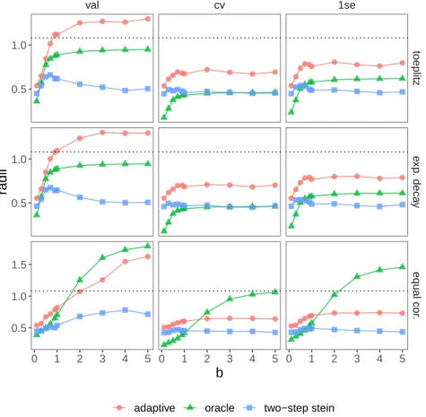
3.1 Geometric average radius against b under the first way of generating β. Each panel reports the results for one type of design (row) and one way of choosing λ
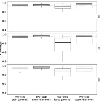
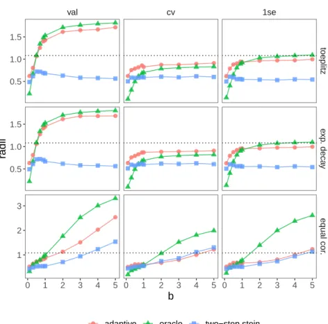
(column), where the dashed line indicates the naive χ2 radius. . . 49 3.2 Average radius ¯r against b in the second scenario of generating β. . . 50 3.3 Box plots of coverage rates for each choice of λ, pooling data from three designs.
The dashed lines indicate the desired confidence level of 95%. . . 51 3.4 Average radius ¯r against b in the first scenario of generating β. . . 52 3.5 Box plots of coverage rates for each choice of λ. The dashed lines indicate the
desired confidence level of 95%. . . 53 3.6 Comparison results under dense signal settings. (a) and (b) Geometric average
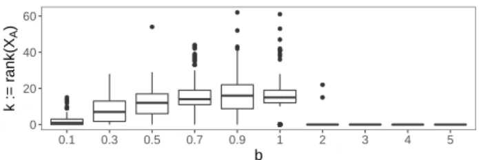
radius against b. (c) and (d) Box plots of the coverage rates. . . 55 3.7 The box plot of k across data sets for each value of b . . . 56 3.8 Average radius ¯r against b with estimated error variance ˆσ2. . . . 58
3.9 Box plots of coverage rates for each choice of λ with estimated ˆσ2. The dashed lines indicate the desired confidence level of 95%. Outliers below 0.75 are trun-cated. . . 59 3.10 (Upper) Average radius ¯r againstb and (lower) box-plots of coverage rates of all
settings under t-distributions or heterogeneous error variance. The dashed lines in the four top panels indicate the average naive χ2 radius. The dashed lines in the box-plots indicate the nominal coverage level of 95%. . . 61 3.11 Hierarchical clustering of gene expression vectors among 72 individuals. . . 62
LIST OF TABLES
3.1 Comparison between the two-step Stein method and the adaptive method over 400 data sets based on the riboflavin data set. . . 64 3.2 Confidence sets constructed on the riboflavin data set. . . 65
ACKNOWLEDGMENTS
I would like to express my sincere gratitude to my supervisor Qing Zhou for his consistent support and guidance throughout my research. I benefit from every meeting, discussion and question and am grateful for his patience, motivation, enthusiasm, and immense knowledge.
VITA
2011–2015 B.S., Department of Mathematics, Zhejiang University
2015–2020 Teaching Assistant and Graduate Student Researcher, Department of Statistics, University of California, Los Angeles
CHAPTER 1
Introduction
Statistical inference is one of the most important fields in the current research. Particularly, high-dimensional inference has been receiving significant attention, since there is a growing demand for methodologies and theories when data is insufficient compared to the number of parameters in models. For example, in biology, especially genetics, researchers want to screen out a small group of genes associated with one specific trait among millions of genes, while the number of subjects is limited. More examples include finance, social networking, online advertising and the list goes on. To broaden the scope of high-dimensional inference, this dissertation aims at providing a novel adaptive method to construct confidence sets for the mean vector in regression models and a new framework of constructing confidence sets after model selection. Before formally presenting our ideas, we review three adaptive methods for regression models, which correspond to three topics on statistical inference: the inference on the mean vector, the inference on the coefficient vector and the inference on the individual coefficient. Besides, we review Stein estimation (Li, 1989), on which our method is based, and a simulation-based method for post-selection inference.
The Stein estimation and the adaptive method for the mean vector are discussed in Section 1.1. The rest of two adaptive methods are discussed in Section 1.2 and Section 1.3, respectively. The method for post-selection inference is discussed in Section 1.4. Lastly, we describe the outline of this dissertation in Section 1.5.
1.1
Inference on the mean vector
Our problem is directly related to the construction of confidence sets in nonparametric regression, for which a line of work has laid down important theoretic foundations and provided methods of construction (Li, 1989; Beran and D¨umbgen, 1998; Baraud, 2004; Robins and van der Vaart, 2006; Cai and Low, 2006). Beran and D¨umbgen (1998) mentioned that the problem of recovering a signal from observation of the signal plus noise may be formulated as inference of the mean vector, which justifies the practical importance of inference on the mean vector.
Li (1989) provided a fundamental study for this problem. The author considered the nonparametric statistical model
y=µ+ε,
where y ∈ Rn is the observed vector, µ ∈
Rn is the unknown mean vector and ε ∼ Nn(0, σ2In). Their aim is to construct an asymptotic confidence setCb=Cbnof small diameter
for µ, which achieves honesty in the sense that, for any significance level α∈(0,1), lim inf
n→0 µinf∈RnP{µ∈Cb} ≥1−α. (1.1)
Note that (1.1) means that the confidence set should achieve the nominal significance level for anyµ∈Rn. A naive confidence set can be constructed by{µ∈
Rn: 1nkµ−yk2 ≤ σ
2
nχ
2
n,α},
where χ2n,α denotes the (1−α)-quantile of χ2-distribution with n degrees of freedom. It is easy to verify such a naive confidence set satisfies honesty property. However, the normalized radius σn2χ2n,α is of the order of 1, indicating the diameter never converges, and thus it is of limited interest. The author further proved that any honest confidence set satisfying (1.1) cannot have a diameter converging at a rate faster than n−1/4.
The achievability of this optimal raten−1/4 is demonstrated by a simplified Stein estimate
Nn(µ, σ2In) and Tn ∈Rn×n, let Rn=In−Tn,and define ˆ µ(y; ˜µ) =y− σ 2tr(R n) kRnyk2 Rny, (1.2) ˆ L(y; ˜µ) = 1− σ 2(tr(R n)) 2 nkRnyk2 , (1.3)
where ˆµ(y; ˜µ) is the Stein estimate associated with the initial estimate ˜µ and σ2Lˆ(y; ˜µ) is
the Stein unbiased risk estimate (SURE). Li (1989) proved the uniform consistency of ˆL.
Lemma 1 (Theorem 3.1 in Li (1989)). Assume that y ∼ Nn(µ, σ2In). For any α ∈ (0,1),
there exists a constant cs(α)>0 such that
lim inf n→∞ µinf∈RnPµ n σ 2ˆ L−n−1kµˆ−µk2 ≤cs(α)σ 2 n−1/2 o ≥1−α, (1.4)
where µˆ and Lˆ are defined in (1.2) and (1.3).
By Lemma 1, we let ˆµ be the center and σ2Lˆ+c
s(α)n−1/2 be the radius to construct a
confidence set in the form of {µ: kµ−µˆk2 ≤σ2Lˆ+c
s(α)n−1/2}. It follows from (1.4) that
such a confidence set satisfies (1.1). The Stein method can achieve the optimal rate of n−1/4
if ˜µ is close to µ in the sense of `2-norm. That is, y is shrunk to the subspace that µ lies in. Baraud (2004) proposed another method with multiple hypotheses, which increases the chance of adaption at the optimal rate.
Here, we introduce an adaptive method (Robins and van der Vaart, 2006), which con-structs an honest confidence set for a Hilbert space-valued parameter including the mean vector in Rn. The authors provided five different models as examples — a model with
reg-ular parameters, a finite sequence model, an infinite sequence model, a density estimator and random regression — to illustrate the wide application of their method. Particularly, under a finite sequence model, the observation is a vector following the n-dimensional nor-mal distribution with a mean vector θ = θ(n) = (θ1, θ2, . . . , θn)T and a covariance matrix
σ2
nIn. The variance σ
2 is known and the parameter θ belongs to a subset Θ of
Rn, where Θ is possibly equal to Rn. They justified that the confidence set by their method is honest over the parameter space Θ and its diameter adapts to a subset of Θ to achieve the optimal diameter rate n−1/4.
Their method is based on sample splitting. Suppose an initial estimator ˆθ = ˆθ(n) inde-pendent of y is given. Their confidence set is connected with an estimator Rn=Rn(ˆθ, y) of
the squared norm kθ−θˆk2 such that
lim n→∞θinf∈ΘPθ n Rn(ˆθ)− kθ−θˆk2 ≥ −zατˆn,θ|θˆ o ≥1−α, (1.5)
where ˆτn,θ is a “scale estimator” and zα is a quantile. Following from (1.5), one can derive
an honest confidence set
b Cn = θ ∈Θ :kθ−θˆk ≤ q zατˆn,θ+Rn(θ) . (1.6)
Note that Cb may not be a ball as the right hand side of (1.6) is also a function of ˆθ. Tne inequality (1.5) demonstrates that the confidence set (1.6) essentially depends on a good estimatorRnto achieve the adaptive diameter, while being honesty over Θ. The authors used
the construction by Laurent (1996, 1997) forRn. This construction is based on estimating the
squared norm of the projection ofθ−θˆbykΠkθ−Πkθˆk2, where Πkθ = (θ1, . . . , θk,0, . . . ,0),
and minimizing the total effect of the resulting bias and the variance of the estimator. The bias can bounded above by a multiple of
Bk2:= sup
θ∈Θ
kθ−Πkθk2. (1.7)
Note that when Θ =Rn, Bk2 =∞for any k < n. The variance is of the order of
ˆ τk,n,θ:= 2σ4k n2 + 4σ2kΠkθ−Πkθˆk2 n . (1.8)
Let|Cb| denote the diameter of the confidence set. Combining (1.7) and (1.8) together, they showed that Cb is honest over Θ with its diameter
|Cb|=Op( σk1/4 √ n +Bk+kθ− ˆ θk), (1.9)
where k can be chosen by an optimal value to minimize the order. For any Rn which is of
the same order askΠkθ−Πkθˆk2, the result in (1.9) is still valid. One can see from (1.9) that
kθ−θˆkis the key to improve the diameter. If ˆθ performs well for a subset of Θ,k1/4/√n and
Bk dominate in (1.9). When Θ =Rn, |Cb| in (1.9) is reduced to |Cb|=Op(σn−1/4+kθ−θˆk) verifying n−1/4 is the optimal rate for the honest confidence set over Rn.
Further, under the aforementioned finite sequence model, they derived the estimator of kθ−θˆk2, Rk,n(θ) = k X i=1 (Xi−θˆi)2− kσ2 n , (1.10)
and the associated scale estimator,
ˆ τk,n,θ2 = 2kσ 4 n2 + 4σ2 n k X i=1 (θi−θˆi)2. (1.11)
With such a choice, zα in (1.5) is the (1−α)-quantile of the standard normal distribution.
Later, we will compare our method against this adaptive method by Robins and van der Vaart (2006).
1.2
Inference on the coefficient vector
Consider a linear model
y=Xβ+ε, (1.12)
where y ∈ Rn, X ∈
Rn×p, β ∈ Rp and ε ∼ N(0, σ2In). The inference on β is of great
interest for various purposes: model selection, point estimation, hypothesis testing, etc. Carpentier (2015) proposed a method to construct a confidence set for β, which adapts to the unknown sparsity, under the assumption of a separation between large and small coefficients. Recently, Ewald and Schneider (2018) provided an exact formula to compute a lower bound of the coverage rate of a confidence set centered at the lasso, over the entire parameter space for any significance level α∈(0,1), and vice versa; however, low dimension (p < n) is a vital condition in their proof, making it impossible to generalize their idea to the high-dimensional problem that we are studying. Besides, Cai and Guo (2020) considered semi-supervised inference for explained variance, i.e.,βTΣβ, where Σ is the covariance matrix
of a random design matrix, and then applied it to construct a confidence set for β. We present the important finding in Nickl and van de Geer (2013) in the rest of this section. In Section 1.1, we have seen that as the space ofµ=Xβ isRn, the confidence set for µcannot
maintain the honesty with |Cb| = o(n−1/4). Nickl and van de Geer (2013) showed that this conclusion is also valid to the confidence set for β and the adaption to sparsity at a faster rate o(n−1/4) can only happen when a small region is removed from the parameter space of β.
Denote by B0(k) ={β ∈Rp :kβk0 ≤k} the subset of Rp, where the number of nonzero
coefficients is no more than k. The authors studied a sparse linear model (1.12) in the sense that β ∈ B0(k1) and k1 = k1(a1) ∼ p1−a1 for 0 < a1 < 1. Here, a1 ∈ (0,12] is considered
as a moderately sparse case and a1 ∈ (12,1) is considered as a highly sparse case. Under
proper conditions andk1 =o(n/logp), they proved that there exists a confidence set Cb that is honesty over B0(k1) in the sense of
lim inf n→∞ β∈infB0(k1)Pβ n β∈Cb o ≥1−α
with any given significance level. Moreover, for any k ≤ k1 and β ∈ B0(k), its diameter satisfies
|Cb|2 =Op(
k
n logp+n
−1/2). (1.13)
In high-dimensional inference, the equation (1.13) indicates that the construction of confi-dence sets is essentially a different problem from the estimation of risk bound, where a sparse adaptive estimator ˆβ = ˆβ(X, y) can satisfy
kβˆ−βk2
. k
n logp
up to a multiplicative constant in high probability.
Their next interest is what kind of critical region could be removed from B0(k1) to
encourage adaption to sparsity at any rate o(n−1/4). Let B0(k0) be a subset of B0(k1) with k0 ∼p1−a0. Clearly, k0 < k1 and a0 > a1. Then, remove those β ∈B0(k1) that are close in `2-distance to B0(k0) to get
˜
B0(k1, ρ) ={β ∈B0(k1) :kβ−B0(k0)k ≥ρ},
where ρ=ρn,p is a separation sequence and kβ−Bk:= infb∈Bkβ−bk for any B ⊆Rp. The
setCbn,p for β satisfying a weaker honesty property lim inf n→∞ β∈Binf(ρn,p)P β n β ∈Cbn,p o ≥1−α (1.14)
for anyα∈(0,1). Besides, its diameter satisfies that, for some constantL >0 andα0 ∈(0,1), lim sup n→0 sup β∈B0(k0) Pβ |Cbn,p|2 > L k0 n logp ≤α0 (1.15) and lim sup n→0 sup β∈B0˜ (k1,ρn,p)P β |Cbn,p|2 > L k1 n logp ≤α0. (1.16)
Assuming certain conditions as well as k0 =o(
√
n/logp) and k1 =o(n/logp), they proved
that a confidence set satisfying (1.14), (1.15) and (1.16) exists if and only if ρn,p & n−1/4,
where & denotes greater than up to a multiplicative constant. In a moderately sparse case that 0 < a1 ≤ 1/2 < a0 ≤ 1, ρn,p attains the rate of n−1/4. On the other hand, in a
highly spare case that 12 < a1 < a0 ≤ 1, the rate of ρn,p can be potentially relaxed from
n−1/4 to min{k1
n logp, n
−1/4}. This conclusion affirms that (1.13) cannot be improved if the
confidence sets are honest over all B0(k1). One may question if the ρ-separation condition
can be avoided at the cost of a mild penalty added to the adaption rate in (1.15). The authors remarked that such a penalty does not alter the necessity of ρn,p & n−1/4 by their
proof.
1.3
Inference on the individual coefficient
Under the linear model (1.12), the construction of confidence sets for µ = Xβ or β is different in nature from the construction of confidence intervals for an individual βj or a
low-dimensional projection of β. For the latter, the optimal rate of an interval length can be n−1/2 when β is sufficiently sparse (Schneider, 2016; Cai and Guo, 2017), such as the intervals constructed by de-biased lasso methods (Zhang and Zhang, 2014; van de Geer et al., 2014; Javanmard and Montanari, 2014). Although simultaneous inference methods have been proposed based on bootstrapping de-biased lasso estimates (Zhang and Cheng,
2017; Dezeure et al., 2017), these methods are shown to achieve the desired coverage only for extremely sparse β such that kβk0 = o(
p
n/(logp)3), which severely limits their practical
application. We introduce another adaptive method proposed by Cai and Guo (2017), which is based on the convergence rates of the minimax expected length for confidence intervals.
Specifically, the authors considered constructing a confidence interval for a linear func-tional T(β) =ξTβ, where ξ ∈Rp is named as the loading vector. Let k denote the sparsity
level, i.e., kβk0 ≤ k. Based on the sparsity of ξ, they define a sparse loading regime where
only a part ofξi is nonzero, say kξk0 .k, and a dense loading regime where |ξ| k. A
typ-ical example for sparse loading regime is T(β) = βi and a typical example for dense loading
regime is T(β) = Pp
i=1βi. We first introduce their “minimax expected length” framework.
They assume the Gaussian design that all rows of Xi. i.i.d.
∼ Np(0,Σ), and Σ and σ are both
unknown. Denote as θ= (β,Σ−1, σ) the tuple of all parameters. Given the significance level
α∈(0,1), a parameter space Θ⊆Rp of β and a linear functional T(β), letI
α(Θ, T) be the
set of all honesty confidence intervals for T(β) over Θ, namely, Iα(Θ, T) = CIα(T, Z) = [l(Z), u(Z)] : inf θ∈ΘPθ{l(Z)≤T(β)≤u(Z)} ≥1−α ,
whereZ = (X, y) is the observed data,l(Z) is the lower bound andu(Z) is the upper bound. For any honesty confidence interval CIα(T, Z) ∈ Iα(Θ, T), define the maximum expected
length over a parameter space Θ as
L(CIα(T, Z),Θ, T) = sup θ∈ΘE
θL(CIα(T, Z)),
where L(CIα(T, Z)) = u(Z) −l(Z) is the length of that confidence interval. Given two
parameter spaces Θ1 ⊆Θ, define
L∗α(Θ1,Θ, T) := inf
CIα(T ,Z)∈Iα(Θ,T)
L(CIα(T, Z),Θ1, T).
Essentially, Iα(Θ, T) is the infimum of the maximum length of confidence intervals over the
subspace Θ1, when these confidence intervals are honest over Θ with α significance level. If
Θ1 = Θ,L∗α(Θ, T) = L
∗
α(Θ,Θ, T) is exactly the minimax expected length of honest confidence
should satisfy
L(CIα(T, Z),Θ1, T)L∗α(Θ1, T), L(CIα(T, Z),Θ, T)L∗α(Θ, T).
In other words, the length of this CIα(T, Z) should be of the order of the optimal length
simultaneously over Θ1 and Θ, while CIα(T, Z) maintains the honesty over Θ. As a
conse-quence, if L∗α(Θ1,Θ, T)L∗α(Θ1, T), the sparse adaption to Θ1 from Θ is unfeasible.
Letk andk1 respectively denote the sparsity of Θ and Θ1. For the sparse loading regime,
the authors proved that with the condition k1 < k ≤min{pγ,lognp} for γ ∈(0,1),
L∗α(Θ, T) kξk2 1 √ n +k logp n , (1.17) L∗α(Θ1,Θ, T)≥c1kξk2 1 √ n +k logp n σ, (1.18)
where c1 > 0 is a constant. It can bee seen from (1.17) that the length of the honest
confidence interval cannot adapt at o(n−1/2). The inequality (1.18) indicates that when
√
n
logp k . n
logp and k1 k, there does not exist an honest confidence interval that adapts
to Θ1, since L∗α(Θ1,Θ, T)L∗α(Θ, T) kξk2k logp n L ∗ α(Θ1, T).
Therefore, the adaption can only be achieved in the ultra-spare case k .
√
n
logp, while the
optimal rate n−1/2 does not depend on sparsity in this case. For the dense loading regime,
they proved that
L∗α(Θ, T) kξk∞k r logp n , (1.19) L∗α(Θ1,Θ, T)≥c1kξk∞k r logp n σ, (1.20)
where c1 >0 is a constant. It follows from (1.19) and (1.20) that
L∗α(Θ1,Θ, T)&kξk∞k r logp n L ∗ α(Θ1, T),
which means that the the adaption in the dense loading regime is impossible. Lastly, they studied whether the prior knowledge Σ = In and σ = σ0 can improve the result. For the
sparse loading regime, the minimax expected length is improved and becomes
L∗α(Θ, T) k√ξk2
n
so that an adaptive honest confidence interval for T(β) is possible over Θ with k=O(lognp), while for the dense loading regime, the prior knowledge cannot improve the minimax expected length.
1.4
Post-selection inference
Post-selection inference is a topic different from the previous topics and attracts increasing interest in recent years. (Berk et al., 2013; Lee et al., 2016; Tibshirani et al., 2016; Tian and Taylor, 2017; Taylor and Tibshirani, 2018; Liu et al., 2018).
Min and Zhou (2019) developed a novel method to construct a confidence set after lasso variable selection. Their method takes advantages of the closed-form sampling density condi-tioning on a lasso active set (Zhou, 2014) and a randomization step. Together with a carefully developed Markov chian Monte Carlo (MCMC) algorithm, they empirically showed that the confidence set constructed by their method can achieve the desired coverage rate with its di-ameter substantially smaller than other state-of-the-art methods. We summarize their work in the rest of the section. Consider (1.12) with a fixed design matrix X. The parameter of interest is
ν:=XA+µ0 = argmin
β∈R|A|
kµ0−XAβk2, (1.21)
where µ0 =Xβ, namely, the projection of µ0 onto the column space spanned by XA.
Infer-ence on ν becomes more challenging when the selection of A is also based on the same data set (X, y), because the distribution of ν essentially conditions on the model selection event. In their method, the selection step is achieved by the lasso estimator, namely,A = supp( ˆβ). The primary goal is to construct a marginal confidence interval for νj conditioning on
A =A with a desired coverage. One possible direction is to construct a confidence interval from [{XA+(y∗−µ˜)}j|A(y∗) = A] where ˜µis an estimate ofµandy∗ denotes a sample drawn
from an estimated distribution ofy (e.g., y∗ ∼ Nn(˜µ, σ2In)). However, it is unrecommended
due to the lack of theories to support that [XA+(y∗−µ˜)|A(y∗) =A] is a consistent estimator for [XA+(y−µ0)|A(y) = A]. Therefore, the coverage rates of this raw method could drop
with a poor choice of ˜µ. We can theoretically develop a confidence interval for νj without
knowing the true value ofµ0. Let a setC ⊆Rn satisfyµ0 ∈C and qj,α(µ) be theα-quantile
of [{XA+(y∗ −µ)}j|A(y∗) =A] where y∗ ∼ Nn(µ, σ2In). For any α <1/2, define
qj,α∗ (C) = min
µ∈C qj,α(µ), q
∗
j,1−α(C) = max
µ∈C qj,1−α(µ).
If Cb is a (1−α/2) confidence set for µ0, then
P νj ∈[ˆνj −qj,α/∗ 4(Cb),νˆj−qj,∗1−α/4(Cb)] A(y) = A ≥1−α, (1.22)
where ˆνj = [XA+y]j is the center of this confidence interval. Determining its length by
the worst scenarios over all µ ∈ Cb, the confidence interval [ˆνj −qj,α/∗ 4(Cb),νˆj −qj,∗1−α/4(Cb)] maintains the significance level. Inspired by this conservative method, they proposed a three-step simulation-based algorithm to trade off incorporating more variation than single estimate ˜µ versus controlling the interval length:
1. Draw ˜u(k) uniformly from a (1 − α) confidence set
b
C for µ0. Denote the uniform
distribution over Cb as U(Cb). When n is large, one can sample from the boundary of b
C,U(∂Cb), as most points in Cb are close to the boundary. 2. For each ˜u(k), draw {y∗
k,i}i from [y∗|A(y∗) = A], the density of which is derived by
estimator augmentation (Zhou, 2014) with a point estimate ˜u(k) in place of the true
µ0.
3. Construct a confidence interval for νj based on the quantiles of {XA+(y
∗
k,i−µˆ)j}, where
ˆ
µis some estimate of µ0.
The randomization of the plug-in ˜µ(k) has a Bayesian interpretation. Regard U(Cb) as a posterior distribution for µ0 and let the density be p(µ0|y). Then samples are drawn from
the posterior distribution of y∗ conditioning on A, i.e.,
p(y∗|A(y∗) =A, y) = Z
Further, the algorithm can be generalized to learn the joint distribution kH(XA+y∗−XA+µˆ)kδ A(y∗) = A , (1.23) where H ∈ Rm×|A|, m ≤ |A| and k.k
δ is the`δ-norm, and then a (1−α) confidence set for
Hν can be
{η ∈Rm :kη−Hνˆk
δ ≤q}
where q is the (1−α)-quantile of the distribution in (1.23). One typical choice is to let
H =Im×m and δ = 2 to do the inference onν in (1.21).
1.5
Outline and overview
In this dissertation, we propose an adaptive method to construct a confidence set and a new framework for post-selection inference. Remaining chapters of this dissertation are structured as follows:
• Chapter 2 develops our two-step Stein method in details, including its theoretical properties and algorithmic implementation.
• Chapter 3 presents three alternative methods to construct confidence sets. A various amount of simulations and real-data analysis are conducted to illustrate the effective-ness of our two-step Stein method.
• Chapter 4 establishes a new framework for constructing confidence sets after model selection and includes a preliminary study of its theoretical properties.
• Chapter 5 concludes this dissertation with further discussions and future work.
Notations used throughout the dissertation are defined here. We denote by Pβ the
dis-tribution of [y | X] and Eβ the corresponding expectations, where the subscript β may be
dropped when its meaning is clear from the context. Denote by [p] the index set {1, . . . , p} and by|A|the size of a setA⊆[p]. Writean= Ω(bn) ifbn =O(an) andanbnifan =O(bn)
andbn=O(an). We use Ωp(.) and p if the above statements hold in probability. For a
vec-torv = (vj)1:m, letvA= (vj)j∈Abe the restriction ofv to the components inA. For a matrix
M = [M1 |. . .|Mm], where Mj is the jth column, denote by MA= (Mj)j∈A the submatrix
consisting of columns in A. Similarly, define MBA = (Mij)i∈B,j∈A and MB· = (Mij)i∈B. For
a, b∈Rn, ha, bi:=aTb is the inner product. Definea∨b:= max{a, b} and a∧b:= min{a, b}
CHAPTER 2
A Two-Step Stein Method
Consider high-dimensional linear regression
y=Xβ+ε, (2.1)
where y∈Rn, X = [X
1| · · · |Xp]∈Rn×p, β ∈Rp, ε∼ Nn(0, σ2In) and p > n. While there is
a rich body of research on parameter estimation under this model concerning signal sparsity (e.g. Bickel et al. (2009); Zhang and Huang (2008); Negahban et al. (2012)), how to construct confidence sets remains elusive. In this work, we focus on confidence sets for the mean
µ = Xβ with the following two properties: First, the confidence set Cb is (asymptotically) honest over all possible parameters. That is, for a given confidence level 1−α,
lim inf n→∞ βinf∈RpPβ n Xβ ∈Cb o ≥1−α, (2.2)
where Pβ is taken with respect to the distribution of y ∼ Nn(Xβ, σ2In), regarding X as
fixed. Second, the diameter of Cb is able to adapt to the sparsity and the strength of β. In practical applications, sparsity assumptions are very hard to verify, and for many data sets they are at most a good approximation. The first property guarantees that our confidence sets reach the nominal coverage without imposing any sparsity assumption, while the second property allows us to leverage sparse estimation when β is indeed sparse.
Throughout the chapter, we always assume model (2.1) with ε ∼ Nn(0, σ2In) unless
otherwise noted. The remainder of this chapter is organized as follows. We introduce more detailed background, demonstrate our motivation and formulate the problem in Section 2.1. Section 2.2 develops our two-step Stein method. Section 2.3 studies the size of the confidence sets by our method. We provide a data-driven selection of the candidate set in Section 2.4 and develop the implementable algorithm in Section 2.5. Section 2.6 considers theoretical
properties when estimated error variance is plugged in. Finally, all proofs are included in Section 2.7.
2.1
Introduction
Despite notable advances of many developed methods in Section 1.1, lack of numerical sup-port casts doubt on the merit of borrowing these nonparametric regression methods directly for sparse regression. Taking the adaptive method based on sample splitting in Robins and van der Vaart (2006) in Section 1.1 as an example, an honest confidence set for µ can be constructed as Cba = {µ ∈ Rn : n−1/2kµ−Xβˆk ≤ rn}, where Xβˆ is an initial estimate independent ofy, and its (normalized) diameter |Cba|:= 2rn=Op(n−1/4+n−1/2kXβˆ−Xβk).
A common choice for ˆβ under model (2.1) for p > n is a sparse estimator, such as the lasso (Tibshirani, 1996) or `0-penalized least-squares estimator. With high probability, the
prediction loss of the lasso estimator typically satisfies 1
nkX
ˆ
β−Xβk2 ≤cslogp
n (2.3)
for some c > 0, uniformly for all β ∈ B(s) := {v ∈Rp : kvk
0 ≤ s}; see for example Bickel
et al. (2009). Under this choice, the diameter |Cba| is of the order |Cba|=Op
n−1/4+pslogp/n (2.4)
for all β ∈ B(s). For a precise statement, see Theorem 8 below. This method has nice theoretical properties when s = o(n/logp). But even for moderately sparse signals with
s/n → δ ∈ (0,1), the bound on the right side of (2.4) approaches ∞ as p > n → ∞ and thus offers little insight into the performance of the confidence set. The upper bound (2.3) also critically depends on the regularization parameter used for the initial estimate ˆβ. In fact, our numerical results show that, for finite samples with (s, n, p) = (10,200,800), this confidence set can be worse than a naive χ2 region {µ : ky−µk2 ≤ σ2χ2
n,α}, where χ2n,α
denotes the (1−α)-quantile of the χ2 distribution with n degrees of freedom. A similar issue occurs in the related but different problem of constructing confidence sets for β. Nickl and van de Geer (2013) in Section 1.2 have shown that one can construct a confidence set
for β that is honest over B(k1) for k1 = o(n/logp), and for any s ≤k1, the diameter is on
the same order as that in (2.4) for any β ∈B(s). Compared to the unrestricted honesty in (2.2) over the entire space Rp, the restriction on the honesty region to B(k
1) also reflects
the challenge faced in the construction of confidence sets when p > n.
The construction of confidence sets is fundamentally different from the problem of in-ferring error bounds for a sparse estimator (Nickl and van de Geer, 2013). It is seen from (2.4) that no matter how sparse the true β is, the diameter of Cba cannot converge at a rate faster than n−1/4. Indeed, results in Li (1989) imply that, for the linear model (2.1) with
p ≥ n, the diameter of an honest confidence set for µ, in the sense of (2.2), cannot adapt at any rate o(n−1/4). This is in sharp contrast to error bounds for a sparse estimator, such as that in (2.3), which can decay at a much faster rate when β is sufficiently sparse. It is not desired to construct confidence sets directly from error bounds like (2.3) even we only require honesty for β ∈ B(k1) with a given k1 = o(n/logp), because its diameter, on the
order of pk1logp/n, cannot adapt to any sparserβ ∈B(s) for s < k1.
Motivated by these challenges, we propose a new two-step method to construct a confi-dence set forµ=Xβ, allowing the dimension pn in (2.1). The basic idea of our method is to estimate the radius of the confidence set separately for strong and weak signals defined by the magnitude of|βj|. Using a sparse estimate, such as the lasso, one can recover the set
A of large |βj| accurately and expect a small radius for a confidence ball forµA, the
projec-tion of µ onto the subspace spanned by Xj, j ∈A. By construction, (µ−µA) is composed
of weak signals. Thus, in the second step, we shrink our estimate of this part towards zero by Stein’s method and construct a confidence set with Stein’s unbiased risk estimate (Stein, 1981). Combining the inferential advantages of sparse estimators and Stein estimators, our method overcomes many of the aforementioned difficulties. First, our confidence set is honest for all β ∈ Rp, and its diameter is well under control for all possible values of β including
the dense case. Second, by using elastic radii our confidence set, an ellipsoid in general, can adapt to signal strength and sparsity. The radius for strong signals adapts to the sparsity of the underlying model via sparse estimation or model selection, while the radius for weak signals adapts according to the degree of shrinkage of the Stein estimate. Without any signal
strength assumption, the diameter of our confidence set isOp(n−1/4+
p
slogp/n), the same as (2.4), for β∈B(s). It may further reduce toOp(n−1/4+
p
s/n) under an assumption on the separability between the strong and the weak signals, which shrinks to the optimal rate
n−1/4 when the signal sparsity s =O(√n), as opposed to s=O(√n/logp) in (2.4). Third, in addition to proving the optimal rates like many existing works, we made a lot of efforts in approximating all involved constants in our method, making it practical in real data analysis. We provide a data-driven selection of the setAfrom multiple candidates, which protects our method from a bad choice and thus makes it very robust. We demonstrate with extensive numerical results that our method can construct much smaller confidence sets than other competing methods, including the adaptive method (Robins and van der Vaart, 2006) dis-cussed above and oracle approaches making use of thetrue sparsity of β (the oracle). These results highlight the practical usefulness of our method.
2.2
Method of construction
Dividingβinto strong and weak signals, our method constructs a confidence setCb(y) with an ellipsoid shape forXβ that is honest as defined in (2.2). Note that under a high-dimensional asymptotic framework, all variablesX =X(n),y =y(n),β =β(n) ands=sn depend on n
as p=pn n → ∞, while X(n) is regarded as a fixed design matrix for each n. We often
suppress the dependence on n to simplify the notation.
Now, consider the linear model (2.1) and letµ=Xβ. Given a pre-constructed candidate setA =An ⊆[p], independent of (X, y), define
µA=PAµ, µ⊥ =PA⊥µ= (In−PA)µ,
where PA is the orthogonal projection from Rn onto span(XA) and PA⊥ is the projection to
the orthogonal complement. A good candidate setAis supposed to include all strong signals, say A={j :|βj|> τ}. With such a choice, kµ⊥k will be small. Typically, we split our data
set into two halves, (X, y) and (X0, y0), and apply a model selection method on (X0, y0) to construct the set A. See Section 2.3 for more detailed discussion.
We estimate µA and µ⊥, respectively, by ˆµA and ˆµ⊥, compute radii rA and r⊥, and
construct a (1−α) confidence set Cb for µ in the form of
b C = µ∈Rn: kPAµ−µˆAk2 nr2 A + kP ⊥ Aµ−µˆ⊥k2 nr2 ⊥ ≤1 . (2.5)
Note thatCbis an ellipsoid inRn, whererA=rA(α) andr⊥ =r⊥(α) correspond to the major
and minor axes, respectively. Our method consists of a projection and a shrinkage step:
Step 1: Projection. Let ˆµA =PAy and k = rank(XA)≤ |A|. Since A is independent of
(y, X), we have
kˆµA−µAk2 =kPAεk2 |A∼σ2χ2k. (2.6)
Thus, we choose
r2A=c1˜rA2 =c1σ2χ2k,α/2/n, (2.7)
whereχ2
k,α/2 is the (1−α/2)-quantile of the χ 2
k distribution andc1 >1 is a constant, so that
P k PAµ−µˆAk2 nr2A ≤1/c1 = 1−α/2. (2.8)
Step 2: Shrinkage. Let y⊥ =PA⊥y. As mentioned above, under a good choice of A that
contains strong signals, kµ⊥k is expected to be small. Therefore, we shrink y⊥ towards zero
via Stein estimation to construct ˆµ⊥. Note that y⊥ is in an (n−k)-dimensional subspace of
Rn. Letting ˜µ= 0 and Rn =PA⊥ in (1.2) and (1.3), we obtain
ˆ
µ⊥ = ˆµ(y⊥; 0) = (1−B)y⊥, (2.9)
ˆ
L= ˆL(y⊥; 0) = (1−B), (2.10)
where the shrinkage factor
B = (n−k)σ2/ky⊥k2. (2.11)
It then follows from Lemma 1 that lim inf (n−k)→∞βinf∈RpP n σ 2Lˆ−(n−k)−1kˆµ ⊥−µ⊥k2 ≤cs(α)σ 2(n−k)−1/2o≥1−α, (2.12)
for any sequence of A=An as long as (n−k)→ ∞. Therefore, if we choose r⊥2 =c2r˜2⊥ =c2n−k n σ 2nˆ L+cs(α/2)(n−k)−1/2 o , (2.13)
where c2 >1 is a constant, we have
lim inf (n−k)→∞βinf∈RpP kµ⊥−µˆ⊥k2 nr2 ⊥ ≤1/c2 ≥1−α/2. (2.14)
In practical implementation, we estimate the constant cs(α) in (2.12) by simulation, which
will be discussed in Section 2.5.
If 1/c1+ 1/c2 = 1, the confidence set (2.5) made up from (2.8) and (2.14) is honest and
the expectation of its (normalized) diameter |Cb|:= 2(rA∨r⊥) can be calculated explicitly
for all β ∈Rp:
Theorem 1. Assume 1/c1+ 1/c2 = 1, A is independent of (y, X) with rank(XA) = k, and
(n −k) → ∞ as n → ∞. Then the confidence set Cb (2.5) constructed by the two-step
Stein method is honest in the sense of (2.2). Furthermore, the squared diameter of Cb has
expectation E|Cb|2 =4σ2max ( c1 χ2 k,α/2 n , c2 n−k n 1−E n−k χ2 n−k(ρ) +cs(α/2)(n−k)−1/2 ) , (2.15) where χ2
n−k(ρ) follows a noncentral χ2 distribution with n−k degrees of freedom and
non-centrality parameter ρ=kµ⊥k2/σ2.
In the above result, we did not impose any assumptions on Aexcept (n−k)→ ∞, which allows many choices of A. Our confidence set Cb is honest as in (2.2) and its diameter is under control for all β ∈Rp. Since
E[1/χ2n−k(ρ)]>0, a uniform but very loose upper bound
E|Cb|2 ≤4σ2max ( c1 χ2 k,α/2 n , c2 n−k n 1 +cs(α/2)(n−k) −1/2 ) (2.16) holds for all β ∈ Rp. In particular, when β is dense, the diameter will be comparable to
that of the naive χ2 region. As corroborated with the numerical results in Section 3.2.4, this protects our method from inferior performance when sparsity assumptions are violated, making it robust to different data sets. Next, we will show that our confidence set is adaptive: When β is indeed sparse with separable strong and weak signals, the radii rA and r⊥ will
2.3
Adaptation of the diameter
To simplify our analysis, we set c1 =c2 = 2 in this section so that they can be ignored when
calculating the convergence rates of rA and r⊥. These rates do not change as long asc1 and c2 stay as constants when n → ∞. Lemma 2 specifies conditions for the diameter of Cb to converge at the optimal rate n−1/4.
Lemma 2. Suppose that k = rank(XA) and kµ⊥k=o(
√ n−k). Then r2Ap k/n, r2⊥=Op √ n−k n + kµ⊥k2 n .
Therefore, if k=O(√n) and kµ⊥k=O(n1/4), then the diameter of Cb
|Cb|= 2(rA∨r⊥)p n−1/4.
The `2-norm of the weak signals kµ⊥k can be bounded bykβAck under the sparse Riesz
condition onX and a sparsity assumption onβ. A design matrixX satisfies the sparse Riesz condition (Zhang and Huang, 2008) with rank s∗ and spectrum bounds 0 < c∗ < c∗ < ∞,
denoted by SRC(s∗, c∗, c∗), if
c∗ ≤
kXAvk2
nkvk2 ≤c
∗
, for all A with |A|=s∗ and all nonzero v ∈Rs∗.
Under our asymptotic framework, s∗, c∗ and c∗ are allowed to depend on n.
Theorem 2. Suppose X satisfies SRC(s∗, c∗, c∗) with s∗ ≥ |supp(β)∩ Ac|, and let k =
rank(XA). If lim supnc∗ <∞, k =o(n) and kβAck=o(1), then
|Cb|=Op n
(n−1/4+kβAck)∨
p
k/no (2.17)
for the two-step Stein method. In particular, |Cb| p n−1/4 if k = O(
√
n) and kβAck = O(n−1/4).
Remark 1. Let us take a closer look at the conditions in this theorem for |Cb| p n−1/4. Suppose that β has O(√n) strong coefficients that can be reliably detected by a model selection method, while all other signals are weak such that kβAck = O(n−1/4). Then we
can have k ≤ |A| = O(√n) with high probability. This shows that the sparsity s = kβk0
is allowed to be O(√n). The only additional constraint on s comes from the assumption SRC(s∗, c∗, c∗) with s∗ ≥ s, which holds for Gaussian designs if slogp = o(n) (Zhang and
Huang, 2008). Compared to (2.4) which requires slogp = O(√n), we have potentially relaxed the sparsity assumption on β to attain the optimal rate n−1/4 by imposing a mild
condition on the decay rate of the weak signals kβAck. In the worst case, if all signals are
weak signals, which are of the order ofplogp/n, the rate of|Cb|in (2.17) is reduced to (2.4), the same rate derived by Robins and van der Vaart (2006).
Now we discuss a few methods to find A so that our confidence set can adapt to the sparsity and signal strength of β. We split the whole data set into (X, y) and (X0, y0), with respective sample sizes n and n0, so that they are independent. Henceforth, we assume an even partition with n0 =n, which simplifies the notation and is commonly used in practice, unless otherwise noted. The first method is to apply lasso on (X0, y0):
ˆ β = ˆβ(y0, X0;λ) := argmin β∈Rp 1 2nky 0− X0βk2+λkβk 1 , (2.18)
where λ is a tuning parameter. Then choose
A={j : ˆβj 6= 0}, (2.19)
that is, we define strong signals by the support of the lasso. This choice of A is justified by the following corollary. Let A0 = supp(β) and S0 = {j ∈ A0 : |βj| ≥ K
p
slogp/n} for a sufficiently large K.
Corollary 3. Suppose thatX andX0 satisfySRC(s∗, c∗, c∗), where0< c∗ < c∗ are constants.
Let the confidence set Cb (2.5) be constructed by the two-step Stein method with A chosen by (2.19) and λ = c0σ
p
c∗logp/n, c
0 >2
√
2. Assume s ≤ (s∗−1)/(2 + 4c∗/c∗) and slogp =
o(n). Then for anyβ ∈B(s) we have
|Cb|=Op n−1/4+pslogp/n . (2.20) If in addition kβA0\S0k=O(n−1/4), then |Cb|=Op n−1/4∨ps/n. (2.21)
The rate of |Cb| in (2.20) does not depend on any assumption on signal strength, and it is identical to (2.4). However, our method can achieve a faster rate (2.21) if kβA0\S0k =
O(n−1/4). Together with the definition ofS
0, this essentially imposes a separability
assump-tion between the strong and the weak signals when slogp√n.
To weaken the beta-min condition on strong signals in S0, we may apply a better model
selection method to define A, such as using the minimax concave penalty (MCP) (Zhang, 2010): ρ(t;λ, γ) = Z |t| 0 1− u γλ + du= |t| −t2/(2γλ) if|t| ≤γλ γλ/2 if|t|> γλ , (2.22)
for γ >1. Accordingly, a regularized least-squares estimate is defined by ˆ βλ,γmcp = ˆβλ,γmcp(y0, X0) := argmin β∈Rp " 1 2nky 0 − X0βk2 +λ p X j=1 ρ(|βj|;λ, γ) # . (2.23)
Suppose we choose A = supp( ˆβλ,γmcp) in our two-step Stein method. The model selection consistency of ˆβλ,γmcp makes it possible for|Cb|to adapt at the rate (2.21) under the same SRC assumption but a weaker beta-min condition than Corollary 3.
Corollary 4. Suppose that X and X0 satisfy SRC(s∗, c∗, c∗), where 0 < c∗ < c∗ are
con-stants, s∗ ≥ (c∗/c∗ + 1/2)s, and slogp = o(n). Choose a sequence of (λn, γn) satisfying
λn
p
logp/n and γn ≥ c−∗1
p
4 +c∗/c∗. If β ∈ B(s) and infA0|βj| ≥ (γn+ 1)λn, then
P{supp( ˆβλmcpn,γn) = A0} →1, and consequently theCb constructed by the two-step Stein method with A= supp( ˆβλmcp
n,γn) has diameter
|Cb|=Op
n−1/4∨ps/n. (2.24)
Remark 2. Compared to (2.4) for confidence sets centering at a sparse estimator, the diameter of our method in (2.21) and (2.24) converges faster by a factor of (logp)1/2 when s = Ω(√n). Accordingly, our method achieves the optimal rate when s = O(√n) instead of
s=O(√n/logp) as for (2.4). Under a high-dimensional setting withpn, sayp= exp(na) for a ∈ (0,1/2), this improvement in rate can be very substantial, which is supported by our numerical results. The faster rate of our method is made possible by its adaption to
both signal strength and sparsity, while the rate of (2.4) is obtained by adaption to sparsity only (cf. Theorem 8). We emphasize that our method achieves the adaptive rates in the above results, while being uniformly honest over the entire Rp (Theorem 1). One could
construct a confidence set with diameter Op(
p
s/n) using only the covariates selected by a consistent model selection method, which would be faster than the rate (2.24). However, such a confidence set is not honest over Rp, because it cannot reach the nominal coverage rate for those β that do not satisfy the required beta-min condition for model selection consistency. Our method overcomes this difficulty with the shrinkage step, based on the uniform consistency of the SURE (Lemma 1).
Remark 3. For an uneven partition of the whole data set, the conclusions of Corollaries 3 and 4 still hold as long as bothn0 n→ ∞. However, it is a common and reasonable choice to have n = n0, since (X0, y0) and (X, y) can be swapped to construct a confidence set for
X0β, making full use of the whole data set.
2.4
Multiple candidate sets
It is common to have multiple choices for the candidate set Ain our two-step Stein method. Let
H={Am ⊆[p], m= 1, . . . , Mn}
be a collection of candidate sets. We can apply the two-step Stein method to construct
M =Mnconfidence sets forµ, denoted byCbm, and then choose an optimal setCbm∗ by certain
criterion such as minimizing the volume or the diameter. Furthermore, the cardinality of H may be unbounded as n increases, i.e., Mn → ∞. In what follows, we show that under
mild conditions, (2.8) and (2.14) hold uniformly for all A ∈ H after modifying rA and r⊥
accordingly, which impliesCbm∗ is asymptotically honest.
Put k = rank(XA) for A ∈ H and kmax = maxA∈Hk. Intuitively, the cardinality of H
(i.e. M) and the maximum size of A in H (i.e. kmax) determine the radii and the coverage probability of Cbm.
For strong signals, we apply the following concentration inequality to show (2.8) holds uniformly:
Lemma 3. Suppose χ2
n follows a χ2 distribution with n degrees of freedom. Then for any
δ >0, P √ n 1− 1 nχ 2 n ≥δ ≤2 exp −δ 2 4 . (2.25)
This lemma with a union bound implies
P sup A∈H √ k χ2k k −1 ≥δ ≤ X A∈H P √ k χ2k k −1 ≥δ ≤2Mexp −δ 2 4 . Then choosing r2A=c1r˜A2 = c1σ2 n h k+ 2pklog(4M/α)i (2.26)
as the radius for strong signals, we have
P sup A∈H kPAµ−µˆAk2 nr2 A ≤1/c1 ≥1−α/2.
For weak signals, we establish (2.14) uniformly over H via the following result:
Lemma 4. Suppose all components of ε in (2.1), εi, i = 1, . . . , n, have mean 0, common
second, forth and sixth moments and their eighth moments are bounded by some constant d. For any δ >0 there exists a positive number D depending on d such that
P sup A∈H √ n−k σ 2ˆ L−(n−k)−1kµˆ⊥−µ⊥k2 ≥σ 2 δ ≤P sup A∈H √ n−k σ2− 1 n−kkP ⊥ Aεk2 ≥σ2δ 2 +DX A∈H 1 (n−k)2 +D M δ4. (2.27)
The proof of Lemma 4 mainly follows the ideas in Li (1985). In our model with ε ∼ Nn(0, σ2In), the first term on the right hand side of (2.27) simplifies to
P sup A∈H √ n−k σ2− 1 n−kkP ⊥ Aεk 2 ≥σ2δ 2 ≤2Mexp −δ 2 16
via Lemma 3. Assume that the cardinality of H and the maximum size of A ∈ H satisfy
M (n−kmax)2. To achieve the desired coverage for weak signals, it is sufficient to pick δ
such that δ2 = Ω(logM) and δ4 = Ω(M). Therefore, we can set
δ=cm(α/2)M1/4 (logM)1/2
for some constant cm(α/2)>0, and the corresponding radius
r⊥2 =c2r˜⊥2 =c2 n−k n σ 2 ˆ L+cm(α/2) M1/4 √ n−k (2.28) for any A∈ H, so that the upper bound in (2.27) is ≤α/2. Now we generalize Theorem 1 to establish asymptotic honesty uniformly over H:
Theorem 5. Given H, construct confidence sets Cbm, m = 1, . . . , M, with rA and r⊥ as in
(2.26) and (2.28), respectively, for A = Am. Suppose limn→∞M/(n −kmax)2 = 0, 1/c1 +
1/c2 = 1, and each Am is independent of (X, y). Then the confidence sets Cbm are uniformly
honest over H, i.e.,
lim inf n→∞ βinf∈RpP " \ m n Xβ ∈Cbm o # ≥1−α. Consequently, Cbm∗ chosen by any criterion is asymptotically honest.
Remark 4. The increment of r2
A in (2.26), 2
p
klog(4M/α)/n, reflects the cost for achieving uniform honesty over H. But this factor will not cause a slower rate forrA if logM =Op(k),
where the k here is the size of the selected candidate set Am∗. Compared with (2.13), the
factor M1/4/√n−k in (2.28), also the cost for uniform honesty, will in general lead to
slower convergence of r⊥. However, this is a worthwhile price to protect our method from an
improper candidate setAthat does not satisfy the assumptions in Theorem 2. For example, if the candidate setAmisses some strong signals, we may end up with ˆLp 1 and the radius
of weak signalsr⊥will not converge to 0 at all. Such bad choices ofAwill be excluded ifCbm∗
is chosen by minimizing its volume overH. In this sense, our method provides a data-driven selection of an optimal candidate set.
To construct H, we threshold the lasso ˆβ in (2.18) calculated from (X0, y0) to obtain
for a sequence of threshold values τm =amλ, e.g. am ∈[0,4]. It is possible for two different
τm to define the same A, which will be counted once in H. By setting τm = 0 for some m,
A = supp( ˆβ) will be included in H, though it may not be selected as the optimal Cbm∗. In
the proof of Corollary 3, we have shown kβˆk0 = Op(
√
n), and therefore both M and kmax
are Op(
√
n), which means M (n − kmax)2 with high probability. As a result, we can
guarantee uniform honesty over all Cbm. Other choices of H are possible, such as stepwise variable selection with BIC. It is possible that A=∅for a large value of τm. In this special
case, rA= 0, so the confidence set reduces to a ball, i.e., {µ∈Rn:kµ−µˆ⊥k2 ≤nr2⊥}.
2.5
Algorithm and implementation
We implement our method with a sequence of candidate sets Am defined by (2.29). Given
the data set, σ2, λ in (2.18) and threshold values {a
mλ}1≤m≤M, this section describes some
technique details in our algorithm to construct the confidence set (2.5) by the two-step Stein method.
Data splitting. We split the original data set into (X0, y0) and (X, y). Apply lasso on (X0, y0) to get ˆβ in (2.18) with the tuning parameter λ. Threshold ˆβ by τm = amλ for
m = 1, . . . , M in (2.29) to define candidate sets Am. Note that Am, m = 1, . . . , M, are
independent of (X, y).
Choice of c1 and c2. WhenA 6=∅, we consider two criteria to choose the constantsc1 in
(2.7) and c2 in (2.13). The first criterion is to minimize the log-volume ofCb, namely,
logV(Cb) =klog(rA) + (n−k) log(r⊥)
up to an additive constant, which becomes a constrained optimization problem min c1,c2 {klog( √ c1r˜A) + (n−k) log( √ c2r˜⊥)}, (2.30) subject to 1/c1+ 1/c2 = 1 and 1< c1, c2 ≤E,
where ˜rAand ˜r⊥ are defined in (2.7) and (2.13) andE >2 is a pre-determined upper bound.
It is easy to obtain the solution
c1 = E E−1∨ n k ∧E , c2 = E E−1∨ n n−k ∧E . (2.31)
For all numerical results in this dissertation, we use E = 10. Without the constraint
c1, c2 ≤ E, the minimizer would be (c1, c2) = (n/k, n/(n −k)) so that under the
condi-tions of Corollary 3,rA =
p
n/kr˜Ap 1 and thus the diameter |Cb|would not converge to 0. Therefore, a finite upper bound E must be imposed.
The second criterion is to minimize the diameter |Cb| min
c1,c2 max{rA, r⊥}, subject to 1/c1+ 1/c2 = 1, (2.32)
which yields the solution
c1 = (˜r2A+ ˜r
2
⊥)/˜r2A, c2 = (˜r2A+ ˜r
2
⊥)/r˜2⊥. (2.33)
As a result, we have rA =r⊥= (˜rA2 + ˜r⊥2)1/2 and the confidence set reduces to a ball. Since
rA and r⊥ are less than (˜rA+ ˜r⊥), all theoretical justifications in Section 2.3 hold.
Computation of cs(α). For any candidate set A, the radius r⊥ (2.13) depends on the
constantcs(α), which is essentially the quantile of the deviation betweenσ2Lˆ and the loss of
the Stein estimator ˆµ⊥. We use the following simulation procedure to estimate cs(α): First
draw ˇYj ∼ Nn(0, σ2In) for j = 1,2, . . . , N. For eachj, compute
ˇ µj = 1− nσ 2 kYˇjk2 ˇ Yj and Lˇj = 1− nσ 2 kYˇjk2 + . (2.34)
Then the (1−α)-quantile of the empirical distribution of √ n σ2 σ2Lˇj−n−1kˇµjk2 , j = 1, . . . , N, (2.35) is a consistent estimator of cs(α) as long as kµ⊥k = o(
√
n), which is the case under the assumptions of Corollary 3. Expression (2.35) can be written as a function of a χ2
n random
variable, which simplifies its simulation.
Clearly, the estimate of cs(α) does not depend on A and is used for any candidate set
i.e., the factors of (logM)1/2 andM1/4, are usually negligible given a reasonable sample size,
say n ≥ 100. Therefore, we simply use the radii rA and r⊥ in (2.7) and (2.13) for each
A∈ H.
Algorithm 1 summarizes the two-step Stein method with multiple candidate sets Am.
Algorithm 1 Two-step Stein method
for m= 1, . . . , M do
A=Am
compute ˆµA=PAy and ˆµ⊥ by (2.9)
compute c1 and c2 according to one of the two criteria
compute rA and r⊥ by (2.7) and (2.13)
construct Cbm in the form of (2.5)
end for
find m∗ by minimizing the volume or the diameter of Cbm over m
Remark 5. In the calculation of r⊥ and cs(α), we use truncated Stein estimation for ˆµ =
(1−B)+y⊥ in (2.9) and ˆL= (1−B)+ in (2.10) as well as for ˇµj and ˇLj in (2.34). Such a
truncated rule has been used for the James-Stein estimator (Efron and Morris, 1973) and does not affect the asymptotic validity of our method.
2.6
Estimated noise variance
In practice, the noise variance σ2 is usually unknown. Consequently, an estimated variance
ˆ
σ2 will be used in (2.7) and (2.13) to construct the confidence set
b
C (2.5). Similar to the candidate setA, we use sample splitting to estimate ˆσ2 = ˆσ2(y0, X0) from (X0, y0) so that we may assume that ˆσ2 is independent of (X, y). Under a suitable convergence rate of ˆσ2, we
establish thatCb is honest and its diameter adapts at the same rate as that in Theorem 2. Our first step is to generalize Lemma 1 with ˆσ2 in place of the true error variance σ2,
based on which we show that Cb is honest over the whole parameter spaceβ ∈Rp.
and Lˆ(y,0) in (1.3) with σ2 replaced by σˆ2. For any α ∈ (0,1) and any sequence σˆ2 = ˆσ2n satisfying |ˆσ2
n−σ2| ≤ M1/
√
n when n is large, there exists a constant c0s(α) >0 (depending on M1) such that lim sup n→∞ sup µ∈Rn P n σˆ 2L˜−n−1k˜µ−µk2 ≥c 0 s(α)ˆσ 2n−1/2o≤α. (2.36)
Theorem 6. Suppose all assumptions in Theorem 1 hold and in addition that k =o(n). Let
ˆ
σ2 = ˆσn2 be a sequence satisfying|ˆσn2−σ2| ≤M1/
√
n when n is large. Let rA be computed as
in (2.7) with σˆ2 in place of σ2 and r
⊥ be computed as in (2.13)with σˆ2 andc0(α) in place of
σ2 and cs(α). Then the confidence set Cb (2.5) is honest.
The key assumption in the above theorem on ˆσ2 is its√n-consistency, under which the next lemma shows that the radii of the strong and weak signals,rA and r⊥, computed with
ˆ
σ2 converge at the same rates as in Lemma 2.
Lemma 6. Suppose all assumptions in Lemma 2 hold. Let σˆ2 = ˆσ2n be a sequence satisfying
|ˆσ2
n−σ2| ≤M1/
√
n when n is large. Let rA and r⊥ be computed with σˆ2 as in Theorem 6.
Then r2A=Op k n , r⊥2 =Op √ n−k n + kµ⊥k2 n , which are exactly the same rates in Lemma 2.
It follows from Lemma 6 that Theorem 2 holds when ˆσ2is used in place ofσ2. As discussed
in Remark 3, we split the whole data into two equal halves with sample sizes n = n0. In the above results, we have assumed that ˆσ2 −σ = O(1/√n). Consequently, if ˆσ2 is √n
-consistent, then all nice properties of our method are reserved with probability approaching one. The scaled lasso (Sun and Zhang, 2012) provides one way to construct a√n-consistent estimator under certain conditions. Given the design matrixX0, define a compatibility factor (van de Geer and B¨uhlmann, 2009) asκ(ξ, T) withξ >1 and T ⊆[p]. Suppose the infimum
κ∗(ξ) = inf|T|≤sκ(ξ, T) > 0 exists and slogp
√
n. Then their Theorem 2 demonstrates that for any s-sparse β, ˆσ2 estimated by scaled lasso is the √n-consistent estimator and
together with Theorem 6 directly justifies that our method maintains the desired honesty and achieves the adaptive radii in probability converging to 1 when the even splitting and scaled lasso are applied. Lastly, we emphasize that ˆσ2 and the candidate set A can be estimated
by different methods, as long as the estimators satisfy their respective conditions with high probability.
Remark 6. Note thatcs(α) is invariant to the value of the trueσ2. Even if we plug ˆσ2 in the
simulation of cs(α) discussed in Section 2.5, we will still estimate the cs(α) associated with
the true σ2 instead of c0s(α). However, the empirical study in Section 3.2.5 shows that using so estimatedcs(α) with ˆσ2 does not lead to any decrease in coverage. On the other hand, the
proof of Lemma 5 provides a conservative way to theoretically computec0s(α) fromcs(α). In
particular, if ˆσ2 is estimated by scaled lasso, we propose an efficient method to approximate c0s(α). See the Supplementary Material for more details.
2.7
Proofs
Proof of Lemma 2. By the law of large number, we have
χ2 k,α−k √ 2k =o(1) + Φ −1(α)⇒χ2 k,α=k+o( √ 2k) +√2kΦ−1(α)k, (2.37)
where Φ−1 is the inverse of the cumulative distribution function of N(0,1). It follows from (2.7) and (2.37) that
r2A=c1·σ2χ2k,α/nk/n. (2.38)
Letε⊥=PA⊥ε. Under the normality assumption ofε, we have
1/B = ky⊥k 2 (n−k)σ2 = kε⊥k2+ 2hµ⊥, ε⊥i+kµ⊥k2 (n−k)σ2 = 1 +Op 1 √ n−k +Op k µ⊥k n−k + kµ⊥k 2 (n−k)σ2. It follows, by noting kµ⊥k=o( √ n−k), that ˆ L= 1−B =Op 1 √ n−k +Op k µ⊥k2 n−k . (2.39)
By plugging (2.39) in (2.13), we obtain r2⊥=c2·σ2 n−k n Op 1 √ n−k +Op k µ⊥k2 n−k +cs(α/2) 1 √ n−k =Op √ n−k n +Op k µ⊥k2 n . (2.40) Ifk =Op( √
n) andkµ⊥k=O(n1/4), it follows from (2.38) and (2.40) that |Cb| p n−1/4.
Proof of Theorem 2. Under sparse Riesz condition, lettingG=Ac∩supp(β), we have
kµ⊥k=kPA⊥XAcβAck=kPA⊥XGβGk ≤c∗
√
nkβGk=c∗
√
nkβAck,
which, together withk =o(n) andkβAck=o(1), implieskµ⊥k=o(
√
n) = o(√n−k). Thus, by Lemma 2, r⊥2 =Op(n−1/2+kβAck2) and the rest of the proof is straightforward.
Proof of Corollary 3. Under the choice of λ in this corollary and the assumption that s ≤ (s∗−1)/(2 + 4c∗/c∗), Theorem 1 and Theorem 3 in Zhang and Huang (2008) imply that, for
any >0, there exists N such that whenn > N, P
n
|A| ≤M1∗s and kβˆ−βk ≤M2∗σp(slogp)/no>1−, (2.41)
whereM1∗ and M2∗ are two constants depending onc0,c∗ and c∗. It follows from (2.41) that
k≤ |A|=Op(s) =op(n), kβˆ−βk=Op p slogp/n. Thus, we have kβAck ≤ kβˆ−βk=Op p slogp/n=op(1). (2.42)
Now, all the conditions in Theorem 2 are satisfied, leading to (2.20). Further, (2.42) implies that S0 ⊂ A and thus kβAck = kβAc∩A0k ≤ kβA0\S0k = O(n−1/4) with probability at least
1−. Consequently, (2.21) follows from (2.17).
Proof of Corollary 4. If P(A =A0) →1, then the rate of |Cb| in (2.24) follows immediately from (2.17) in Theorem 2. Thus, it remains to show that ˆβλmcpn,γn = ˆβλ,γmcp(y0, X0) (2.23) is model selection consistent by verifying the conditions of the following corollary, which is a simplified version of Corollary 4.2 in Huang et al. (2012).