Text classification Based on Machine Learning Methods

(1)

Aalto University School of Science

Master’s Programme in Computer, Communication and Information Sciences

Saihan Li

Text classification Based on Machine

Learning Methods

Master’s Thesis

Espoo, July 14th, 2019

Supervisor: Professor Mikko Kurimo, Aalto University Advisor: Professor Mikko Kurimo, Aalto University

(2)

Aalto University School of Science

Master’s Programme in Computer, Communication and Information Sciences

ABSTRACT OF MASTER’S THESIS

Author: Saihan Li

Title: Text classification Based on Machine Learning Methods

Date: July 14th, 2019 Pages: 48

Major: Macadamia Code: SCI3044

Supervisor: Professor Mikko Kurimo, Aalto University

Advisor: Professor Mikko Kurimo, Aalto University

With the rapid development of Internet technology, text data on the Internet is growing significantly, and the traditional manual text classification method has been unable to cope with the current data volume. Automatic text classification technology has become a research hot spot which can effectively solve the problem. The improvement of machine learning technology also accelerates the technology of text classification.

This thesis introduces the process of text classification, and divides the process into 3 parts, which are text preprocessing, word embedding and classification models. In each part, the methods and models used have been described in detail. Chinese news text is used as the dataset, there is no space between words in a Chinese sentence, which is different from English. In preprocessing part, punctuation, numbers and stop words will be removed. Jieba library is used to do word segmentation. During the second part, 4 methods are used to do word embedding which are word2vec, doc2vec, tfidf and embedding layer. Doc2vec and tfidf word embeddings are used in machine learning classification models. There are 2 input ways in deep learning models, which are the pretrained word2vec embeddings, and the embedding layer which will be trained in the first layer of deep learning model. In the classification model part, 10 models are utilized, 2 machine learning models which are Naive Bayes and SVM, and the other deep learning models include MLP, CNN, RNN and their variants. Among all the algorithms, the ’2 layer GRU model with pretrained word2vec embeddings’ model gets the highest accuracy.

This thesis also uses half sized dataset and double sized dataset to explore whether the volume of dataset will impact the accuracy of text classification. The result is models which use half sized dataset get lower accuracy, on the contrary, most of the models use double sized dataset get higher accuracy compared to normal sized dataset.

Keywords : Text classification, word embedding, machine learning, data mining

Language: English

(3)

Acknowledgements

Thanks Professor Mikko Kurimo to be my supervisor and advisor, thanks for his instruction and suggestion, thanks all the friends in Finland who give me a lot of help.

Espoo, July 14th, 2019

Saihan Li

(4)

Abbreviations and Acronyms

AI artificial intelligence

NLP natural language processing CNN convolutional neural network RNN recurrent neural network

MLP multilayer perceptron

LSTM long short term memory

GRU gated recurrent units

NB naive bayes

SVM support vector machine

BP back propagation

(5)

Introduction

1.1 Overview

In recent years, with the rapid development of Internet technology and infor-mation technology, especially with the arrival of the era of big data, a huge amount of data is flooding every field of our life. These increasing amount of text information has caused some troubles for people to find what they need. In the past, people chose to classify text information manually, which is time consuming, laborious and high cost. Nowadays, it is obvious that manual text classification alone can’t meet the needs. Based on the background, au-tomatic text classification has emerged. It can help people summary the text accurately and quickly from the mass of text information. Automatic clas-sification has drawn more and more attention in recent few years no matter in the academic or in the industry area, and it is a topic worth discussing. Text classification is the process of assigning labels to text according to its content, it is one of the fundamental tasks in natural language process-ing(NLP). NLP methods change the human language to numeral vectors for machine to calculate, with these word embeddings, researchers can do different tasks such as sentiment analysis, machine translation and natural language inference.

Text classification research caused attention since the last century. In the 1960s, there was a research on the related technology of text classification. At that time, Hans Peter Luhn used the method of document frequency to get literature abstracts automatically. The method of document frequency is also called the basis of text classification research [1]. In 1970, Salton

(8)

CHAPTER 1. INTRODUCTION 8

et al.proposed a method of text representation–vector space model [2]. In the 1990s, the development of statistics made machine learning to be a new trend. At this time, some scholars applied machine learning algorithms to text classification. As the popularity of deep learning increased the recent years, advanced methods are applied to text classification nowadays. There are tens of thousands of competitions about text classification in recent years. No matter from the industry or academic, the algorithms become more ac-curate and efficient.

1.2 Research problem

The grammar and structure of Chinese are different from English and other alphabet languages. This thesis uses Chinese news text for classification. The news are from different channels such as sports and entertainment. The task is using machine learning and deep learning algorithm to assign the channel label to the given text. The methods used include some classical machine learning algorithm such as Naive Bayes and SVM, and some deep learning algorithms such as CNN and RNN.

1.3 Structure of the thesis

The structure of the thesis is as below

1. The first chapter introduces the background of text classification, the related research and the structure of the thesis

2. The second part introduces the process of text classification in detail, including how to process the Chinese text, map text to vectors and the classification methods

3. The third chapter describes the machine learning and deep learning methods used for classification

4. The fourth chapter demonstrates the environment and process of ex-periments and analyses the results

5. the fifth part concludes the whole process and looks into the applica-tions of text classification

(9)

Chapter 2

Text classification

Classification refers to the process of dividing objects with the same at-tributes into the same category. From the grammatical level, the text is a written form of expression consisting of words, phrases, sentences and para-graphs. Text classification is a supervised machine learning method, in which all text categories are defined in advance.

The process of text classification is similar to the function mapping in math-ematics. The process of classification is to map the text to a certain class. Text to be classified can be described as set D, D = {d1, d2. . . dm}, there

are m documents totally. And the class set C = {c1, c2. . . cn}, there are n

classes. So the classification process can be interpreted as

f :D→C

In text classification, sometimes the text not just belong to one class, for example, if a sports superstar married to a singer, this news can be be-longed to both classes of sports and entertainment, this situation is called ’multilabels’[3], which will not be discussed here, in this paper, every text is mapped to just one class.

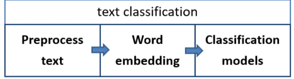
The process of text classification can be summarized as below

(10)

CHAPTER 2. TEXT CLASSIFICATION 10

Figure 2.1: Process of text classification

2.1 Dataset description

The dataset is provided by Sougo Lab which offers open source dataset for AI research. Sougo is subsidiary of Sohu company and it focuses on search engine, input method and high speed browser. The dataset includes news from different channels of Sohu news, the size is around 50MB, the text sample is as below.

(11)

2.2 Preprocess text

2.2.1 Extract content and label from raw news text

The first step of preprpcessing the raw text is extracting the prefix from URL as the label. From figure 2.1 we can tell, the URL of this news is

http://sports.sohu.com/20080607/n257351699.shtml

the first part of this URL ’sports’ means the news is from Sohu ’sports’ channel, thus extract ’sports’ as the label and all the text from ’content’ part.

2.2.2 Remove punctuation and stop words

There are punctuation, numbers, English letters in the text, and they con-tribute little to the text classification. Hence the regular regression is used to remove them. At the same time, stop words will also be removed, there are over 1000 stop words used in this thesis.

2.2.3 Segmentation

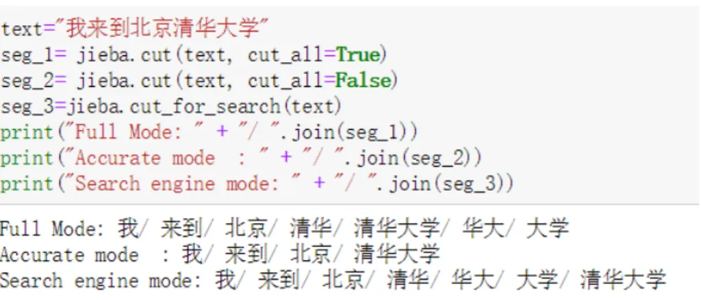
Word segmentation is the separation of the morphemes and also the same with tokenization for languages without ’space’ character. Chinese is very different from English and other alphabet languages. In English, words are separated by space, but there is no space between words in Chinese. In Chinese, one character can be a word, two or three characters can also make up a word, even 4 characters is also a word. Thus there are several ways to split a sentence,and it’s a big challenge to split the Chinese sentence. Jieba is an open source Python Chinese word segmentation library. It offers are 3 modes to do word segmentation.1

• Accurate mode

Trying to cut sentences most accurately which is suitable for text anal-ysis.

• Full mode

Scanning all the words that can be used as words in a sentence, is very fast, but it can not solve ambiguity.

(12)

• Search engine mode

On the basis of precise mode, user can segment long words again to improve recall rate, which is suitable for search engine word segmenta-tion.

For example, the sentence below means ”I came to Beijing Tsinghua univer-sity”, figure 2.3 shows the results of these 3 segmentation modes.

Figure 2.3: 3 modes of word segmentation

we can see from figure 2.3 that, if combine all the words in ’full mode’ and ’search engine mode’, the number of characters are more than the original sentence. The reason is, in these 2 modes, Jieba algorithm will extract every possible words from the sentence. However, the words in accurate mode merge together is the original sentence, thus in this thesis, accurate mode is taken to do word segmentation.

2.3 Word embedding

Words are map into vectors using word embedding models, Word embedding is a collection of statistical language modelling and techniques in NLP area[4]. It maps words and phrase to vectors of real numbers, they capture both semantic and syntactic information of words. Word embedding can be used to calculate word similarity which can be used in many tasks such as information retrieval. In the thesis, 4 ways are used for word embedding:

• Word2vec • Doc2vec

(13)

• Tfidf

• Deep learning embedding method

word2vec

Word2vec is a NLP technology which takes a text corpus as input and words are represented as vectors. The proximity in vector space indicates semantic or functional similarity [5]. The resulting word vector file can be used as features in many natural language processing and machine learning appli-cations. CBOW and Skip-gram are core algorithms of word2vec and they are very similar to some extent.The chart is the structure of CBOW and Skip-gram

Figure 2.4: Structure of CBOW and Skip-gram [5]

From figure 2.4 we can see, CBOW is used for predicting the current word while skip-gram predicts the words around the current word given the current word. In this thesis, I use skip-gram and the window size is set to be 5, the dimension of each word is set to be 100.

(14)

Doc2vec

Doc2vec model changes text document to numeric representations. Each sample is one vector, the dimension of the vector can be determined by user. Both word2vec and Doc2vec are unsupervised learning methods and Doc2vec was developed on the base of Word2vec. Doc2vec inherits the advantages of word2vec such as take semantic and word order into consideration. There are also 2 algorithms in Doc2vec which are Distributed Memory Model of Paragraph Vectors (PV-DM) and distributed bag of words (PV-DBOW)[6]. In this thesis, I use PV-DM, and the dimension of each text is set to be 300.

Tfidf

Tfidf(term frequency inverse document frequency) is a commonly used weighted technology for information retrieval and data mining. It is often used to mine keywords in articles, and the algorithm is simple.

Tf means term frequency, which is the the number of times that the word occurs in the document. Idf means inverse document frequency, which is a measure of how much information the word provides, and it is used to prevent some common words to have high term frequency but contribute little to the text such as ’a’ and ’the’. Tfidf can be calcuted as

tf idf =tf ×idf =tf ×log(N

df) (2.1)

here N means total number of documents in the text and df means the number of documents where the word appears[?].

Deep learning embedding layer

Every word in the corpus will be replaced by a number, the total number is the the number of words in the corpus, and it will be trained in the first layer in av deep learning model, which will introduce more in detail in deep learning model part.

(15)

2.4 Machine Learning and Deep Learning

Models

Machine learning models are the general inductive process automatically builds a classifier by learning from a set of preclassified documents.[7] The research of deep learning begins with artificial neural network, which aims to simulate the operation mechanism of human brain.[8]. The neural network opened up the research of deep learning theory in academic and industry. This series of developments have made breakthroughs in the fields of image speech recognition, automatic translation and NLP tasks[9].

In this thesis, machine learning methods such as Naive Bayes and SVM, deep learning methods such as CNN and RNN are used to classify the news. All the inputs have been mapped to word embeddings in the previous steps. And the output of these models is the news class which has the maximum probability. Loss function and optimizer are used to improve the model accuracy. The structure of all the models will be described in detail in chapter 3 and 4.

(16)

Chapter 3

Methods

Machine learning methods have been used in natural language processing area since last century. With the increasing popularity of deep learning, researchers turn their interest to high accuracy deep learning models.In this chapter, I will introduce the machine learning and deep learning models used in this thesis.

3.1 Naive Bayes

Beyes rule is used to calculate the posterior probability using prior probability which might be related. There are two events, event A and event B. The conditional probability (also known as a posterior probability) of event A under the condition that event B has occurred refers to the probability of event A occurring under the condition that event B occurs. The conditional probability can be expressed as P(A|B),P (B) is called a prior probability, P(A, B) is the joint probability of A and B.

p(A|B) = P(A, B) P(B) =

P(A)P(B)

P(B) (3.1)

if P(A|B) is equal to P(A),which meas the posterior probability of event A has nothing to do with event B, we can say event A and B are independent, otherwise, they are dependent [10].

In multiclass problem, the equation can be

(17)

CHAPTER 3. METHODS 17

P(Ci|X) =

P(X|Ci)p(Ci)

p(X) (3.2)

here C is the set of classes, and Ci refers to the ith class. and X is the input

text. For the given text, all the P(X) is equal because the the text is certain input. Thus the fraction above is proportional with the joint probability,the denominatorP(X|Ci)p(Ci) which according the chain rule can also be written

as

P(x1, x2...xm, Ci) =P(x1|x2, ....xn, Ci)P(x2|x3, ...xn, ci)...P(xn|Ci)P(Ci)

(3.3) Now the naive bayes algorithm assumes that all features in X x1, x2....xm

are mutually independent, which means P(x1|x2, ....xn, Ci) = P(x1|Ci), the

equation above can be written as

Qn

j=1P(xj|Ci)P(Ci). In naives bayes classifier, we try to find the class label

y=Ci which can get max posterior probability

ˆ y= arg max i∈C n Y j=1 P(xj|Ci)P(Ci) (3.5)

Naive Bayes classification algorithm was first proposed by Kuhns and Maron in 1960s and put into use in text classification and information retrieval. It is a supervised learning method. Naive Bayesian refers to two premises based on position independence and conditional independence. Obviously, the above two premises are not valid in the actual text, because the entries in the text are not independent of each other, they are interrelated, and the position of entries in the text is also related to the contribution to the text. However, these two premises will affect the results of Naive Bayesian classi-fication, Naive Bayes has shown good classification performance in practical applications, that is why Naive Bayes is widely used in machine learning area [11].

(18)

3.2 Support Vector Machine

Supportive vector machines(SVM) is a classifier defined by a separating hy-perplane. It is a supervised learning model, given labeled training data, the algorithm outputs an optimal hyperplane which can maximize the margin between 2 classes. SVM has its unique advantages in solving the problem of high-dimensional space vector and it is also memory efficient [12]. The system uses a hyperplane that has been found through training and learning to classify the sample space into two categories. When the problem to be solved is linearly separable, the optimal hyperplane requires the maximum of the optimal hyperplane based on the correct classification.

Multiclass SVM aims to assign labels to instances by using support vector machines, where the labels are drawn from a finite set of elements. In this thesis, Multisvm was trained with one-against-all approach. One-against-all approach builds as many binary classifiers as there are classes, each trained to separate one class from the rest. To predict a new instance, multisvm iterate each classifier until the first classifier which assigns the new instance as its class member is found [13].

3.3 Neural Network

Neural Network is a deep learning method which simulates human brain neu-ral network which can be used to do classification. Its structure is usually a three-layer network composed of input layer, hidden layer and output layer. The hidden layer can be multiple. Multilayer Perceptron(MLP) is a feedfor-ward neural network, the connection between layers are fully connected.

3.3.1 Activation Function

In a neural network, the output can be calculated as below

y=Xweight∗input+bias (3.6)

the value of y can be any value ranging from -inf to +inf. The neurons don’t know the bounds of the value. Thus activation function is used to decide whether the neuron should be fired or not. There are many choices of activation functions, 4 popular function are used in this thesis

(19)

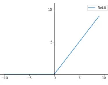
Relu

The ReLu function is as shown below, it gives an output x if x is positive and 0 otherwise.

f(x) =max(0, x) (3.7) the relu function can be drawn as figure 3.1

Figure 3.1: Function image of relu

For a network with random initialized weights and almost 50% of the network yields 0 activation because of the characteristic of reLu,the network then becomes lighter.

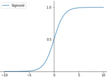
Sigmoid

The sigmoid function is

f(x) = 1

1 +e−x (3.8)

It will rescale the inputs to (0,1), it is a non-linear function,compared to infinity boudary of linear function, sigmoid can bound the output in a certain range. Sigmoid function is one of the most widely used activation functions nowadays.

(20)

Figure 3.2: Function image of sigmoid

Tanh

The equation of Tanh function is f(x) = e

x₋_e−x

ex₊_e−x (3.9)

It will rescale the inputs to (-1,1)

(21)

Tanh is also a non-linear function and the relationship between tanh and sigmoid is

tanh(x) = 2sigmoid(2x)−1 (3.10)

Softmax

The softmax function can convert a K dimension vector to another k dimen-sion vector,after applying softmax, each component will be in the interval (0,1), and the sum of components will be 1, the equation is

σ(z)i =

ezi

Pk

j=1ezj

(3.11)

In the equation above, i=1,2...K. In text classification, a deep learning model use softmax in a fully connection layer because it will get the probability of each class.

3.3.2 Loss Function

For a classification problem, cross entropy will compare the distribution of the predictions, which are the activations in the output layer, one for each class, with the true distribution. Usually, an activation function (such as Softmax) is applied to the scores before the cross entropy loss computation.

L(y,yˆ) = −

N

X

i=0

(yi∗log(ˆyi)) (3.12)

y is the true label and ˆy is the predicted label. Categorical cross entropy loss which is also called softmax Loss,it is a softmax activation plus a cross entropy loss. It will train a deep learning model to output a probability over the N classes for each input. It is often used for multi-class classification.

3.3.3 Optimizer

In a neural network, a optimizer is used to minimize the loss function. Adap-tive Moment Estimation(Adam) can be treated as a combination of RMSprop and Stochastic Gradient Descent(SGD) with momentum and take advantage of both methods. Adam is an adaptive learning rate method fist published

(22)

in 2014 [14], which means, it computes individual learning rates for differ-ent parameters. In Adam, there are several parameters should be initialized which areα, β1, β2.θ0 is the initial parameter vector,m0,v0and will initialized

as 0.The steps is as below. First, calculate the gradient at time t

gt=θ J(θt−1) (3.13)

update m and v by

mt=βtmt−1+ (1−β)gt (3.14)

vt =βtvt−1 + (1−β)gt2 (3.15)

the next step is to remove bias correction because m and v are initialized to 0 and the first few steps will make m and v close to 0.

ˆ m= m t 1−βt 1 (3.16) ˆ v = v t 1−βt 2 (3.17) and use ˆm and ˆv to update parameter θ

θt =θt−1−α ˆ mt ˆ vt+ε (3.18)

3.4 Convolutional Neural Network

Convolutional Neural Network(CNN) is a feedforward multi-layer network model, it is also a kind of artificial neural network. CNN has made great breakthroughs in the field of image recognition, Figure 3.4 shows the struc-ture of a classical CNN called LeNet5, it is used in [15] to classify digits. In a CNN model, a convolution layer has at least one convolution kernel(or filter) to do convolution operation. The destination element is the result of element-wise product and sum of the filter matrix and the original image. After the convolution layer, a pool layer is applied, a pool layer is used to do subsampling. The reason is that even after convolution, the image is still very

(23)

Figure 3.4: Architecture of LeNet, a convolutional neural network for digits recognition[15]

large because the convolution kernel is relatively small. In order to reduce the data dimension, subsampling is carried out. Even reducing much data, the statistical attributes of features can still describe the image. However, the reduction of data dimension can effectively avoid overfitting.In practical applications, pooling methods include max-pooling and mean-pooling. Adding a Fully-Connected(FC) layer is a cheap way of learning non-linear combinations of the high-level features as represented by the output of the convolution layer. The Fully-Connected layer is learning a non-linear func-tion in that space. The flattened output is fed to a feed-forward neural network and back-propagation(BP) applied to every iteration of training. Over a series of epochs, the model is able to classify them using the softmax classification technique.

The weight sharing mechanism reduces the complexity of the model while effectively controlling the number of weights, and also constrain the number of parameters, which is used to improve the performance of BP algorithm in training. Compared with MLP, the parameter will decrease a lot.

In the era of artificial intelligence(AI), the research of natural language pro-cessing (NLP) has successfully attracted the attention of people, and has become one of the important research directions at present. Neural network structures such as CNN have gradually been studied to solve the difficult problems in the application of NLP, and made relevant progress. In addi-tion, CNN was used by Shen et al. to deal with semantic emotional tasks in information retrieval[2], while Kalchbrenner et al. introduced CNN to study a different pooling method in sentence modeling [?]. The above research fully shows that CNN model has a strong development potential in NLP area.

(24)

3.5 Recurrent Neural Network

It is widely acknowledged that CNN performs well in image recognition. In an image, the neighboring pixels are irrelevant. Nevertheless, for a sentence, the context have connections. For example, a verb comes after a subject. The previous input will have affect on the next input. However, CNN can’t get deal with this kind of problem very well.

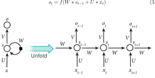
Recurrent Neural Network(RNN) is a type of artificial neural network de-signed to recognize patterns in sequences of data, such as text, genomes, the spoken word, or numerical times series data emanating from news, stock markets and government agencies [16]. In a RNN model, the hidden layer node is not just received from the input but also connect with the previous layer. Figure 3.5 shows how RNN work,the hidden layer value of s at time t can be calculated as

st=f(W ∗st−1+U ∗xt) (3.19)

Figure 3.5: RNN structure1

3.5.1 Long Short Term Memory

Long Short Term Memory(LSTM) is a variant of RNN, it was first intro-duced by Hochreiter and Juergen Schmidhuber [17]. LSTM is developed to solve the problem of gradient vanishing or explosion problem. Compare with

1 http://www.wildml.com/2015/09/recurrent-neural-networks-tutorial-part-1-introduction-to-rnns

(25)

RNN, LSTM has better performance in long sequence data. The structure of LSTM is shown in figure 3.6. there are 3 ’gates’ to control the output,

Figure 3.6: LSTM structure2

input gate(i), forget gate(f) and output gate(o). Wi_{, W}f_{, W}o _are

connec-tion weights between the previous hidden layer and current hidden layer, respectively, Ui_{, U}f_{, U}o _{are the weights for the input x at time t.}

it =σ(Uixt+Wiht−1) (3.20)

ft=σ(Ufxt+Wfht−1) (3.21)

ot=σ(Uoxt+Woht−1) (3.22)

These 3 gates have the same dimension. The output of the hidden layer ht

is a combination of these 3 gates. ˆ

C =tanh(Ugxt+Wght−1) (3.23)

Ct=σ(Ct−1ft+ ˆCit) (3.24)

ht=tanh(Ct)ot (3.25)

In a LSTM model, we can control the percentage of how much the input or the previous memory to impact the result. For an extremely example, we can set the forget gate as all 0 to ignore the old memory completely.

(26)

3.5.2 Gated Recurrent Network

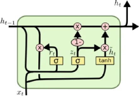
Gated Recurrent Network(GRU) is also a variant of RNN and but simpler than LSTM, it also performs good in NLP area [16]. GRU has 2 gates which are an reset gate and update gate compared with 3 of LSTM. The structure of GRU is as below

Figure 3.7: GRU structure3

the output of hidden layer at time t can be calculated as below

zt =σ(Uzxt+Wzht−1) (3.26) rt=σ(Urxt+Wrht−1) (3.27) ˆ h=tanh(Uhxt+Wh(rtht−1)) (3.28) ht = (1−zt)ht−1+ztht (3.29) 3_{https://isaacchanghau.github.io/post/lstm-gru-formula/}

(27)

Chapter 4

Experiment

In this chapter, the process of text classification experiment will be shown in detail. The goal of the experiment is to compare different models and find the model with the highest accuracy. I will describe the steps of preprocessing data, compare different word embedding models, introduce the structure of all the classification models and discuss the final results.

4.1 Experiment environment

The experiment is divided into 2 parts, the word embedding part and ma-chine learning models run in the author’s laptop. The deep learning models training is executed using Google Colaboratory which is an online coding platform offering free 1G GPU1_{, the coding language is Python, Scikit-learn}

is a library providing state-of-the-art implementations of many well known machine learning algorithms[18]

Tensorflow and Keras

Tensorflow is an open sourced software library for high performance numer-ical computation. It is widely used in deep learning and machine learning tasks, it offers APIs for developing, so the neural network code can be writ-ten in a few lines. Keras is a high-level neural networks API, writwrit-ten in Python and capable of running on top of TensorFlow, CNTK, or Theano. It

1_{https://colab.research.google.com}

(28)

CHAPTER 4. EXPERIMENT 28

was developed with a focus on enabling fast experimentation. The code was written in python using keras and tensorflow as backend.

4.2 Preprocess data

The dataset is a collection Chinese news, the first step is removing the punc-tuation, English letter, numbers and stop words which contribute little to the final classification. Chinese has no space between words, the second step is using Jieba library to do segmentation to split the text without any space to a list of words. Jieba is an open source Python Chinese word segmenta-tion library. The comparison of the raw text and after preprocessing data is shown in Figure 4.1

Figure 4.1: Comparison of raw text and after preprocessing

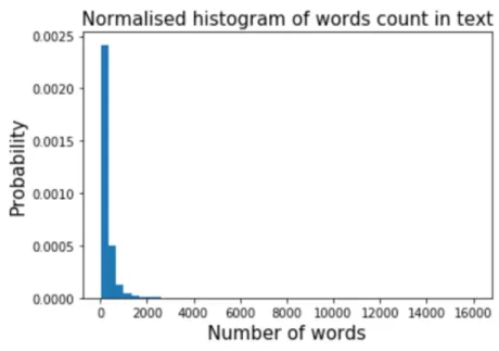
After preprocessing the dataset, each original news is transferred to a bag of words. I use number of words instead of length of the text because the characters in a word vary. In this thesis, I dismiss the news which are too short which has the number of words less than 50. Thus the shortest text has 50 words while the longest news has 15651 words, and the mean is 288. In total, there are 18464 samples in the whole dataset.I use 80% dataset as training set and 20% as test set, which are chosen randomly. The distribution of the number of words of the whole dataset is shown in Figure 4.2

we can see from Figure 4.2 that most of the text has the number of words less than 1000. To make it more clearly, Figure 4.3 shows the normalized

(29)

Figure 4.2: Normalised histogram of words count

histogram of words count under 1000. From figure 4.3 we can see most of the news have less than 400 words.

Figure 4.3: Normalised histogram of words count under 1000

After preprocessing these news, there are 14 different categories in total, which are

(30)

• 2008 (news related to Olympic held in Beijing, 2008) • auto(news related to cars)

• business

• cul(news related to culture) • health

• house • IT • learning

• mil.news(news related to military)

• news(realtime domestic and international news) • sports

• travel • women

• yule(news related to entertainment)

the quantity of news from different channels are showed in Figure 4.4:

(31)

We can see from the Figure 4.4 that the news from channels of sports,news, house and business are higher than the other channels. Military and cul-ture channel have the least news among all the channels. The imbalance of quantity of news will make the the classifier more difficult.

4.3 Word embedding

Word embedding methods are used to map words to numeric vectors which can be used for computation.There are 4 ways in this thesis to do word embedding, which is doc2vec, word2vec, tfidf and embedding layer trained in deep learning models.

The corpus is the collection of all the samples. Doc2vec method uses the corpus to train the doc2vec model, and use this model to map every sample to a fixed dimension vector. The dimension can be set manually. I set the dimension of text to be 300, then no matter how long the text is, the output is a 300 dimension numeric vector. The same corpus is used for word2vec method, after generating the word2vec model, every word will be mapped to a 100 dimension vector.

In keras, the first layer of a text classification task is embedding layer, there are 2 ways in this thesis to do word embedding. The first one is using word2vec to map words to vectors, each word is 100 dimension long. The second method is using function ’Tokenizer’ offered by keras, This function allows to vectorize a text corpus, by turning each text into a sequence of integers, each integer is the index of a token in a dictionary. Hence each sample text will be transferred to a bag of numbers. In the embedding layer of a deep learning model, the words will be trained and transferred to the next layer, the dimension of each word is set to be 100 here, the same as the word2vec method.

The deep learning models require the samples of input have same dimension, thus the text length is fixed to be 300 in this experiment. If the text is less than 300, zeros will be padded to the tail of the text, otherwise it will be cut, and the first 300 words will be reserved.

In scikit learn library, TfidfVectorizer is offered to map text to a numeric matrix. Each element is the tfidf value of the word. The rows represent the samples, and the columns represent the words. If the word appears in a sentence, the element will be a number, if not, it will be 0, which is similar to one-hot representation. Thus each row will have the length of the whole

(32)

corpus. The tfidf matrix has the dimension of (18464, 200400), 18464 is the number of samples, and 200400 is the number of words in the corpus, since the corpus is quite large, the tfidf matrix is very sparse. [19]

The dimension of each sample after these 4 methods is very different as table 4.1 shows

Table 4.1: Dimension of different word embedding model method dimension

Doc2vec 300

Word2vec 300*100 Tfidf corpus length Embedding layer 300*100

4.4 Feature selection

In text classification, large amount of text data is needed to train the classi-fier. There will be many feature items in a text, the dimension of the vector will be very high, which will increase the complexity of the classification Actually, in a high dimensional feature space, not every feature contributes to classification, many ambiguous features not only contribute little to the classification, but also increase the learning burden of classifiers and reduce classification accuracy. This noise will bring huge computation elimination in time and space for a classifier and also affects the accuracy of the classifier. In order to reduce the computational complexity of classification models, it is necessary to reduce the dimension of feature space. At present, the most commonly used dimension reduction technology of feature space is feature selection technology.

There are many ways to do feature selection, in this thesis, I pick up the top 50 words with highest tfidf value to represent the text and compare with the original text. The reason of feature selection is trying to find if feature selection influence the classifier and how it affects the classifier.

(33)

4.5 Accuracy

To compare different models, accuracy is used to recognize whether the model performs well. Accuracy is the rate that the number of test samples that have the predicted class labels equals to the original labels.

4.6 Results of experiment

There are 4 ways to do word embedding, and there are 10 machine learning and deep learning models to do classification, thus there will be many com-bination of these methods in these two parts. In this section,I will introduce the model structure and the result of each model and then compare them together.

4.6.1 Machine learning models

Tfidf+NB

This model takes tfidf as the word embedding method and naive bayes(NB) as its classification model

Tfidf+feature selection+NB

This model takes Tfidf as word embedding method, and use top 50 words with high tfidf value to do feature selection and Naive bayes as its classification method.

Tfidf+SVM

This model takes tfidf as the word embedding method and SVM as its clas-sification model

(34)

Tfidf+feature selection+NB

This model takes Tfidf as word embedding method, and use top 50 words with high tfidf value to do feature selection and SVM as its classification method.

Doc2vec+NB

This model takes doc2vec as the word embedding method and naive bayes as its classification model

Doc2vec+feature selection+NB

This model takes doc2vec as word embedding method, and use top 50 words with high tfidf value to do feature selection and Naive bayes as its classifica-tion method.

Doc2vec+SVM

This model takes tfidf as the word embedding and SVM as its classification model

Doc2vec+feature selection+SVM

This model takes doc2vec as word embedding method, and use top 50 words with high tfidf value to do feature selection and SVM as its classification method.

the accuracy of the above models is shown in table 4.2

We can see from the table 4.2 that, when using doc2vec as word embeddings, the text classification get very low accuracy. On the contrary, tfidf performs better, but tfidf matrix can get very sparse due to its mechanism. SVM has better result than naive bayes, but it is a very time consuming way to do classification compared to naive bayes. For feature selection, we can see the accuracy between models with feature selection and without feature selection is close, which means under feature selection, the complexity and time consuming is much lower, but the accuracy doesn’t decrease much.

(35)

Table 4.2: Accuracy of machine learning models

Model Accuracy(%) Tfidf+NB 70.84 Tfidf+feature selection+NB 73.59 Tfidf+SVM 84.29 Tfidf+feature selection+SVM 84.55 Doc2vec+NB 21.6 Doc2vec+feature selection+NB 20.82 Doc2vec+SVM 21.58 Doc2vec+feature selection+SVM 21.58

4.6.2 Deep learning models

All the deep learning models take categorical cross entropy as loss function, adam as optimizer,batch size is 1000 and each model will run 20 epochs. For each algorithm, the pretrained word2vec embeddings and without pretrained embeddings are the input layer of these models separately. Embeddings without pretrained will be trained at the first layer, on the contrary, word2vec embeddings will be transferred to the next layer directly.

Multilayer Perceptron(MLP)

There are 3 layer in this MLP model as Figure 4.5 shows, the input layer is the word vectors, the hidden layer includes 1000 nodes and uses relu as activation function and has 50% dropout, the output layer is a fully connected and uses softmax as the activation function.

Convolutional Neural Network(CNN)

The structure of this CNN model is shown in figure 4.6, the first layer is a convolutional layer, there are 256 filters and each filter size is 5*5 and then followed by a max pool layer with size 3*3. The third layer is another con-volutional layer with 128 filters with 3*3 size, and followed by a max pool layer with size 3*3. The fifth layer is also a convolutional layer, there are 64 filters in this layer and each kernel is 3*3 size, then after these convolutional and pooling layers, there is a flatten layer to flatten these multi dimensional vectors, after that, there is a hidden layer with 256 units, and its fully

(36)

con-CHAPTER 4. EXPERIMENT 36

Figure 4.5: MLP structure

nected and the activation is relu, and the output layer is the number of labels with softmax activation.

(37)

Long Short-Term Memory(LSTM)

The structure of LSTM has been explained in chapter3,in this LSTM model, the hidden layer units are 300, activation is tahn, and recurrent activation is sigmoid, dropout is 20% and the units to drop for the linear transformation of the recurrent state is 10%.

Gated recurrent units (GRU)

In this GRU model,the hidden layer units are 256, activation is tahn, and recurrent activation is sigmoid, dropout is 20% and the units to drop for the linear transformation of the recurrent state is 10%.

2 layer GRU

In this GRU model,there are 2 hidden layer with the previous GRU model structure, the output of the first layer is the input of second hidden layer.

TextCNN

This model is first introduced by Yoo Kim in 2014 [20], he introduced a way to combine 3 filters with different size, which is 3*3,4*4 and 5*5, so they can handle different length short text. And then concatenate the results after these 3 filters. The next layer is a fully connected layer and the output layer, the structure is shown in figure 4.7.

CNNGRU

This model makes a combination of CNN and GRU, the output of CNN is the input of GRU, the structure is shown in figure 4.8

CNNGRU Merge

This model also makes a combination of CNN and GRU like the previous model, the difference is the combination method. The previous model is

(38)

Figure 4.7: TextCNN model structure[20]

Figure 4.8: CNNGRU model structure

a sequential model, but CNNGRU Merge model is the concatenate of the result of CNN and GRU, the structure is shown in figure 4.9.

The accuracy of the models above is in table 4.3, accuracy with pretrained embedding means the embedding layer take word embeddings using word2vec method.

From table 4.3 we can see, compared with traditional machine learning method, all of deep learning methods performs better. In the above deep learning method, 2 layer GRU with pretrained word embeddings gets the highest accuracy which is 93%. The ’CNNGRU with pretrained word em-beddings’ and ’CNNGRU Merge’ model also have very high accuracy which are 92.7% and 92.6% separately. The accuracy of ’CNN’ and ’CNNGRU’ are lowest compared to other models, which is only 86%.

(39)

Figure 4.9: CNNGRU Merge model structure Table 4.3: Accuracy of deep learning models

Model Accuracy(%) Accuracy(%) with pretrained embedding

MLP 88.4 87.7 CNN 86.0 88.2 LSTM 86.7 87.2 GRU 89.0 91.8 2 layer GRU 86.1 93.0 TextCNN 91.2 87.4 CNNGRU 86.0 92.7 CNNGRU Merge 92.6 90.6

Visualize the training history

TO visualize the training history, the loss and accuracy matrix are used to show the change in each epoch. Figure 4.10 is the training loss and training accuracy of model MLP.

(40)

Figure 4.10: Training loss and training accuracy of model MLP that’s why the result become stable after the 3rd epoch.

Confusion Matrix

In the field of machine learning, a confusion matrix is a table that is often used to describe the performance of a classification model, Each row of the matrix represents the instances in a predicted class while each column represents the instances in an actual class. In a confusion matrix,it is easy to see which class was wrongly classified, and the correlationship between different classes. The confusion matrix in Figure 4.11 is the visualization of the text classification of model MLP.

From Figure 4.11 we can see, most of the wrongly classified labels came into class ’news’, because the news channel is the collection of different kinds of real time news, it relates to the news from all channels such as sports and business, so it is reasonable if a sports news came to the ’news’ channel. If the dataset can be more clearly classified, the accuracy will get higher. There is also a intersection between’2008’ and ’sports’ because the news from channel 2008 is about the Olympic Games, which is also can be related to ’sports’, they share some key words.

4.6.3 Half sized and double sized dataset

To verify the idea that whether the dataset size will affect the accuracy of models, I choose 2 dataset which is half size and double size of the original dataset. Half sized dataset is choosing half of the original files, and double

(41)

Figure 4.11: Confusion matrix of MLP

sized is using the files from the same source which can be downloaded from Sougo Lab. After doing experiments using deep learning models, table 4.4 and 4.5 show the results separately.

Compared with normal sized dataset, half sized dataset get lower accuracy. After checking the accuracy and loss history charts, it is easier to get over-fitting using half sized datset. By contrast, most of the accuracy of double sized dataset is over 90%, there is a big improvement if compared with half size dataset. When comparing with normal sized dataset, most of the models get higher accuracy. It is clear to see the model with the highest accuracy is

(42)

Table 4.4: Accuracy of deep learning models using half sized dataset Model Accuracy(%) Accuracy(%) with pretrained embedding

Table 4.5: Accuracy of deep learning models using double sized dataset Model Accuracy(%) Accuracy(%) with pretrained embedding

2 layer GRU with pretrained word2vec embeddings for both half sized and double sized dataset, which is the same with normal sized dataset.

4.7 Analysis and discussion

The experiment has 3 steps, except the first step ’preprocess text’, there are several choices of the second step ’word embedding’ and the third step ’classi-fication models, in the whole experiment, there are 24 different combinations in total.

For the word embedding part, Doc2vec word embedding has the lowest accu-racy which is only around 20%, it is too low to be accepted. Thus for short text, Doc2vec is not a good choice for word embedding. Tfidf method will a produce very sparse matrix which takes much disk space. Furthermore, if the vocabulary has a new word, it have to be trained again, and the dimen-sion will also change. Word2vec has the same drawback, a new word will

(43)

cause the retraining of the whole vocabulary. However, it can be avoided by assigning initial values to a new word, for example, all zeros. However, this method will impact the correlation of the new word with its context.

Compared with machine learning models such as Naive Bayes and SVM, all the deep learning models have higher accuracy. However, naive bayes is much less time consuming compared to SVM and other deep learning models, but it still has the accuracy around 70%.

For deep learning models, there are 2 input ways, which are pretrained word2vec embeddings, and the embedding layer needs to be trained. From the result we can see, It’s hard to conclude which is better, every method has its advantages.

MLP model has the simplest structure, but from the results we can see, the simplest model is not the worst. The structure of a model determines the model complexity, which means, the running time and space will also be affected.

2 layer GRU with pretrained word2vec embedding has the highest accuracy within all the models using the normal sized dataset. It is the same for half sized dataset and double sized dataset. It performs very well for the Sohu news dataset.

The limitation of the experiment is, it is hard to execute the experiment in all the Chinese news dataset, thus it is a hint for Chinese news classification, but strictly speaking, it is not the best for all the Chinese news. The dataset size, the length of news, the complexity of models will also have an impact on the result.

(44)

Chapter 5

Conclusions

With the development of machine learning and deep learning, text classifica-tion comes into a new generaclassifica-tion, the accuracy is higher and the time con-suming is lower. In this thesis, the process of text classification is introduced, which includes 3 parts, preprocess text, word embeddings and classification models. Chinese news is chosen to be the dataset, which is a collection of news from different channels from Sohu company .The preprocess part in-cludes removing punctuation, English letters, numbers and stopwords. After that, the news will be segmented to a list of words. There are 4 ways to do word embedding which are doc2vec, word2vec, tfidf and embedding layer. In the classification models, 2 machine learning models and 8 deep learning models are taken to do classification. At the same time, There is a com-parison between whether adding feature selection, whether using pretrained word embeddings, which also produce more combinations of the models. The ’2 layer GRU model with pretrained word2vec embeddings’ model gets the highest accuracy.

In this thesis, the hypothesis of whether the volume of the dataset will impact the accuracy is also discussed. The same models are used for half sized and double sized dataset from the same source. The results show the accuracy of half sized dataset is lower compared to normal sized dataset. On the contrary, double sized dataset gets higher accuracy in most of the models˜a The dataset is relatively small compared to the data size in a real company. From the time consuming, the accuracy, the space the matrix takes, the dataset, all the aspects will affect the final choices in the real industry. Text classification not only can be used in news classification as described in this thesis, but also in other areas such as spam detection and sentiment

(45)

CHAPTER 5. CONCLUSIONS 45

analysis. It will surely help people save time and easy to find what they need. The development of natural language processing and big data also have a good impact on text classification, which will make the classification faster and more accurate.

(46)

Bibliography

[1] H.P. Luhn. Key word–in–context index for technical literature (kwic index). American Documentation, pages 288–295, 1960.

[2] G. Salton, A. Wong, and C. S. Yang. A vector space model for automatic indexing. Commun. ACM, 18(11):613–620, November 1975.

[3] Eva Gibaja and Sebasti´an Ventura. A tutorial on multilabel learning.

ACM Comput. Surv., 47(3):52:1–52:38, April 2015.

[4] Yoshua Bengio, Holger Schwenk, Jean-Sébastien Senécal, Fréderic Morin, and Jean-Luc Gauvain. Neural Probabilistic Language Models, pages 137–186. Springer Berlin Heidelberg, Berlin, Heidelberg, 2006. [5] Tomas Mikolov, Kai Chen, Greg Corrado, and Jeffrey Dean. Efficient

estimation of word representations in vector space. ICLR(International Conference on Learning Representations), 2013.

[6] Quoc Le and Tomas Mikolov. Distributed representations of sentences and documents. In Proceedings of the 31st International Conference on International Conference on Machine Learning - Volume 32, ICML’14, pages II–1188–II–1196. JMLR.org, 2014.

[7] Fabrizio Sebastiani. Machine learning in automated text categorization.

ACM Comput. Surv., 34(1):1–47, March 2002.

[8] Wissal Farsal, Samir Anter, and Mohammed Ramdani. Deep learning: An overview. In Proceedings of the 12th International Conference on Intelligent Systems: Theories and Applications, SITA’18, pages 38:1– 38:6, New York, NY, USA, 2018. ACM.

[9] T. Young, D. Hazarika, S. Poria, and E. Cambria. Recent trends in deep learning based natural language processing [review article]. IEEE Computational Intelligence Magazine, 13(3):55–75, Aug 2018.

(47)

BIBLIOGRAPHY 47

[10] Andrew Gelman, John B. Carlin, Hal S. Stern, David B. Dunson, Aki Vehtari, and Donald B. Rubin. Bayesian Data Analysis 3rd Edition. Chapman and Hall/CRC, 2013.

[11] Eibe Frank and Remco R. Bouckaert. Naive bayes for text classification with unbalanced classes. In Johannes F¨urnkranz, Tobias Scheffer, and Myra Spiliopoulou, editors, Knowledge Discovery in Databases: PKDD 2006, pages 503–510, Berlin, Heidelberg, 2006. Springer Berlin Heidel-berg.

[12] Fabrice Colas and Pavel Brazdil. Comparison of svm and some older classification algorithms in text classification tasks. In Max Bramer, editor, Artificial Intelligence in Theory and Practice, pages 169–178, Boston, MA, 2006. Springer US.

[13] Chih-Wei Hsu and Chih-Jen Lin. A comparison of methods for multi-class support vector machines. IEEE Transactions on Neural Networks, 13(2):415–425, March 2002.

[14] Diederik Kingma and Jimmy Ba. Adam: A method for stochastic op-timization. International Conference on Learning Representations, 12 2014.

[15] Yann Lecun, Leon Bottou, Y Bengio, and Patrick Haffner. Gradient-based learning applied to document recognition. Proceedings of the IEEE, 86:2278 – 2324, 12 1998.

[16] Kyunghyun Cho, Bart van Merri¨enboer, Caglar Gulcehre, Dzmitry Bah-danau, Fethi Bougares, Holger Schwenk, and Yoshua Bengio. Learning phrase representations using RNN encoder–decoder for statistical ma-chine translation. In Proceedings of the 2014 Conference on Empirical Methods in Natural Language Processing (EMNLP), pages 1724–1734, Doha, Qatar, October 2014. Association for Computational Linguistics. [17] Sepp Hochreiter and J¨urgen Schmidhuber. Long short-term memory.

Neural Comput., 9(8):1735–1780, November 1997.

[18] F. Pedregosa, G. Varoquaux, A. Gramfort, V. Michel, B. Thirion, O. Grisel, M. Blondel, P. Prettenhofer, R. Weiss, V. Dubourg, J. Vander-plas, A. Passos, D. Cournapeau, M. Brucher, M. Perrot, and E. Duch-esnay. Scikit-learn: Machine learning in Python. Journal of Machine Learning Research, 12:2825–2830, 2011.

(48)

BIBLIOGRAPHY 48

[19] Wen Zhang, Taketoshi Yoshida, and Xijin Tang. A comparative study of tf*idf, lsi and multi-words for text classification. Expert Systems with Applications, 38(3):2758 – 2765, 2011.

[20] Yoon Kim. Convolutional neural networks for sentence classification.

Text classification Based on Machine Learning Methods

Text classification Based on Machine

Learning Methods

Acknowledgements

Abbreviations and Acronyms

Contents

Chapter 1

Introduction

1.1

Overview

1.2

Research problem

1.3

Structure of the thesis

Chapter 2

Text classification

2.1

Dataset description

2.2

Preprocess text

2.2.1

Extract content and label from raw news text

2.2.2

Remove punctuation and stop words

2.2.3

Segmentation

2.3

Word embedding

word2vec

Doc2vec

Tfidf

Deep learning embedding layer

2.4

Machine Learning and Deep Learning

Models

Chapter 3

Methods

3.1

Naive Bayes

3.2

Support Vector Machine

3.3

Neural Network

3.3.1

Activation Function

Relu

Softmax

3.3.2

Loss Function

3.3.3

Optimizer

3.4

Convolutional Neural Network

3.5

Recurrent Neural Network

3.5.1

Long Short Term Memory

3.5.2

Gated Recurrent Network

Chapter 4

Experiment

4.1

Experiment environment

Tensorflow and Keras

4.2

Preprocess data

4.3

Word embedding

4.4

Feature selection

4.5

Accuracy

4.6

Results of experiment

4.6.1

Machine learning models

Tfidf+NB

Tfidf+feature selection+NB

Tfidf+SVM

Tfidf+feature selection+NB