Improving the A-Contrario computation of a fundamental matrix in computer vision

Title: Improving the

A Contrario

Computation of a

Fundamental Matrix in Computer Vision

Author: Ferran Espuny Pujol

Advisor: Lionel Moisan

Tutor: Pedro Francisco Delicado Useros

Department: EIO – Estadística i Investigació Operativa

Academic year: 2014

MSc in Statistics and

Operations Research

Universitat Polit `ecnica de Catalunya

Facultat de Matem `atiques i Estad´ıstica

MSc in Statistics and Operations Research

Master’s Degree Thesis

Improving the

A Contrario

Computation of

a Fundamental Matrix in Computer Vision

Ferran Espuny Pujol

Lionel Moisan (Advisor)

MAP5 – Math´ematiques Appliqu´ees `a Paris 5 Universit´e Paris Descartes (UMR 8145) Pedro Francisco Delicado Useros (Tutor) EIO – Estad´ıstica i Investigaci´o Operativa

Contents

2 General Framework.Computer Vision Geometry 7 2.1 Camera Model . . . 7

2.1.1 Projective Formulation . . . 9

2.2 Point Features: Detection and Matching . . . 9

2.3 Epipolar Geometry and Fundamental Matrix . . . 10

2.3.1 The (Normalised) Seven-Point Algorithm . . . 12

2.3.2 Matching Error Evaluation Using the Fundamental Matrix 13 2.3.3 A Numerical Example . . . 14

2.4 Applications of the Fundamental Matrix . . . 15

2.4.1 Evaluating the Error in a Set of Matches . . . 15

2.4.2 Robust Matching . . . 15

2.4.3 Object Recognition . . . 15

2.4.4 3D Reconstruction and/or Camera Motion Estimation . . . 16

2.4.5 Camera Self-calibration . . . 16

2.4.6 Dense Matching Via Image Rectification . . . 16

3 Data Computation.SIFT Detection and Matching 19 3.1 Harris Corner Detection and Sub-Pixel Refinement . . . 19

3.2 Scale-Space . . . 20

3.3 SIFT Features . . . 21

3.3.1 SIFT Keypoints: Localisation . . . 21

3.3.2 SIFT Keypoints: Orientation . . . 22

3.3.3 SIFT Descriptors . . . 23

3.4 SIFT Matching and Limitations . . . 23

3.4.1 Matching Algorithm . . . 23

3.4.2 Limitations . . . 24

vi Contents

3.5 A Case of Study (1/2) . . . 25

4 Fundamental Matrix Computation.A Myriad of Methods 27 4.1 Methods for Inlier Data . . . 28

4.1.1 Algebraic Error Minimisation . . . 28

4.1.2 Geometrically-Based Error Minimisation . . . 30

4.2 Robust methods: Overview . . . 30

4.2.1 Numerical Methods: M-estimators and Case-Deletion Dia-gnostics . . . 31

4.2.2 The Random Sampling Consensus (RANSAC) Method . . 31

4.3 Random Sampling Methods.The RANSAC Family. . . 32

4.3.1 Optimisation Criterion . . . 32

4.3.2 Noise Scale Estimator . . . 33

4.3.3 Sampling Strategy . . . 33

4.3.4 Hypothesis Verification (Pre-validation) . . . 34

5 ORSA: An Outstanding Random Sampling Method 37 5.1 A ContrarioGeometric Detection and the Helmholtz Principle . . 37

5.2 Fundamental Matrix Computation using ORSA . . . 38

5.3 ORSA Performance and Limitations . . . 40

6 A New AC Method for Robust Matching and Fundamental Matrix Es-timation 43 6.1 Method Overview . . . 44

6.2 Line Distribution Pre-Computation . . . 45

6.2.1 Kernel Density Estimation of the Image Distribution . . . 45

6.3 A ContrarioStep . . . 46

6.4 Error Measures . . . 48

6.4.1 Optimal Geometric Error . . . 48

6.4.2 Comparing a Fundamental Matrix with Ground Truth . . 48

6.4.3 Comparing a Relative Camera Motion with Ground Truth 49 6.5 Evaluation . . . 50

6.5.1 Simulation . . . 50

6.5.2 Real Image Experiments . . . 52

Conclusion 59 Appendix.Projective Geometry 61 General Projective Geometry . . . 61

Affine Geometry . . . 64

Euclidean Geometry . . . 65

Bibliography 67

Preface

There exist numerous methods available for the robust computation of the funda-mental matrix given a set of putative point matches between two images. Unfortu-nately, it is not obvious which of the existing methods performs better or is more suitable given a particular set of matches. The simulations and real-image com-parisons found in publications are usually limited and ”old” methods tend to be forgotten in favour of new ones.

I discovered the ORSA method when I attended a seminar in Grenoble, three years ago. I perfectly remember from that talk that I was instantly attracted by the non-parametrica contrarioprobabilistic framework, which is based on the Helm-holtz perception principle and Gestalt theory. When I then looked for the first time at Mosian and Stival’s paper [MS04], I was moreover impressed by the perform-ance analysis and its outcome. In particular, more than a 80% of outliers were allowed for datasets of size around 250, which was a more than good performance with respect to the available matching methods . . . and the paper was dating back to 2004!

Investigating the possibility of extending the ORSA to go further is the main motivation of this research, which was conducted under the supervision and with the collaboration of Lionel Moisan (MAP5) and Pascal Monasse (IMAGINE), dur-ing a post-doctoral contract with the Callisto project, funded by the Agence Na-tionale de la Recherche (ANR-09-CORD-003), on the application of perception principles and statistical methods (a contrario) to computer vision. The advice of Pedro Delicado (EIO) and the background provided some time ago by Jos´e Ignacio Burgos Gil (ICMAT) have also been very helpful.

This book is an extended and improved version of the conference paper [EMM13], and it contains original work that has not been published elsewhere. An effort has been made to provide a self-contained text to make accessible the strongly interdis-ciplinary subject of computing in an automatic and robust manner the fundamental matrix tensor from a given a set of SIFT matches between two images.

Chapter 1

Introduction

1.1

Overview

Matching features between two images is an important task in Computer Vision [HZ04, Low04]. Exactly matching points satisfy theepipolar constraint, that is characterised in projective coordinates by a3×3matrix, thefundamental matrix. Given a set of potential point matches, some being corrupted by noise and some being wrong (outliers), we address the problem of determining the subset of cor-rect matches (inliers1) and the robust computation of the associated fundamental matrix.

Geometrically, the fundamental matrix expresses the fact that for a point in one image, its matching point in the other image can only be on a line (and not anywhere on that image) which is the image of the back-projection ray of the initial point; see Figure 2.2 to visualise the re-projected (F x) back-projection (Cx) of a pixel (x). Moreover, the fundamental matrix encodes information both about the internal camera calibrationand the relative displacement between the image frames (camera motion).

Accordingly, the fundamental matrix can be used not only to check the consist-ency between a set of potential matches (robust matching) or to recognise a given pattern in an image database, as explained below. Given a set of matches, the fun-damental matrix is broadly used as well to recover both the associated 3D points and camera positions (3D reconstruction), or just the latter (motion estimation), or the latter and the camera internal calibration (camera self-calibration). Finally, it can be also used torectifya pair of images (stereo rectification) so that the search for new matches is reduced to horizontal 1D search operations (stereo matching).

We will use the Scale Invariant Feature Transform (SIFT), which was con-ceived by David G. Lowe [Low04] with the purpose of recognising the instances of a query object in an image database. In particular, this feature descriptor was

1_{According to [UNE00], an inlier is a data value that lies in the interior of a statistical distribution}

and is in error, and an outlier is a data value that lies in the tail of the statistical distribution of a set of data values. Nonetheless, we use these words as done commonly in Computer Vision, where inlier means correct or valid data and, in contrast, outlier means incorrect data [HZ04].

2 Introduction

designed to allow changes in scale, and changes up to a certain degree in the im-age geometry (affine motions) and illumination. A SIFT feature is composed of a keypoint localisation in the image (the point coordinates that we are interested in), a scale, an orientation, and an array descriptor with local gradient informa-tion around a square window centred at the keypoint and oriented with the feature orientation.

Lowe performed the recognition task as follows. In a first step, features in the query object where matched with features in the database of images (using the Euclidean distance between features); these matches were then refined with the help of a geometric test. images with at least three matching features were retained. We will use SIFT point matches (ignoring the rest of the descriptor, which is less precise) as input data for the robust estimation of the fundamental matrix.

Algebraically, the fundamental matrix is a bilinear tensor of rank two between two-dimensional projective spaces. In particular, a minimum of seven point matches (not being in a degenerate configuration) are needed to determine a fundamental matrix. The difficulties for its robust computation can be listed as follows:

• 7matches are needed to determine a fundamental matrix using the epipolar constraints and the rank two constraint;

• the (algebraic) epipolar constraint is quadratic in the coordinates of the image matches, giving heteroscedastic residuals, and linear in the coefficients of the fundamental matrix;

• the rank-two constraint has degree 3 on the coefficients of the fundamental matrix, being non-convex; if imposed parametrically, the complexity of the epipolar constraint increases;

• the linear formulation in the image projective frames becomes a rational for-mulation when the geometric fitting errors are computed for minimisation;

• inlier ratios (ratio of correct matches) can be typically much below 50%, and outliers (wrong matches) do not follow a predictable distribution.

Philip H.S. Torr and David W. Murray proposed and compared in [TM97] sev-eral robust estimation techniques for the fundamental matrix. These techniques included M-estimators, case-deletion diagnostics and random sampling methods like Least Median Squares (LMedS) [Rou84] and Random Sampling Consensus (RANSAC) [FB81]. RANSAC (explained below) was used if the noise scale could be estimated, and LMedS otherwise when the inlier ratio could be below a 50%. The two random sampling methods gave the best performance, and M-estimators were successful only when given good initial estimates. Consequently, Torr and Murray proposed to use first a random sampling algorithm and then use the solution to initialise M-estimators. Since then, many variants of the parametric RANSAC method have been developed but the method is still being used in modern and ef-fective 3D reconstruction software, e.g. Bundler [SSS07].

Organisation 3

The Random Sample Consensus (RANSAC) [FB81] performs random sampling of at mostN minimal subsets of data (7-uples of matches) to hypothesise models. Each hypothetical model is evaluated using the point matches whose residual is under a user-specified threshold τ (these matches are the estimated correct ones, i.e. inliers), and the model that leads to the maximum number of estimated inli-ers is chosen (the final model is then re-estimated using only these inliinli-ers). The cost function that RANSAC tries to optimise assigns 0 to those matches with error under the thresholdτ (inliers) and a constant penalty otherwise [TZ00]. An inlier ratioεis usually user-specified to decide the number of random trialsN, although this decision can also be taken adaptively using the best model found so far [HZ04]. The Optimised Random Sampling Algorithm (ORSA) was proposed by Lionel Moisan and B´erenger Stival in [MS04]. It assumes a uniform spatial distribution of the features over the image. Through random sampling, it looks for a set of matches that is the least expected in terms of the precision achieved for a given number of inliers (a contrariocriterion). It requires as parameter only the maximum number of random trials to perform (that is, the computational effort allowed by the user). The actual number of random trials can drop to as little as 10% of the specified one when a “sufficiently good” model is found early (acceleration strategy). It can be seen as a non-parametric version of RANSAC, where all possible inlier thresholds are implicitly used (and compared) thanks to thea contrariocriterion.

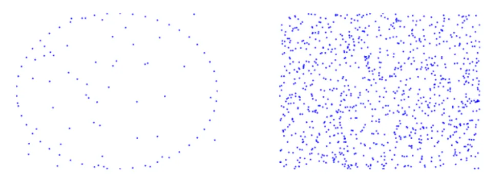
ORSA has been shown to outperform a fixed-threshold RANSAC approach and classical methods like M-estimators and LMedS, in particular by its ability to deal with very high outlier ratios [MS04,MMM12b]. However, performance lacks and even failure cases can be observed when the data points are far from being uniformly distributed, in particular when most of them lie in a small region of the image domain [MS04]. In the search for an adaptive improvement of ORSA, we will study the replacement of the uniform distribution of the ORSA method with an empirical distribution estimated non-parametrically using kernel methods with plug-in band-width estimation [SJ91].

We only carry out a preliminary comparison with the RANSAC and ORSA methods, the latter’s source code being available online2. Comparison with other modern methods was not possible due to the lack of available code. A major differ-ence between the proposed approach and almost all existing ones is that we build a model of the distribution of 2D image features to recover an optimal threshold, in-dependently of any matching, whereas other methods propose a model of (at best) the distribution of the 1D errors associated to the 2D matches.

1.2

Organisation

In Chapter2we present the general Computer Vision Geometry framework for 3D reconstruction. Namely, the pinhole camera model, the detection and matching of point features, and the two-view fundamental matrix tensor and its applications,

2

4 Introduction

among which the 3D reconstruction of an input set of matching points.

We devote Chapter3to explaining how the data is obtained and its character-istics. Mostly, the goal of the chapter is to present the SIFT feature detection and matching algorithms, and to analyse a bit the associated outcome.

Chapter4addresses the computation of a Fundamental Matrix given a set of point matches. It gives an overview on methods both for only inlying data and for robust methods able to handle outlying data, among which RANSAC merits a detailed explanation because of its good performance; then, it provides a taxonomy and brief survey on the many existing random sampling robust methods.

Thea contrarioapproach and the ORSA method will be presented in Chapter5, which finishes with a summary of performance highlights and a brief comment on its limitations. These contents merit a separate chapter since we build our method on top of them.

In Chapter 6 we present our modification of ORSA for, given a set of point matches, robustly compute the fundamental matrix and detect the subset of inlier matches; evaluation experiments are also summarised.

After Conclusion, the interested reader can consult an Appendix where the needed contents of Projective Geometry are formally summarised. In order to easy the comprehension of the text for readers not used to projective geometry concepts, we introduce next the minimum amount of notation and definitions required.

1.3

Notations

Any vector will be understood to be a column matrix by default:

u= (x1, x2, . . . , xn)T ⇔ u=    x1 .. . xn    . (1.1)

A vertical line will sometimes be used when combining matrices and vectors in blocks, in order to clearly separate the different blocks. For instance, a matrix composed by two “column” sub-blocksA1andA2can be denoted by(A1|A2).

We will use'to denote equality up to a scale factor. For any3-vectoru,[u]×

will be used to denote the antisymmetric matrix associated to thecross product(or vector product) ofuby any other 3-vectorv:

[u]×v=u×v . (1.2) concisely, ifu= (a, b, c)T_{, then} [u]×=   0 −c b c 0 −a −b a 0   . (1.3)

Notations 5

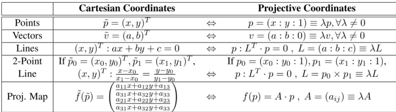
Cartesian Coordinates Projective Coordinates

Points p˜= (x, y)T _{⇔ p= (x:y: 1)≡λp,∀λ6= 0 (1.4)} Vectors ˜v= (a, b)T _{⇔ v= (a:b: 0)≡λv,∀λ6= 0 (1.5)} Lines (x, y)T _{:ax+by+c= 0 ⇔ p:L}T _{·p= 0, L= (a:b:c)≡λL (1.6)} 2-Point Ifp˜0 = (x0, y0)T,p˜1 = (x1, y1)T, Ifp0 = (x0 :y0 : 1), p1 = (x1:y1 : 1), Line (x, y)T _: x−x0 x1−x0 = y−y0 y1−y0 ⇔ p:L T _{·p= 0, L=p} 0×p1 ≡λL (1.7) Proj. Map f˜(˜p) = a11x+a12y+a13 a31x+a32y+a33 a21x+a22y+a23 a31x+a32y+a33 ! ⇔ f(p) =A·p , A= (aij)≡λA (1.8)

Table 1.1: Correspondence between Cartesian and projective notations on a plane for points, vectors, lines and projective maps.

1.3.1 Cartesian-Projective “Dictionary”

On a plane, many computations are eased by taking projective coordinates. With respect to Cartesian coordinates (in a possibly non-orthonormal affine coordinate frame), takingprojective coordinatescorresponds to adding a third coordinate to a point or a vector, its value being 1 or 0, respectively; see equations (1.4) and (1.5) in Table1.1. In fact, points and vectors are represented using 3 coordinates having a scale factor ambiguity, which in practice means that distance information is lost when using a projective framework. Line equations on a projective plane are also represented using 3 coordinates (1.6) and the line joining two points is given by the cross product of those points in projective coordinates (1.7). Note that all these projective elements are well defined independently of an arbitrarily selected scale factor.

A planar projective map is a transformation from a plane to a plane that in projective coordinates is linear, and it is therefore represented up to scale by a3×3

matrixA = (aij), as summarised in (1.8). Aprojectivityis a bijective projective

map (i.e. rank(A) = 3); ahomographyis a projectivity of a plane onto itself. An affinityis a map which in Cartesian coordinates is the composition of a linear map with a translation, i.e. a31 = a32 = 0, a33 6= 0. A displacement is a rotation composed with a translation, and asimilarityis an affinity with linear part being multiple of a rotation.

A planar collineation is a map from points on a plane to lines on a plane, which in Cartesian coordinates is affine on the point coordinates: the image of a point(x0, y0)T is the line of equation

(a11x0+a12y0+a13)x+ (a21x0+a22y0+a23)y+ (a31x0+a32y0+a33) = 0, (1.9) for some coefficientsaij. A collineation in projective coordinates is expressed as

a linear map: the image of a point p0 = (x0 : y0 : 1)is the line A·p0, where

A= (aij), meaning that the pointsp= (x:y: 1)on the line satisfy the equation

pT _·A·p

6 Introduction

Cartesian Coordinates Projective Coordinates

Points p˜= (x, y, z)T _{⇔ p= (x:y:z: 1)≡λp,∀λ6= 0 (1.11)} Vectors v˜= (a, b, c)T _{⇔ v= (a:b:c: 0)≡λv,∀λ6= 0 (1.12)} Planes ax+by+cz+d= 0 ⇔ ΠT _{·p= 0, Π = (a:b:c:d) (1.13)} Projective Map f˜(˜p) =    a11x+a12y+a13z+a14 a41x+a42y+a43z+a44 a21x+a22y+a23z+a24 a41x+a42y+a43z+a44 a31x+a32y+a33z+a34 a41x+a42y+a43z+a44    ⇔ f(p) =A·p , A= (aij)≡λA (1.14)

Table 1.2: Correspondence between 3D Cartesian and projective coordinates.

The projective notations for 3D points (a 4-vector) and 3D transformations (a

4×4matrix) follow the same pattern as their 2D counterparts. 3D planes (instead of lines) can be also represented using a 4-vector. See Table1.2for a summary.

Chapter 2

General Framework

Computer Vision Geometry

This chapter presents the Computer Vision Geometry framework used to model the image formation (pinhole camera model) and geometry (calibration matrix), the detection and matching of interesting features in an image, the relations between two images of a scene or object (epipolar geometry, fundamental matrix), and the utility of such models e.g. for 3D reconstruction and motion estimation. Although detailed references are given along the text, a basic knowledge on most of these contents can be acquired by consulting [Fau93, HZ04,FLP01]. An Appendix is also provided at the end of this book with a summary of the adopted stratified Projective Geometry framework.

2.1

Camera Model

A perspective map was already used by the Renaissance painters to represent a 3D scene onto a planar surface. Photogrammetry, Computer Vision, and Robotics use the equivalent pinhole model (defined below) for the acquisition of images with a camera. Projective tools allows to describe linearly the pinhole projection, as we explain at the end of this section. Many other models exist, either parametric (e.g. combination of the pinhole with distortion models) or non-parametric, also called generic [SR04, EB11]. An excellent review on camera models and their determination orcalibrationis [SRT+10].

The projective or pinhole camera model is a perspective projection from a point, the camera centre, on the image plane[HZ04]. We callfocal length, de-noted byϕ, the distance from the camera centre to the image plane, andprincipal point, denoted byc, the orthogonal projection of the camera centreCon the image plane (see Fig.2.1, left).

In practice, we are given images acquired by a sensor and with pixel unit axes, their coordinates (u, v)T _{being positive integer and bounded by the sensor size.}

We callcamera coordinate framean orthonormal 3D reference with origin at the 7

8 General Framework. Computer Vision Geometry

C

c

x

X

Figure 2.1: Left: pinhole camera model. Right: pixel coordinates on the image. camera centre, itsXaxis parallel to theuimage axis and itsZ axis orthogonal to the image plane (e.g. the image plane has equation Z = ϕ). If we consider an orthonormal reference on the image centred at the principal pointcand with axes parallel to the camera frame, then the projection(x, y)T _{of a 3D point with camera}

frame coordinates(X, Y, Z)T _{in front of the camera (Z > ϕ) is}

(x, y)T = ϕX Z, ϕ Y Z T . (2.1)

The imagepixel coordinates are centred at the image upper-left corner. The sensor has possibly different scales in each axis (denoted byku,kv), its ratio being

calledaspect ratio, and axes forming an angleθ, not necessarily square. Accord-ingly, we model an image as a grid of possibly non-square pixels. If we denote the pixel coordinates of the principal point asc= (u0, v0)T (see Fig.2.1, right), then the pixel coordinates can be obtained from the 2D initial reference(x, y)T _as

u v = ϕku s 0 ϕkv/sinθ x y + u0 v0 , (2.2)

wheresis theskew parameter:s=−ϕkucotθ.

Using the camera frame for the world and the pixel frame for the image, the camera projection is the composition of (2.1) with (2.2), i.e. the image of a 3D point(X, Y, Z)T_{,Z > ϕ, is given by} u v = ϕku s 0 ϕkv/sinθ X/Z Y /Z + u0 v0 . (2.3)

When having e.g. a moving camera, it is clear that we cannot place the 3D reference on every camera location. Thus, we need to consider the possibility of having an arbitrary (orthonormal) 3D reference; in this case, we need first to apply a rotationRand translationtto be in the camera frame, and then we can apply the projection formula (2.3). Concisely, the projection in the pixel frame of a 3D point with coordinatesQ= (U, V, W)T _{in such a general 3D frame will be}

u v = ϕku s 0 ϕkv/sinθ (RQ+t)1/(RQ+t)3 (RQ+t)2/(RQ+t)3 + u0 v0 . (2.4)

Point Features: Detection and Matching 9

2.1.1 Projective Formulation

As you will have probably noticed, the projection formulas contain ratios of co-ordinates, being thus projective maps by nature (directions matter, absolute dis-tances don’t). In fact, we can make use of the projective coordinate notation, explained in Section 1.3.1, to describe the projection equations in a simple way. For instance, the initial expression (2.1) can be recast using projective coordinates

(X:Y :Z : 1)and(x:y: 1)as   x y 1  '   ϕ 0 0 0 0 ϕ 0 0 0 0 1 0  ·     X Y Z 1     . (2.5)

We define the cameracalibration matrixas

K =   ϕku s u0 0 ϕkv/sinθ v0 0 0 1   . (2.6)

The projection (2.3) of a 3D point with camera frame coordinates(X :Y :Z : 1)

is an image point with pixel coordinates(u:v : 1)such that   u v 1  'P0·     X Y Z 1     , (2.7)

beingP0 the3×4matrix

P0'K(Id|0). (2.8)

According to (2.4), a pair of cameras can be expressed then, having fixed the first camera frame as 3D reference, as a pair of3×4matrices:

P0 'K(Id|0), P1 'K0(R|t), (2.9) whereK andK0 are the respective calibration matrices,Ris the matrix of relative rotation andtis the vector of relative translation between the two camera frames.

2.2

Point Features: Detection and Matching

The image of the interesting scene properties (color, geometry) gives useful im-age features: image corners (points with two strong image gradient directions), edges (separating two different intensity regions), blobs (regions with some uni-form property), etc. The utility of the features will depend on the type of applic-ation. When a camera moves it is according to a rigid displacement (rotation nad translation), which induces in the image a complex motion that locally can be mod-elled as an affinity; besides, object instances inside or across images may appear

10 General Framework. Computer Vision Geometry

at different scales (having a different spatial frequency). Local affine invariance, multi-scale persistence and low computational cost are some of the usually desired properties of a feature descriptor.

Feature detection and matching are essential components in any vision system. Matching refers to finding the correspondence between two sets of features in sel-dom images of a common or similar object or scene. Such operation is performed by taking into account the local characteristics of the images around the considered features. Additionally, the geometric constraints between the features that we will introduce in short can be used to discard outliers.

Although maybe not completely up to date, there is a good overview on the ex-isting detectors and descriptors of image features at [Wik14b]. Even classical ap-proaches for detecting good corners to track [ST94] are still being used in modern applications, as in [KM09] as part of a mobile (phone) system that simultaneously performs camera localisation and 3D reconstruction. We will use as features the centroids (keypoints) of the Scale Invariant Feature Transform (SIFT) , and we will match them using the algorithm in the original paper [Low04]. These methods will be explained into detail in Chapter3.

2.3

Epipolar Geometry and Fundamental Matrix

Assume that a static non-planar scene is viewed from two different positions with different camera orientations. The epipolar geometry is the intrinsic projective geometry between the resulting two images, independently of the scene structure. The involved geometric elements are: the two camera centres, denoted byC,C0; the calibration matrices K, K0; the matrix of the relative rotation between the camera frames, denoted byR; and, finally, the relative translation vector, denoted byt. Next we will introduce the epipolar geometry elements, and then their links with the camera calibration matrices and the camera motion.

Theepipolese, e0are the images of the camera centresC0, Cunder the comple-mentary camera. Thebase lineis the line joining the camera centres. Two points

x,x0, one in each image, are calledmatching pointsor acorrespondence, denoted by

x↔x0 ,

if the points x,x0 are the image of a common space pointX. Anepipolar lineis an image line passing through an epipole.

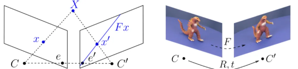
Thefundamental matrixFrepresents the map assigning a pointxin one image to the epipolar lineF xof possible matching points in the other image (see Fig.2.2, left). Such map is in fact a collineation (recall equation (1.9) in Section1.3.1). Since the really corresponding pointx0on that image lies on the epipolar lineF x, any matchx = (u, v)T _{↔ x}0 _{= (u}0_{, v}0₎T _{satisifies a constraint involving linearly}

F, called theepipolar constraint:

Epipolar Geometry and Fundamental Matrix 11

X

C

x

_x

F x

e

_e

C

Figure 2.2: Left: two cameras with centres C, C0_{, the epipoles e, e}0_{, a match}

x ↔ x0, and the epipolar line F x associated to an image point x. Right: The fundamental matrix contains information about the relative camera motion (2.14).

Although there are9coefficients forF in the previous equation, one parameter can be eliminated by removing the scale factor ambiguity inherent to the equation of a line (e.g. by takingF33= 1). Moreover, the image ofF is the set of epipolar lines, all passing through the epipolee0; therefore, the image of the collineation is not the whole set of lines of the plane, i.e. it has no full rank. Alternatively, this condition follows from the fact that, since the epipoles are in correspondence, the collineation is singular at the epipoles (F e=FT_e0 _{= 0). With little effort, the rank}

deficiency can be seen as equivalent to a rank two constrainton the fundamental matrixF:

detF = 0. (2.11)

Such additional constraint means that we need only7parameters to describe a fundamental matrix, i.e. F has 7 degrees of freedom. A possible (non-linear) minimal parameterisation for F consists in taking two rows as independent with one element being 1 (5 parameters in total), and then using two more parameters to write the third row as a linear combination of the two independent rows (note that 18 of such parameterisations would be required to describe all possible rank two

3×3matrices having an element equal to 1).

As in Section2.1.1for camera matrices, it can be observed that the epipolar constraint (2.10) is a projective map by nature. According to Section 1.3.1, by taking projective coordinates for the image matches,x = (u : v : 1),x0 = (u0 : v0 : 1), the epipolar constraint (2.10) reads simply

x0T_{F x= 0. (2.12)}

In particular, it follows thatFT _{is the fundamental matrix corresponding to the pair}

of images considered in reverse order.

As an example, let us deduce the expression of the fundamental matrix for a pair of camerasP0,P1as in (2.9). Concisely, imagine that we know the calibration matrices K, K0 of the pair of cameras, and the matrix Rof relative rotation and the vectortof relative translation between the camera frames, i.e. we know all the elements in (2.9). Then, any matching pairx↔x0 will by definition be the image of a 3D pointX; using projective coordinates for the image (x,x0being 3-vectors), this constraint becomesx 'P0(XT,1)T,x0 ' P1(XT,1)T. Then, by replacing

12 General Framework. Computer Vision Geometry

the camerasP0,P1with (2.9), we obtain

x'Kx , x0 'K0(RX+t). (2.13)

Finally, eliminatingXfrom the previous equations, one can deduce that any match-ing pair will satisfy the epipolar constraint (2.12) for the following fundamental matrix:

F ' (K0)−1T

[t]×RK−1. (2.14)

2.3.1 The (Normalised) Seven-Point Algorithm

In Chapter4, we will address the computation of a fundamental matrix given non-minimal sets of matches containing possibly noise and errors. However, we find convenient to benefit here from the fact that the epipolar constraint has been just in-troduced to explain into detail the fundamental matrix computation in the minimal case of 7 matches being given.

Assume as known 7 matchesxi = (ui, vi)T ↔x0i= (u0i, v0i)T,1≤i≤7, in a

general position. By considering the vector of unknowns

f = (F11, F12, F13, F21, F22, F23, F31, F32, F33)T , (2.15) each epipolar equation (2.10) reads:

aT_i ·f = 0, beingai = u u0, v u0, u0, u v0, v v0, v0, u, v,1

T

. (2.16)

Therefore, if we takeA:= (a1, . . . , a7)T, i.e. we stack the horizontal arraysaTi by

rows, we can build the following7×9linear system:

A·f = 0. (2.17)

We can then compute a basisf1,f2of the null-space ofA, and using (2.15) com-pute the associated matricesF1,F2. Finally, we can impose (2.11) to determine up to 3 solutionsF given by the real valuesλsolution of

F =λF1+ (1−λ)F2 , such that det(F) = 0. (2.18) Concisely, the equation det (λF1+ (1−λ)F2) = 0has degree 3 inλand thus it can have up to 3 real solutions.

Before applying the method described above, it is convenient to normalise the image coordinates for xi and x0i using respective transformations T and T0 that

send all points to a disk of radius √2centred at the origin; in this way, the coef-ficients of the corresponding f have all the same order and the matrixA is well conditioned [Har95]. Consequently, a straightforward denormalisation on the ob-tained solution needs to be performed at the end of the algorithm. The resulting method for the computation of the fundamental matrix given 7 point matches is known, and referred to from now on, as the normalised seven-point algorithm.

Epipolar Geometry and Fundamental Matrix 13

2.3.2 Matching Error Evaluation Using the Fundamental Matrix

Given a fundamental matrixF, the epipolar constraint (2.12) can be used to define different error measures of a potential match x ↔ x0 _{(recall Figure2.2). In this}

section, we denotex = (x1, x2,1)T,x0 = (x01, x02,1)T. Some of the errors below are represented in Figure2.3.

• Algebraic Error, the absolute error in the algebraic evaluation of (2.12):

a=|x0TF x|. (2.19)

• Geometric Error, the geometric distance fromx0_{to the epipolar lineF x:}

g1 = a q a2 x0 1 +a 2 x0 2 = |x 0T_{F x|} p (F x)2 1+ (F x)22 , (2.20)

whereaxi =∂a/∂xi, and(F x)iis the i-th coefficient of the lineF x.

• Symmetric Geometric Error, the average of the previous plus the geometric distance fromxto the epipolar lineFT_x0_:

g2 = 1 2   a p a2 x1 +a 2 x2 +_q a a2 x01+a 2 x02   . (2.21)

• Gold Standard Error, the the distance from the point(x1, x2, x01, x02)T to the quadric in those variables defined by the epipolar constraint (2.12):

G= min

ˆ

x,ˆx0

p

kx−xˆk2_+kx0_−xˆ0_k2_{subject toxˆ}0T_{Fxˆ= 0. (2.22)}

• Sampson Error, the first order approximation to the Gold Standard Error [TM97]: S = q a a2 x1 +a 2 x2 +a 2 x0 1+a 2 x0 2 . (2.23)

The Gold standard error cannot be computed in closed form: in [HS97] it was shown that it is equivalent to solving a univariate polynomial equation of degree

6; a fast accurate resolution was first proposed in [Kan96] and later improved in [KSN08]. The Sampson error [TM97] represents a first order approximation to the Gold Standard error and can be computed in closed form and as fast as the geometric error. Given a set of point matches, goodness-of-fit error measures for a fundamental matrix can be obtained by taking the average and/or Root Mean Square Error (RMSE) of the single-match measures above, the RMSE being the (uncorrected) sample standard deviation estimate.

14 General Framework. Computer Vision Geometry

Figure 2.3: Evaluation of a potential matchx ↔ x0 (in blue) givenF. The geo-metric error (2.20) corresponds to the point-line distance fromx0 to the epipolar lineF x. In red, the optimal matchxˆ ↔ xˆ0_{and associated epipolar lines (exactly}

passing through the points) corresponding to the Gold standard error (2.22).

2.3.3 A Numerical Example

Further than the theoretical computation of a fundamental matrix performed to deduce (2.14), we give next a (hopefully clarifying) numerical example of the epi-polar geometry concepts introduced so far. In order to ease the computations, we use normalised image coordinates, the pixel values being possibly non-integer or negative.

Consider the following matrix:

F =   0 0 0 1 0 √3 0 −1 0   . (2.24)

It has rank two, i.e. detF = 0, and thus it corresponds to a fundamental matrix. The coordinates of the epipoles can be computed as the nullspaces ofF andFT_:

e= (−√3 : 0 : 1), e0= (1 : 0 : 0). (2.25) Note that the epipoleelies inside the image, wherease0 _{represents the horizontal}

axis direction, rather than an image point. Since all epipolar lines pass through the epipole, in the second image all epipolar lines will be horizontal.

Consider the pair or image points(0,1)T _and(1,0)T_{, i.e.}

x= (0 : 1 : 1), x0 = (1 : 0 : 1). (2.26) The corresponding epipolar lines are:

FTx0 = (0 :−1 : 0), F x= (0 :√3 :−1), (2.27) meaning that the epipolar lines on the left and right image are, respectively:

{(u, v)T _{:v= 0}, {(u}0_{, v}0₎T _:v0 _{= 1/}√_3}

Applications of the Fundamental Matrix 15

See Figure2.3for a representation of the epipoles (2.25), the pair of points (2.26), and their epipolar lines (2.27), all in blue. The optimal exact matches in the sense of the Gold standard error (2.22), provided by the fast method of [KSN08], are

ˆ

x= (0.097 : 0.770 : 1), xˆ0 = (1.0 : 0.421 : 1). (2.29) See Figure2.3for a representation in red of these matches and their (exact) epipolar lines. The errors (2.19–2.23) from Section2.3.2are (using the notations therein):

a= 1.0, g1 = 0.577, g2= 0.789, G= 0.489, S = 0.5. (2.30) In general, the algebraic errorahas no geometric meaning and it should not be used for evaluation purposes.

2.4

Applications of the Fundamental Matrix

As we explained at the beginning of Chapter1, the fundamental matrix is a basic tool in Computer Vision. We conclude this chapter by outlining its main applica-tions, giving suitable references for the reader interested in further details.

2.4.1 Evaluating the Error in a Set of Matches

Given a set of matches, and a fundamental matrix, we can use the already explained measures in Section2.3.2to evaluate the matching error. See that section and the references therein for details.

2.4.2 Robust Matching

The error provided by a fundamental matrix can be used to classify an initial set of matches as inlier (correct) or outlier (wrong). Robust methods perform this classification without knowledge of the fundamental matrix, which is estimated as a byproduct of any robust method. In fact, robust matching is the main motivation of this work, and we are going to devote to it most of chapters4,5, and6.

2.4.3 Object Recognition

Robust matching can be used for object recognition as outlined in Chapter1. Sup-pose that we have the image of a query non-planar object, and that we are given a second image and we are asked to detect the instances of the query object in the new image. We can perform feature point detection on each image and then get an initial set of matches by using some intensity-based feature matching algorithm, which can be further refined with the help of the fundamental matrix geometry. In case of success in the latter robust matching step, the matches themselves give the location of the object in the second image. The presence of multiple instances of an object in an image is addressed by some of the robust methods (that we will review in this work), and the query against many images is addressed e.g. in [Low04,AZ12]. We will further explain this application in Chapter3.

16 General Framework. Computer Vision Geometry

PROJECTIVE AFFINE ”METRIC”

−→ −→

Figure 2.4: Stratified geometry for two images acquired by a pinhole camera.

2.4.4 3D Reconstruction and/or Camera Motion Estimation

Using a sparse set of matches between images of a static scene acquired by a moving camera, the scene and the camera motion (position and orientation) can be reconstructed with different ambiguity levels, depending on the knowledge, a priori or computed, on the cameras, the motion and the scene [HZ04]. Accord-ingly, the reconstructions may be calledprojective,affine, andmetricorEuclidean, which is commonly used for reconstructions with a similarity ambiguity. The re-covery of the camera motion in video sequences is also called visual odometry or visual localisation, and its simulataneous estimation with a 3D reconstruction in a video sequence is also known as SLAM (Simultaneous Localisation and Mapping) [DRMS07].

A projective reconstruction can be computed from the fundamental matrix [HZ04], which in turn can be computed given at least 7 general point matches between two images. The projective reconstruction can be upgraded to affine (resp. metric) if enough affine (resp. metric) scene, camera motion and/or cam-era calibration information is available (see Fig.2.4). Affine information is usually obtained by detecting sets of parallel directions (image vanishing points). The cam-era calibration is usually obtained with a calibration from pattern method exploit-ing known orthogonality relations on such pattern, although there exist alternative self-calibration approaches, not requiring any scene knowledge, as we explain next. The explicit computation of the camera motion given both a fundamental matrix and the camera calibration matrices will be needed in Section6.5, and consequently it will be previously explained into detail in Section6.4.3.

2.4.5 Camera Self-calibration

Camera self-calibration is an ambitious application domain that intends to determ-ine the camera calibration matrices, the camera motion, and the 3D reconstruction of a set of point matches, using as input solely the set of point matches. For in-stance, assuming fixed calibration matrices, three views are sufficient to solve the problem. See [HZ04] for a general overview on this area.

2.4.6 Dense Matching Via Image Rectification

Certain applications require a dense reconstruction of a scene or object, and thus a typically sparse set of features produced by SIFT or similar algorithms is not

Applications of the Fundamental Matrix 17

enough. In such context, the fundamental matrix (and the calibration matrix if available) can be used torectifythe images so that the epipolar lines are horizontal [HZ04], and then the search for a match requires only a 1D exploration inside a dis-parity range. The website http://vision.middlebury.edu/stereo/

contains a comprehensive enumeration and comparison of two-frame stereo cor-respondencealgorithms.

Chapter 3

Data Computation.

SIFT Detection and Matching

The Scale Invariant Feature Transform (SIFT) presented in [Low04] is invariant to image scale and rotation, and it has been shown to provide quite a robust matching across a substantial range of affine distortion, change in 3D viewpoint, addition of noise, and change in illumination. The features exploit classical ideas like corner detection and localisation refinement [HS88, FG87], and the scale-space theory as being formulated by Lindeberg in [Lin94,Lin98]. After introducing such ap-proaches, we present the SIFT feature and the detection and matching algorithms proposed in [Low04], as well as their performance limitations.

3.1

Harris Corner Detection and Sub-Pixel Refinement

Analytically, an edge will consist of points where the modulus of the gradient of the image (k∇Ik) is maximum, or, equivalently, the Laplacian of the image has a zero-crossing. Image corners instead can be characterised by the fact that there is a high variation in the gradient around the corner location. Therefore, the second-moment matrix∇I· ∇IT _{must have two ”strongly” non-zero eigenvalues.}

In practice, an image is a discrete two-dimensional signal with some inherent noise due to the characteristics of the used camera, the scene, and the acquisi-tion condiacquisi-tions. The image derivatives are computed using some finite difference approximation, after Gaussian smoothing is applied to the image (the direct estim-ation being too sensitive to noise). We denote byS thestructure tensor, which is defined at a pixel as the average over a local neighbourhood of the discrete second-moment matrix

∇I· ∇IT _{, (3.1)}

20 Data Computation. SIFT Detection and Matching

weighted by an isotropic Gaussian kernel.

The “approximate” rank of the structure tensorS characterises the local geo-metry of a pixel: the region is respectively uniform, and edge, or a corner, when the structure tensor is “close to” having rank 0, 1, or 2. If we denote by λ1, λ2 the eigenvalues ofS, it turns out thatdetS =λ1λ2,TrS =λ1+λ2. Harris and Stephens [HS88] compute the image corners as the local maxima of the function

detS −k(TrS)2 (3.2)

where k=0.06 is a positive (empirically adjusted) parameter. Such a measure is rotationally invariant and takes low values on edges or uniform regions. Many other measures have been proposed in the literature, see e.g. [Sze10].

Corner detection as described is inaccurate due to the use of smoothing (Gaus-sian) and finite approximation operators. A common practice is to refine the corner coordinates with sub-pixel accuracy. The F¨orstner algorithm [FG87] gives a re-fined location for a corner by computing the optimal intersection (in a least squares sense) of all tangent lines in a local neighbourhood of the detected corner. More details can be found in [Wik14a].

Both the computation of the image smoothing and gradient, and the structure tensor (or any local invariant) require the selection of spatial scale parameters, which will allow the detection of corners at the chosen scale but will miss other possible detections. This is the case, for instance, in an image containing both sharp corners and also rounded corners and diffuse corners. Although multi-scale operators exist, the introduction of the scale as a third inherent dimension has been shown to outperform such approaches.

3.2

Scale-Space

Lindeberg [Lin94] states that an internal representation is required to make cer-tain aspects of the image information content explicit and available to decision processes. Such representation is formed in the visual front-end and it should be independent of what can be expected to be in the scene. In particular, a multi-scale representation is the only reasonable approach. Moreover, it is natural to require that early visual operations are unaffected by certain primitive transformations, such as rigid motions of objects, illumination changes, changes in viewpoint or in object depths, etc.

Following Koenderink [Koe84], the requirements on an internal scale-space representation are:causality(“any feature at a coarse level of resolution is required to possess a (not necessarily unique) cause at a finer level of resolution although the reverse need not be true”),homogeneityandisotropy(i.e. all scale levels and spatial positions have equal importance). This formulation leads uniquely to the Gaussian kernel (and its derivatives) for generating the scale-space by convolution with the image. According to [Lin98], this is in agreement with neuro-physiological studies of biological evolution that have shown that there are receptive fields in the

mam-SIFT Features 21

malian retina and visual cortex, whose response profiles can be well modelled by Gaussian derivatives up to order four.

Explicitly, the scale-spaceL(x, y, σ)of an input imageI(x, y)is obtained by convolving it with a variable-scale GaussianG(x, y, σ):

L(x, y, σ) =G(x, y, σ)∗I(x, y), (3.3) where∗is the convolution (a.k.a. linear filtering) operator in(x, y), and

G(x, y) = 1 2πσ2e

−(x2_+y2_)/2σ2

. (3.4)

The Diference-of-Gaussian function convolved with the image [Low04], also termed Difference-of-Low-Pass [Lin94], is the difference of two nearby scales sep-arated by a constant factork:

D(x, y, σ) =L(x, y, kσ)−L(x, y, σ). (3.5) As shown in [Lin94] and reviewed by us in the next section, this function can be computed efficiently and it provides a close approximation to the scale-normalised Laplacian-of-Gaussian,σ2_∇2_{G, whenever a constant factorkrelates the different} scales. According to [Low04], detailed experimental comparisons performed by Mikolajczyk [Mik02] found that the extrema of this latter operator produce the most stable image features compared to a range of other possible image functions, including the aforementioned Harris corner function.

3.3

SIFT Features

TheScale Invariant Feature Transform (SIFT)feature descriptors [Low04] contain a keypoint with accurate scale-space coordinates, and an orientation parameter. The SIFT features contain moreover a4×4rotation-invariant descriptor that uses the histograms of directions (discretised to 8 values) around the keypoint location (4×4×8 = 128descriptor parameters).

3.3.1 SIFT Keypoints: Localisation

The scale-space (3.3) and the difference-of-Gaussians (3.5) are efficiently com-puted as follows. The initial image is first incrementally convolved with Gaussians separated by a constant factorkin scale space. The scale-space octaves (intervals between two consecutive powers of 2) are sequentially divided into s+ 2 inter-vals per octave for the convolved images and then sub-sampled. In other words, a Gaussian pyramid [Lin94] is built, in which the image size is successively (expo-nentially) reduced by a factor of2; this allows a great reduction in the computa-tional burden required to process the data. To avoid loosing high-frequency details when taking the Gaussian images, the original image is doubled in size using linear interpolation prior to building the pyramid.

22 Data Computation. SIFT Detection and Matching

The initial keypoint coordinates are detected as the local extrema in scale-space of the DoG pyramid. This ensures the scale-invariance of the feature localisation, and also its rotational invariance since these extrema are at the same time very close to the extrema of the Laplacian-of-Gaussian. The search for local extrema is performed efficiently by incrementally comparing each sample D(x, y, σ)with its 8 + 2 ×9 closest neighbours in the scale-space pyramid of DoG (rarely all neighbours need to be checked). The frequencies of sampling both in scale and space (the latter relative to the scale of smoothing) needed to obtain a maximal extrema detection stability are determined empirically. The highest repeatability is obtained when sampling 3 scales per octave; although repeatability increases with the value ofσ, a compromise w.r.t. efficiency is adopted by takingσ = 1.6.

The (spatial and scale) initial coordinates of each local extrema of the DoG pyr-amid are further refined using a quadratic approximation of the functionD(x, y, σ)

evaluated at the initial keypoint (finite difference approximations are used for the involved terms). The solution is determined by solving a3×3linear system. A minimum threshold of 0.3 is imposed on the absolute value ofDevaluated at a can-didate to extrema to accept it as such (assuming the image intensity in the range [0,1]).

Positive responses to edges are avoided by applying further a thresholdr = 10

on the ratio of principal curvatures. Similarly to the method by Harris (Section3.1) the Hessian matrix H is approximated at a candidate to corner, and its trace and determinant are used to avoid direct computation of its eigenvalues. Concisely, a candidate is accepted given that the HessianH=∇2_{Dat that candidate satisfies}

Tr(H) det(H) <

(r+ 1)2

r . (3.6)

3.3.2 SIFT Keypoints: Orientation

At the corresponding scale of each keypoint, an orientation is assigned as follows. First, image gradients are approximated using finite differences, then an histogram of gradient orientations (with 36 bins for the 360 degrees) is built in a local neigh-bourhood, where the orientations are weighted by the gradient module and by a Gaussian withσequal to 1.5 times the keypoint scale.

The peak in the histogram of orientations is assigned as orientation of the key-point, and any other local peak within a 80% of the highest peak frequency is used to create a new keypoint with that orientation. About a 15% of keypoints are re-ported to have multiple orientations assigned, but these contribute to the stability of matching.

The peak position is finally refined as the extrema of a parabola fitted to the 3 closest histogram bins. In this way, the angular resolution of the assigned orienta-tion is smaller than 10 degrees (the resoluorienta-tion of the built-up histogram). In fact, in an experimental evaluation with 40,000 keypoints, with 10% image noise, the orientation assignment was accurate on a 95% of the time, and in those cases the variance of orientation was shown to be less than 4 degrees [Low04].

SIFT Matching and Limitations 23

3.3.3 SIFT Descriptors

A local image descriptor is associated to a keypoint once its localisation and orient-ation have been assigned. The descriptor is a vector of 128 elements corresponding to a4×4grid of orientation histograms with 8 bins each. Such histograms are cre-ated as follows.

First, the keypoint scale is used to compute the orientation and magnitude of the gradient in a16×16quadrangular region with the orientation assigned to the keypoint around the keypoint spatial coordinates. Then, orientation histograms (8 bins each) over4×4sample regions are computed, weighting the gradient orienta-tions by the gradient magnitude weighted with a Gaussian window. By considering

4×4sample regions, the descriptor allows for shift in gradient positions: a gradi-ent sample on the left of a region can shift up to 4 sample positions while still contributing to the same histogram.

The purpose of using a weighting Gaussian window for the sampled gradients is to prevent sudden changes in the descriptor relative to small changes in location, and also to give a smaller weight to distant gradients that are more likely to be affected by registration errors. Trilinear interpolation is further used to distribute the value of each gradient sample into adjacent histogram bins. This operation is performed to avoid boundary effects, in which the descriptor changes abruptly when a sample shifts within an histogram or orientation.

Finally, two changes are performed on the descriptor to reduce the effects of illumination change on its performance. First, the descriptor is normalised to have norm one in order to allow affine changes in illumination (which at most produces a multiplicative change in gradient). Second, an empirically determined threshold of 0.2 is applied on the descriptor values, and the vector is then re-normalised. This intends to make the descriptor more robust against sudden changes in illumination by giving less preference to the magnitudes of large gradients in favour of the distribution of orientations.

3.4

SIFT Matching and Limitations

In the original paper [Low04], the SIFT features were used to identify a given query object or image inside an image database (object recognition). We next present the matching strategy that was developed accordingly, and outline the method limita-tions when applied to a pair of images.

3.4.1 Matching Algorithm

Two SIFT features are compared using the Euclidean distance between descriptors (vectors of 128 components explained in the previous section). However, given a feature in a query image, the selection of a matching feature in another image (possibly being part of an image database) is not based on an absolute threshold on the Euclidean distance between features, since this would make little sense given

24 Data Computation. SIFT Detection and Matching

104 Lowe

demonstrate their application, we will now give a brief description of their use for object recognition in the presence of clutter and occlusion. More details on ap-plications of these features to recognition are available in other papers (Lowe, 1999, 2001; Se et al., 2002).

Object recognition is performed by first matching each keypoint independently to the database of key-points extracted from training images. Many of these initial matches will be incorrect due to ambiguous fea-tures or feafea-tures that arise from background clutter. Therefore, clusters of at least 3 features are first identi-fied that agree on an object and its pose, as these clusters have a much higher probability of being correct than in-dividual feature matches. Then, each cluster is checked by performing a detailed geometric fit to the model, and the result is used to accept or reject the interpretation.

7.1. Keypoint Matching

The best candidate match for each keypoint is found by identifying its nearest neighbor in the database of keypoints from training images. The nearest neighbor is defined as the keypoint with minimum Euclidean distance for the invariant descriptor vector as was de-scribed in Section 6.

However, many features from an image will not have any correct match in the training database because they arise from background clutter or were not detected in the training images. Therefore, it would be useful to have a way to discard features that do not have any good match to the database. A global threshold on dis-tance to the closest feature does not perform well, as some descriptors are much more discriminative than others. A more effective measure is obtained by com-paring the distance of the closest neighbor to that of the second-closest neighbor. If there are multiple training images of the same object, then we define the second-closest neighbor as being the second-closest neighbor that is known to come from a different object than the first, such as by only using images known to contain different objects. This measure performs well because correct matches need to have the closest neighbor significantly closer than the closest incorrect match to achieve reli-able matching. For false matches, there will likely be a number of other false matches within similar distances due to the high dimensionality of the feature space. We can think of the second-closest match as provid-ing an estimate of the density of false matches within this portion of the feature space and at the same time identifying specific instances of feature ambiguity.

Figure 11. The probability that a match is correct can be deter-mined by taking the ratio of distance from the closest neighbor to the distance of the second closest. Using a database of 40,000 keypoints, the solid line shows the PDF of this ratio for correct matches, while the dotted line is for matches that were incorrect.

Figure 11 shows the value of this measure for real image data. The probability density functions for cor-rect and incorcor-rect matches are shown in terms of the ratio of closest to second-closest neighbors of each key-point. Matches for which the nearest neighbor was a correct match have a PDF that is centered at a much lower ratio than that for incorrect matches. For our ob-ject recognition implementation, we reob-ject all matches in which the distance ratio is greater than 0.8, which eliminates 90% of the false matches while discarding less than 5% of the correct matches. This figure was generated by matching images following random scale and orientation change, a depth rotation of 30 degrees, and addition of 2% image noise, against a database of 40,000 keypoints.

7.2. Efficient Nearest Neighbor Indexing

No algorithms are known that can identify the exact nearest neighbors of points in high dimensional spaces that are any more efficient than exhaustive search. Our keypoint descriptor has a 128-dimensional feature vector, and the best algorithms, such as the k-d tree (Friedman et al., 1977) provide no speedup over ex-haustive search for more than about 10 dimensional spaces. Therefore, we have used an approximate algo-rithm, called the Best-Bin-First (BBF) algorithm (Beis and Lowe, 1997). This is approximate in the sense that it returns the closest neighbor with high probability.

Figure 3.1: (Figure 11 in [Low04]) Empirical distributions for inliers (solid line) and outliers (dotted line). SIFT’s matching threshold 0.8 is a compromise.

the high variability between descriptors. Instead, the ratio of distances between the closest keypoint and the second closest one is deemed to be more effective.

The ratio criterion is based on the assumption that incorrect matches (outliers) will have several other matches at similar distances of the given keypoint given the high dimensionality of the feature space. The discriminative power of that measure has been validated empirically, and using simulation (Figure3.1) a threshold value of 0.8 has been determined to classify matches as correct (ratio closest/next closest below 0.8) or incorrect (otherwise).

For the object recognition task, a database of SIFT features was built, and then for the features in the query object an approximate search for the best and second best neighbours in the SIFT database was used (details in [Low04]). After a first search for objects having at least three matching features with the query object, a geometric test was performed to accept or reject the potential recognition. The exploitation of geometric constraints following a preliminary descriptor-based matching phase is a common practice and fits in the orientation of this work.

3.4.2 Limitations

The parameter selection in [Low04] is made using a synthetic database of 40,0000 keypoints. For generating such database, 32 real images were subject to controlled transformations, including rotation, scaling, affine stretch, change in brightness and contrast, and addition of image noise. Typical situations not modelled by such database are e.g. changes in viewpoint bigger than 50 degrees, anisotropic image noise, or repetitive patterns present in image textures.

The synthetic database was used to make initial decisions such as the fre-quency of sampling in scale (number of scales per octave) and in the spatial domain (amount of prior smoothing applied to each image level before building the octave), to select threshold values (used e.g. to reject unstable extrema in scale-space, to eliminate edge responses, to assign orientations, to tolerate sudden illumination changes), and many other decisions like the number of histograms, the number of bins per histogram, and the domain for each histogram.

A Case of Study (1/2) 25

A pair of real images not in that database will probably present different prop-erties (given the high dimensionality of a local patch) and thus the needed paramet-ers for that pair will probably differ from the original ones. Even worst, some of the SIFT parameters represent a compromise in some sense, and do not guarantee an optimal performance even for images in the original database. In conclusion, when given real images, incorrect matches are to be expected even if modifying the original SIFT parameters for feature detection and matching.

3.5

A Case of Study (1/2)

The website [Str08] contains image sequences used in the paper [SvV+08] to test the performance of different methods for multi-view stereo matching given all cam-era parameters. The provided calibration matrix, distortion parameters, and camcam-era pose were obtained using “on the ground” precise metric measurements taken at the time of acquisition; for this reason, we reffer to this calibration asground truth. We will use the first 6 images from the sequence calledCastle-P19(fourth on the site [Str08]), which contain an increasing amount of rotation among them, in such a way that between the first and the sixth image (see Fig. 3.2) there is a 90 degrees angular distance and little overlap. We consider half-size images, their size being1536×1024pixels. The ground truth epipolar geometry can be determined using (2.14) with the provided ground truth calibration, and taking into account the performed change in image size.

To exemplify the matching process, we first compute the SIFT features setting all the parameters as in the original paper [Low04]. The number of obtained SIFT features per image is quite high, as can be seen in the first column of Table 3.1. We also compute the matches between the first image and any other one, using the original threshold of 0.8, and also the thresholds 0.6 and 0.9. We will be interested in the accurate localisation coordinates of the matches, but not in their less accurate orientation. Therefore, the orientation is used in the matching process but discarded in the final data. Matches having the same coordinates are taken only once.

In Table3.1 we provide the obtained number of matches and an approximate value for the inlier ratio for the considered matching thresholds 0.6, 0.8, and 0.9. This approximate inlier ratio is computed by taking as inlier any point match with optimal geometric error (Section6.4.1), w.r.t. the ground truth fundamental matrix, below 3 pixels; this value is just a proxy for the inlier ratio (an unclear concept when dealing with real data) and it is not used for further evaluation.

As one could expect, by increasing the matching threshold the detected number of matches and the number of inliers increase; at the same time, the number of outliers increases even more and thus the inlier ratio decreases. It is to see in the continuation of this example in Section6.5.2which of the situations is more favourable for the estimation of the inlier matches and the fundamental matrix.

26 Data Computation. SIFT Detection and Matching

a) Castle-P19 im0 b) Castle-P19 im1

c) Castle-P19 im2 d) Castle-P19 im3

e) Castle-P19 im4 f) Castle-P19 im5

Figure 3.2: Six first images from Strecha’s Castle-P19 sequence [Str08].

Detection Matching (τ= 0.6) Matching (τ= 0.8) Matching (τ= 0.9) Image #SIFT #Match InRat* #Match InRat* #Match InRat*

im0 5908 im1 6235 1185 0.954 1780 0.833 2570 0.666 im2 7450 780 0.941 1289 0.780 2112 0.581 im3 7033 574 0.951 1025 0.789 1818 0.535 im4 6958 55 0.382 290 0.279 1070 0.147 im5 7355 20 0.350 260 0.188 1055 0.103 Table 3.1: SIFT detection and matching results for the Castle-P19 sequence. For each image we show the number of detected SIFT features in #SIFT. Then, we show the matching results for pairs containing the first image (im0), and using as thresholds τ for matching: the value τ = 0.8 as in the original paper, and

Chapter 4

Fundamental Matrix

Computation.

A Myriad of Methods

We will focus on the accurate computation of the fundamental matrix given a set of matches between 2D points. Other approaches exist considering matching re-gions or descriptors instead of points [MOC02,MCUP02,CMO04,PMC06]. For instance, in [GS08] only 2 SIFT matches are used at expense of precision (see Sec-tion 4 of the cited paper), since recall that while the SIFT key point localisaSec-tion is accurate, the rest of descriptors are assigned through processes consisting in voting from binned parameter space followed by interpolation.

A thorough introduction to the computation of a fundamental matrix from (point) matches can be found in [TM97], which we follow to some extent. A complimentary reference is [HZ04], although it dates back to 10 years ago. This fact, together with a lack of a complete review in the existing literature, motivates this chapter.

We will summarise the methods for computing a fundamental matrix from matching points. We will distinguish between methods designed to work for data containing only inliers and robust methods, the latter being able to return a list of inliers (correct matches) and the fundamental matrix. We will review in more de-tail the class of random sapling methods, that somehow started with the parametric RANSAC algorithm [FB81]. These methods randomly explore minimal sets of matches to hypothesise models, and some tolerate low inlier ratios (below 50%).

Recall that, according to Section 2.3, a fundamental matrix F = (Fij), 1 ≤

i, j ≤ 3, has rank two, its determinant being zero (2.11), and it is defined up to a scale ambiguity. In particular, 7 point matches allow to determine up to three fundamental matrices using the (normalised) seven-point algorithm, as explained in Section2.3.1.

28 Fundamental Matrix Computation. A Myriad of Methods

4.1

Methods for Inlier Data

In this section we assume givenninlier matchesxi ↔ x0i, withxi '(ui, vi,1)T,

x0_i '(u0_i, v0_i,1)T_{. The matches are correct but not exact, and the error distribution}

is not known, although its normality is a common assumption.

According to Section2.3, the estimation of the fundamental matrix using the given matches can be formulated as follows:

min F E F; xi, x0i subject to det(F) = 0, X F2 ij = 1, (4.1)

whereE(F;{xi, x0i})is an error function for the fundamental matrix that uses the

data matches.

The condition det(F) = 0 is non-convex, meaning that any local gradient method will possibly fall into a local minimum [BV10]; it can be imposed para-metrically, in which case the complexity of the cubic constraint disappears, but the parameterisation cannot be linear [BS04] and therefore it increases in turn the complexity of the error term making it non-convex. Moreover, more than one para-meterisations are needed to describe the set of fundamental matrices (recall e.g. the example in Section2.3), which usually suffer from artificial singularities [BS04]. The conditionP

F2

ij = 1can be replaced byF33 = 1or by any other constraint fixing the scale ambiguity inF.

The most commonly used error functions E in (4.1) are the sum of squared algebraic errors (2.19), Ealg F; xi, x0i := X i x0_iTF xi 2 , (4.2)

and the sum of squared geometric (2.20-2.21) or Sampson (2.23) distances; e.g. for the geometric error (2.20),

Egeom F; xi, x0i = X i x0T i F xi 2 (F xi)21+ (F xi)22 . (4.3)

The algebraic error formulation (4.2) is quite simple and allows closed form and fast resolution methods that we review below, although the rank two constraint on F cannot be handled in closed form. In fact, computing the fundamental mat-rix is a problem similar to fitting a conic (on a plane), for which minimising the algebraic error was known to be suboptimal and this motivated the use of geomet-ric (2.20) and Sampson (2.23) error formulations. The problem formulation using these errors is quite similar, and we will also review the related methods.

4.1.1 Algebraic Error Minimisation

Using the 9-vector f of unknowns defined by (2.15), and stacking by rows the epipolar constraints as in (2.16), we obtain a linear system like the one we built for 7 points in (2.17), its dimension being nown×9: