24
Appropriate Machine Learning Algorithm for Big Data
Processing
Emmanuel Boachie1 Prof Chunlin Li2
Wuhan University of Technology
School of Computer Science and Technology, Wuhan 430063, China
1Kumasi Technical University, Kumasi, Ghana
The work was supported by the National Natural Science Foundation (NSF) under grant (No.61472294, No.61672397)
Abstract
MLlib is Spark’s library of machine learning functions developed to operate in parallel on clusters. MLlib comprises of different types of learning algorithms and is available from all of Spark’s programming languages. Machine Learning is important to data scientists with a machine learning background considering using Spark, as well as engineers working with a machine learning professionals. A lot of algorithms in MLlib function better in terms of forecasting precision with regularization when that choice is accessible. Again, a lot of the SGDbased algorithms demand around 100 iterations to obtain good outcome. The paper presents the types of algorithms on distributed data sets, indicating all data as RDDs and recommends one which is more appropriate and effective for huge data processing. An assessment will be made based on their strength and weakness on the number of machine learning algorithms and come out with one which is effective for big data processing. The appropriate and effective machine learning algorithm is HashingTF as it takes the hash code of each word modulo a desired vector size, S, and thus maps each word to a number between 0 and S–1. This always provides an S-dimensional vector, and in practice is quite robust even if multiple words map to the same hash code. The MLlib inventors recommend setting S between 2 HashingTF can run either on one document at a time or on a whole RDD. It demands each “document” to be represented as an iterable order of objects for example, a list in Python or a Collection in Java.
Introduction
The philosophy and the design of MLlib are simple: it lets you invoke various algorithms on distributed data sets, standing for all data as RDDs. MLlib has come out with a few data types (e.g., tagged points and vectors), but at the end of it all, it is simply a set of functions to call on RDDs. Most algorithms in MLlib function better (in terms of prediction accuracy) with regularization when that option is accessible. Again, a lot of the SGDbased algorithms demand around 100 iterations to obtain good outcomes. MLlib attempts to offer valuable default values, but one should try to increase the number of iterations past the default to find out whether it enhances precision. For instance, with ALS, the default rank of 10 is fairly low, so one should try to increase this value. Make sure to evaluate these parameter changes on test data held out during training. MLlib introduces a few data types but at the end of it all, it is simply a set of functions to call on RDDs. MLlib attempts to provide valuable default values, but one should try to increase the number of iterations past the default to find out whether it enhances precision [1]
One important thing to note about MLlib is that it comprises only parallel algorithms that operate well on clusters. Some classic ML algorithms are not part because they were not developed for parallel platforms, but in contrast MLlib includes many recent research algorithms for clusters, such as distributed random forests, K-means||, and alternating least squares. This choice indicates that MLlib is appropriate for operating every algorithm on a large dataset. If we have many small datasets on which we want to train different learning models, it would be better to use a single- node learning library on every node, maybe calling it in parallel across nodes using a Spark map(). Similarly, it is common for machine learning pipelines to require training the same algorithm on a small dataset with many configurations of parameters, in order to select the best one. We can attain this in Spark by applying parallelize() over our list of parameters to train different ones on different nodes, again applying a single-node learning library on every node. But MLlib itself shines when we have a large, distributed dataset that we need to train a model on. [2]
Again, in Spark 1.0 and 1.1, MLlib’s interface is relatively low-level, giving us the functions to call for different jobs but not the higher-level workflow typically demanded for a learning pipeline (e.g., splitting the input into training and test data, or trying many combinations of parameters). In Spark 1.2, MLlib attains an additional (and at the time of writing still experimental) pipeline API for building such pipe lines.‐ This API look like higher-level libraries like SciKit-Learn, and will likely make it simple to write complete, self-tuning pipelines. Most algorithms in MLlib function better in terms of prediction accuracy with regularization when that choice is obtainable. Again, most of the SGDbased algorithms require around 100 iterations to obtain good outcomes. The is paper presents the algorithms types on distributed datasets, representing all data as RDDs and
25
recommend one which is more appropriate and effective for big data processing. The appropriate and effective machine learning algorithm is HashingTF as it takes the hash code of each word modulo a desired vector size, S, and thus maps each word to a number between 0 and S–1. This always provides an S-dimensional vector, and in practice is quite robust even if multiple words map to the same hash code. The MLlib developers recommend setting S between 2 HashingTF can run either on one document at a time or on a whole RDD. It requires each “document” to be represented as an iterable sequence of objects for instance, a list in Python or a Collection in Java. [3]
Related Work
The concept of Machine Learning is about learning from existing data to make predictions about the future. It is focused on creating models from input data sets for data-driven decision making.
Data science is the discipline of extracting the knowledge from huge datasets (structured or unstructured) to offer insights to business teams and influence the business strategies and roadmaps. The Data Scientist role is more serious than ever in addressing the challenges that are not easy to address applying the traditional numerical approaches. There are different types of machine learning models like Administered learning, Non-supervised learning, Partially-supervised Learning and Strengthening learning. Supervised learning: This method is applied to forecast a result by training the program applying an existing set of training data. Then the program is used to predict the label for a new unlabeled data set. [5]
Machine learning is the subfield of computer science that, according to Arthur Samuel in 1959, provides "computers the capacity to study without being clearly programmed."Evolved from the study of pattern recognition and computational learning theory in artificial intelligence,machine learning searches the study and creation of algorithms that can study from and give predictions on data. Such algorithms overcome following
strictly fixed program instructions by taking data-driven predictions or decisions, through developing a model from sample inputs. Machine learning is engaged in a range of computing jobs where designing and programming clear algorithms with good functionality is difficult or infeasible. For instance, applications which comprises email filtering, detection of network intruders or malicious insiders working towards a data breach, optical character recognition (OCR), learning to rank, and computer vision [11].
Machine learning is directly associated with computational statistics, which also emphases on prediction making through the computers usage. It has solid ties to mathematical optimization, which provides techniques, theory and application domains to the field. Machine learning is often conflated with data extraction, where the latter subfield emphases more on investigative data analysis and is termed as unsupervised learning. Machine learning can also be unsupervised and be applied to study and build baseline behavioral profiles for many entities and then applied to detect meaningful anomalies [12].
Considering the field of data analytics, machine learning is an approach applied to devise complex models and algorithms that lend themselves to prediction in commercial usage. This is known as projective analytics. These analytical models permit researchers, data scientists, engineers, and analysts to offer consistent, repeatable decisions and outcomes and expose hidden insights through studying from historical relationships and patterns in the data [13].
As of 2016, machine learning is a buzzword, and according to the Gartner hype cycle of 2016, at its peak of inflated expectations. Efficient machine learning is complex as discovering trends is difficult and regularly not sufficient training data is accessible. As a result, machine-learning programs often fails to achieve its objective.
There are two sub-models under administered machine learning, Regression and Classification.
Non-supervised learning: This is applied to identify hidden patterns and correlations within the raw
data. No training data used in this model, so this method is based on untagged data.
Algorithms such as k-means and Principle Component Analysis (PCA) fall into this category.
Partially-supervised Learning: This method applies both administered and non-supervised learning
models for predictive analytics. It adopts tagged and untagged datasets for training. It typically involves application of a small amount of branded data with a large amount of unbranded data. It can be used for machine learning approaches such as classification and regression.
Strengthening learning: The Strengthening Learning method is applied to learn how to expand a
numerical return objective by trying different actions and discovering which actions bring about the expanded return [6]
System Requirements
MLlib requires some linear algebra libraries to be installed on one`s machines. Firstly, one will need the gfortran runtime library for operating system. If MLlib warns that gfortran is missing, follow the setup instructions on the MLlib website. Secondly, to use MLlib in Python, we will need NumPy. If your Python installation does not have it (i.e., you cannot import numpy), the easiest way to get it is by installing the python-numpy or numpy
26
package through our package manager on Linux, or by using a third-party scientific Python installation like Anaconda. MLlib’s supported algorithms have also evolved over time [7]
Machine Learning Concept
Machine learning algorithms attempt to make predictions or decisions based on training data, often maximizing a mathematical objective about how the algorithm should behave. There are various kinds of learning problems, such as classification, regression, or clustering, which have different objectives. All learning algorithms require defining a set of elements for each item, which will be fed into the learning function. For instance, for an email, some components might comprise the server it comes from, or the number of mentions of the word free, or the color of the text. In many instances, defining the right elements is the most challenging part of applying machine learning. For instance, in a product recommendation task, simply adding another element. [8]
Most algorithms are defined only for numerical components (particularly, a vector of numbers representing the value for each feature), so often an important step is feature extraction and transformation to produce these feature vectors. For instance, for text classification (e.g., our spam versus non-spam case), there are several methods to featurize text, such as counting the frequency of every word. [9]
Once data is represented as feature vectors, most machine learning algorithms optimize a well-defined mathematical function based on these vectors. For instance, one classification algorithm might be to define the plane (in the space of feature vectors) that “best” separates the spam versus non-spam examples, according to some definition of “best” (e.g., the most points classified correctly by the plane). At the end, the algorithm will return a model representing the learning decision (e.g., the plane chosen). This model can now be applied to make projections on new points (e.g., see which side of the plane the feature vector for a new email falls on, in order to decide whether it’s spam)
Moreover, a lot of learning algorithms have multiple parameters that can affect outcomes, so real-world pipelines will train multiple versions of a model and calculate everyone. To perform this function, it is common to separate the input data into “training” and “test” sets, and train only on the former, so that the test set can be used to see whether the model overfit the training data. MLlib offers several algorithms for model evaluation. [10]
3. Methodology
a)The settings and Participants
Information needed for this research were gathered from the computer science department of Kumasi Technical University-Ghana. The rationale behind this is that the computer science lecturers in the department who are well versed on application of machine learning algorithms are the key instruments that can use the various machine learning algorithm to process big data which is growing in the departments and other functional sectors.
b) Data Collection
The researcher collected data from the computer science lecturers who were assigned to the task of using various machine learning algorithm to process data that increasing on daily basis in the computer science department. Others were also tasked to gather data from other functional sectors in the institution and use machine learning algorithm to process them.
c) Data Analysis
Data that were gathered from the various departments and other functional sections were considered for analysis. Qualitative approach was used for the analysis. The result enabled the researcher to study the true situation on the ground in terms of data mobilization and processing. This approach enabled the researcher to compare the strength and weakness of the various machine learning algorithm and recommend one which is more effective for big data processing
d) Quality Control Procedure
In order to ensure quality work as far as the implementation of Apache Spark; machine learning algorithm is concern, the computer science lecturers who are well versed in application of various algorithms to solve problems and have the ability to used mathematical formulas to explain certain concept were engaged. This enabled the researcher to come out with positive results.
4. Results
The findings of the research indicated that the appropriate and effective machine learning algorithm considered is HashingTF as it takes the hash code of each word modulo a desired vector size, S, and thus maps each word to a number between 0 and S–1. This always yields an S-dimensional vector, and in practice is quite robust even if multiple words map to the same hash code. The MLlib developers recommend setting S between 2 HashingTF can run either on one document at a time or on a whole RDD. It requires each “document” to be represented as an iterable sequence of objects for instance, a list in Python or a Collection in Java.
27
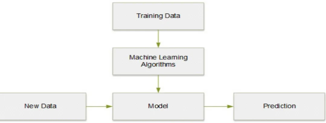
Machine Learning Process Flow
Figure 1 below shows the process flow of a typical machine learning solution.
Figure 1. Machine Learning Process Flow
It is imperative to ascertain that if the raw data is not cleaned or prepared before operating machine learning algorithms, the resulting patterns will not be precise or valuable as well as some anomalies may be missed. The quality of training data we provide to machine learning programs also plays a critical role in the prediction outcomes. If the training data is not random adequate, resulting patterns will not be precise. If the data is too small, the machine learning program may give inaccurate predictions
Discussions and Implications
In this section, we’ll cover the key algorithms available in MLlib, as well as their input and output types and also focus on how to call and configure these algorithms.
Feature Extraction
The mllib.feature package contains several classes for common feature transformations. These include algorithms to construct feature vectors from text (or from other tokens), and ways to normalize and scale features.
TF-IDF
The Term Frequency–Inverse Document Frequency, or TF-IDF, is a simple way to extract feature vectors from text documents (e.g., web pages). It computes two statistics for each term in each document: the term frequency (TF), which is the number of times the term happens in that document, and the inverse document frequency (IDF), which measures how (in)frequently a term happens across the whole document corpus. The product of these values, TF × IDF, indicates how relevant a term is to a specific document (i.e., if it is common in that document but rare in the whole corpus).
MLlib has two algorithms that compute TF-IDF: HashingTF and IDF, both in the mllib.feature package. HashingTF computes a term frequency vector of a given size from a document. In order to map terms to vector indices, it applies a technique called the hashing trick. Within a language like English, there are hundreds of thousands of words, so tracking a distinct mapping from every word to an index in the vector would be expensive. Instead, HashingTF picks the hash code of every word modulo a desired vector size, S, and thus maps every word to a number between 0 and S–1. This always provides an S-dimensional vector, and in practice is quite robust even if multiple words map to the same hash code. The MLlib developers recommend setting S between 2 HashingTF can run either on one document at a time or on a whole RDD. It requires each “document” to be represented as an iterable sequence of objects—for example, a list in Python or a Collection in Java.
Scaling
Most machine learning algorithms consider the magnitude of every component in the feature vector, and thus work best when the features are scaled so they weigh equally (e.g., all features have a mean of 0 and standard deviation of 1). Once you have built feature vectors, you can use the StandardScaler class in MLlib to do this scaling, both for the mean and the standard deviation. You create a StandardScaler, call fit() on a dataset to obtain a StandardScalerModel (i.e., compute the mean and variance of each column), and then call transform() on the model to scale a dataset.
28
Normalization
In some situations, normalizing vectors to length 1 is also useful to prepare input data. The Normalizer class permits this. Simply use Normalizer ().transform (rdd). By default Normalizer adopts the L norm (i.e, Euclidean length), but you can also pass a power p to Normalizer to use the L Word2Vec . Word2Vec is a featurization algorithm for text based on neural networks that can be adopted to feed data into many downstream algorithms. Spark includes an implementation of it in the mllib.feature.Word2Vec class. To train Word2Vec, you need to pass it a corpus of documents, represented as Iterables of Strings (one per word). Much like in “TF-IDF” menmapping them to lowercase and removing punctuation and numbers). Once you have trained the model (with Word2Vec.fit(rdd)), you will receive a Word2VecModel that can be adopted to trans form () each word into a vector. Note that the size of the models in Word2Vec will be equal to the number of words in your vocabulary times the size of a vector (by default, 100). You may wish to filter out words that are not in a standard dictionary to limit the size. In general, a good size for the vocabulary is 100,000 words.
Statistics
Basic statistics play an important role in data analysis, both in ad hoc exploration and understanding data for machine learning. MLlib provides several widely applied statistic functions that work directly on RDDs, via approaches in the mllib.stat.Statistics class. Some commonly adopted ones include: Statistics.colStats(rdd) Computes a statistical summary of an RDD of vectors, which stores the min, max, mean, and variance for each column in the set of vectors. This can be applied to get a wide variety of statistics in one pass. Statistics.corr(rdd, method). Computes the correlation matrix between columns in an RDD of vectors, applying either the Pearson or Spearman correlation (method must be one of pearson and spearman). Statistics.corr(rdd1, rdd2, method) Computes the correlation between two RDDs of floating-point values, adopting either the Pearson or Spearman correlation (method must be one of pearson and spearman). Statistics.chi SqTest(rdd) Computes Pearson’s independence test for every feature with the label on an RDD of LabeledPoint objects. Returns an array of ChiSqTestResult objects that capture the p-value, test statistic, and degrees of freedom for every feature. Label and feature values must be categorical (i.e., discrete values). Apart from these approaches, RDDs containing numeric data provide several basic statistics such as mean(), stdev(), and sum(), as described in “Numeric RDD Operations” . In addition, RDDs support sample() and sampleByKey() to build simple and stratified samples of data.
Classification and Regression
Classification and regression are two common forms of administered learning, where algorithms attempt to forecast a variable from features of entities using tagged training data (i.e., examples where we know the answer). The difference between them is the kind of variable predicted: in classification, the variable is discrete (i.e., it takes on a finite set of values termed classes); for example, classes might be spam or nonspam for emails, or the language in which the text is written. In regression, the variable predicted is continuous (e.g., the height of a person given her age and weight). Both classification and regression apply the LabeledPoint class in MLlib, mentioned in “Data Types” on page 218, mll pLab edP comprises simply of a label (which is always a Double value, but can be set to discrete integers for classification) and a features vector. For binary classification, MLlib expects the labels 0 and 1. In some texts, –1 and 1 are used instead, but this will lead to incorrect outcomes. For multiclass classification, MLlib expects labels from 0 to C–1, where C is the number of classes. MLlib includes a variety of approaches for classification and regression, including simple linear approaches and decision trees and forests.
Linear Regression
Linear regression is one of the most common methods for regression, forecasting the output variable as a linear combination of the features. MLlib also supports L and L regularized regression, commonly known as Lasso and ridge regression. The linear regression algorithms are accessible through the mllib.regression.Line arRegressionWithSGD, LassoWithSGD, and RidgeRegressionWithSGD classes. These follow a common naming pattern throughout MLlib, where problems involving multiple algorithms have a “With” part in the class name to specify the algorithm adopted. Here, SGD is Stochastic Gradient Descent.
These classes all have numerous parameters to tune the algorithm: numIterations Number of iterations to operate (default: 100). stepSize .Step size for gradient descent (default: 1.0). intercept Whether to add an interceptor bias feature to the data that is, another feature whose value is always 1 (default: false). regParam Regularization parameter for Lasso and ridge (default: 1.0). The way to call the algorithms differs slightly by language. In Java and Scala, you create a Linear Regression With SGD object, call setter approaches on it to set the parameters, and then call run() to train a model. In Python, you instead use the class method. Linear Regression With SGD .train(), to which you pass key/value parameters. In both cases, you pass in an RDD of Labeled Points,
29
Logistic Regression
Logistic regression is a binary classification method that identifies a linear separating plane between positive and negative examples. In ML lib, it takes Labeled Points with label 0 or 1 and returns a Logistic Regression Model that can predict new points. The logistic regression algorithm has a very similar API to linear regression. One difference is that there are two algorithms available for solving it: SGD and LBFGS. LBFGS is generally the best choice, but is not available in some earlier versions of MLlib (before Spark 1.2). These algorithms are available in the mllib. classification. Logistic Regression with LBFGS and With SGD classes, which have interfaces similar to Linear Regression with SGD. They take all the same parameters as linear regression.
The Logistic Regression Model from these algorithms computes a score between 0 and 1 for each point, as returned by the logistic function. It then returns either 0 or 1 depending on a threshold that can be set by the user: by default, if the score is at least 0.5, it will return 1. You can change this threshold via set Threshold(). You can also disable it altogether via clear Threshold(), in which case predict() will return the raw scores. For balanced datasets with about the same number of positive and negative examples, we recommend leaving the threshold at 0.5. For imbalanced datasets, you can increase the threshold to drive down the number of false positives (i.e., increase precision but decrease recall), or you can decrease the threshold to drive down the number of false negatives.
Support Vector Machines
Another binary classification method with linear separating planes are Support Vector Machines, or SVMs, expecting labels of 0 or 1. They are available through the SVMWithSGD class, with related parameters to linear and logisitic regression. The returned SVMModel uses a threshold for forecasting such as LogisticRegressionModel. Naive Bayes. Naive Bayes is a multiclass classification algorithm that scores how well each point belongs in each class depending on a linear function of the features. It is commonly applied in text classification with TF-IDF features, among other applications.
MLlib implements Multinomial Naive Bayes, which expects nonnegative frequencies (e.g., word frequencies) as input features. In MLlib, you can use Naive Bayes through the mllib.classification.NaiveBayes class. It supports one parameter, lambda (or lambda_ in Python), used for smoothing. You can call it on an RDD of LabeledPoints, where the labels are between 0 and C–1 for C classes. The returned NaiveBayesModel lets you predict() the class in which a point best belongs, as well as access the two parameters of the trained model: theta, the matrix of class probabilities for each feature (of size C × D for C classes and D features), and pi, the C-dimensional vector of class priors.
Decision Trees and Random Forests
The Decision trees are flexible model that can be applied for both classification and regression. They stand as a tree of nodes, each of which makes a binary decision based on a feature of the data and where the leaf nodes in the tree contain a prediction. Decision trees are attractive because the models are easy to inspect and because they support both categorical and continuous features. In MLlib, you can train trees using the mllib.tree.Decision Tree class, through the static methods train Classifier() and train Regressor(). Unlike in some of the other algorithms, the Java and Scala APIs also use static methods instead of a Decision Tree object with setters. The training methods take the following parameters: data, RDD of Labeled Point. Num Classes (classification only) Number of classes to use. Impurity, Node impurity measure; can be gini or entropy for classification, and must be variance for regression. Max Depth, Maximum depth of tree (default: 5). Max Bins, Number of bins to split data into when building each node (suggested value: 32). Categorical Features Info
A map specifying which features are categorical, and how many categories they each have. For example, if feature 1 is a binary feature with labels 0 and 1, and feature 2 is a three-valued feature with values 0, 1, and 2, you would pass {1: 2, 2: 3}. Use an empty map if no features are categorical. The online MLlib documentation contains a used. The cost of the algorithm scales linearly with the number of training examples, number of features, and max Bins. For large datasets, you may wish to lower max Bins to train a model faster, though this will also decrease quality. The train () methods return a Decision Tree Model. You can use it to predict values for a new feature vector or an RDD of vectors via predict(), or print the tree using to Debug String(). This object is serializable, so you can save it using Java Serialization and load it in another program.
Again, in Spark 1.2, MLlib adds an experimental Random Forest class in Java and Scala to build ensembles of trees, also known as random forests. It is available through Random Forest. Train Classifier and train Regressor. Apart from the per tree parameters just listed, Random Forest takes the following parameters: num Trees
How many trees to build. Increasing num Trees decreases the likelihood of over-fitting on training data. Feature Subset Strategy. Number of features to consider for splits at each node; can be auto (let the library select it), all, sqrt, log2, or one third; larger values are more expensive. Seed, Random-number seed to use. Random forests return a Weighted Ensemble Model that contains several trees (in the weak Hypotheses field, weighted by
30
weak Hypothesis Weights) and can predict() an RDD or Vector. It also includes a to Debug String to print all the trees.
Clustering
Clustering is the unsupervised learning task that involves grouping objects into clusters of high similarity. Unlike the supervised tasks seen before, where data is labeled, clustering can be used to make sense of unlabeled data. It is commonly used in data exploration (to find what a new dataset looks like) and in anomaly detection (to identify points that are far from any cluster).
K-means
K-means algorithm is considered in MLlib as popular for clustering, as well as a variant called K-means|| that offers better initialization in parallel atmospheres. K- means|| is similar to the K-means++ initialization procedure often applied in single- node settings. The most important parameter in K-means is a target number of clusters to generate, K. In practice, you rarely know the “true” number of clusters in advance, so the best practice is to try several values of K, until the average intracluster distance stops decreasing dramatically. Nevertheless, the algorithm picks only one K at a time. Apart from K, K-means in MLlib picks the following parameters: initialization Mode.
The method to initialize cluster centers, which can be either “k-means||” or “random”; k-means|| (the default) generally leads to better results but is slightly more expensive. MaxIterations, Maximum number of iterations to run (default: 100). runs Number of concurrent runs of the algorithm to execute. MLlib’s K-means supports operating from multiple starting positions concurrently and taking the best outcome, which is a good way to obtain a better overall model (as K-means runs can stop in local minima). Like other algorithms, you invoke K-means by creating a mllib.clustering.KMeans object (in Java/Scala) or calling KMeans.train (in Python). It takes an RDD of Vectors. K-means returns a K Means Model that lets you access the clusterCenters (as an array of vectors) or call predict() on a new vector to return its cluster. Note that predict() always returns the closest center to a point, even if the point is far from all clusters.
Collaborative Filtering and Recommendation
Collaborative filtering is a technique for recommender systems wherein users’ ratings and interactions with various products are used to recommend new ones. Collaborative filtering is attractive because it only needs to take in a list of user or product interactions: either “explicit” interactions or “implicit” ones. Based solely on these interactions, collaborative filtering algorithms study which products are similar to each other and which users are similar to each other, and can make new recommendations. While the MLlib API talks about “users” and “products,” you can also apply collaborative filtering for other applications, such as recommending users to follow on a social network, tags to add to an article, or songs to add to a radio station.
Alternating Least Squares
MLlib includes an implementation of Alternating Least Squares (ALS), a popular algorithm for collaborative filtering that scales well on clusters. It is located in the mllib.recommendation.ALS class. ALS works by determining a feature vector for each user and product, such that the dot product of a user’s vector and a product’s is close to their score. It takes the following parameters: rank Size of feature vectors to use; larger ranks can lead to better models but are more expensive to compute (default: 10). Iterations Number of iterations to run (default: 10) lambda Regularization parameter (default: 0.01). alpha. A constant applied for computing confidence in implicit ALS (default: 1.0). num User Blocks, num Product Blocks Number of blocks to divide user and product data in, to control parallelism; you can pass –1 to let MLlib automatically determine this (the default behavior). To use ALS, you need to give it an RDD of mllib. recommendation. Rating objects, each of which contains a user ID, a product ID, and a rating (either an explicit rating or implicit feedback). One challenge with the implementation is that each ID needs to be a 32-bit integer. If your IDs are strings or larger numbers, it is recommended to just use the hash code of each ID in ALS; even if two users or products map to the same ID, overall outcomes can still be good. Alternatively, you can broadcast() a table of product-ID-to-integer mappings to give them unique IDs. ALS returns a MatrixFactorizationModel representing its results, which can be used to predict() ratings for an RDD of (userID, productID) pairs.
Alternatively, you can apply model. Recommend Products(user Id, num Products) to find the top num Products() products recommended for a given user. Note that unlike other models in MLlib, the Matrix Factorization Model is large, holding one vector for each user and product. This means that it cannot be saved to disk and then loaded back in another run of your program. Instead, you can save the RDDs of feature vectors produced in it, model. User Features and model. Product Features, to a distributed filesystem.
Finally, there are two variants of ALS: for explicit ratings (the default) and for implicit ratings (which you enable by calling ALS.trainImplicit() instead of ALS.train()). With explicit ratings, each user’s rating for a
31
product needs to be a score (e.g., 1 to 5 stars), and the predicted ratings will be scores. With implicit feedback, each rating represents a confidence that users will interact with a given item (e.g., the rating might go up the more times a user visits a web page), and the predicted items will be confidence values.
Dimensionality Reduction Principal Component Analysis
Considering a dataset of points in a high-dimensional space, we are often interested in reducing the dimensionality of the points so that they can be analyzed with simpler tools. For instance, we might want to plot the points in two dimensions, or just reduce the number of features to train models more effectively. The main technique for dimensionality reduction adopted by the machine learning community is principal component analysis (PCA). In lower-dimensional space is done such that the variance of the data in the low- dimensional representation is maximized, thus ignoring noninformative dimensions. To compute the mapping, the normalized correlation matrix of the data is constructed and the singular vectors and values of this matrix are used. The singular vectors that correspond to the largest singular values are used to reconstruct a large fraction of the variance of the original data. PCA is currently available only in Java and Scala (as of MLlib 1.2). To invoke it, you must first represent your matrix using the mllib. linalg. distributed. RowMatrix class, which stores an RDD of Vectors, one per row.
Singular Value Decomposition
MLlib also offers the lower-level singular value decomposition (SVD) primitive. The SVD factorizes an m × n matrix A into three matrices A ≈ UΣV T, where:
• U is an orthonormal matrix, whose columns are called left singular vectors.
• Σ is a diagonal matrix with nonnegative diagonals in descending order, whose diagonals are called singular values.
• V is an orthonormal matrix, whose columns are called right singular vectors.For large matrices, usually we do not need the complete factorization but only the top singular values and its associated singular vectors. This can save storage, denoise, and recover the low-rank structure of the matrix. If we keep the top k singular values, then the dimensions of the resulting matrices will be U : m × k, Σ : k × k, and V : n × k . To achieve the decomposition, we call computeSVD on the RowMatrix class.
Model Evaluation
No matter what algorithm is used for a machine learning task, model assessment is a significant part of end-to-end machine learning pipelines. Many learning jobs can be tackled with different models, and even for the same algorithm, parameter settings can lead to different outcomes. Moreover, there is always a risk of overfitting a model to the training data, which you can best assess by testing the model on a different dataset than the training data. At the time of writing (for Spark 1.2), MLlib covers an experimental set of model evaluation functions, though only in Java and Scala. These are available in the mllib.evaluation package, in classes such as BinaryClassificationMetrics and MulticlassMetrics, depending on the problem. For these classes, you can create a Metrics object from an RDD of (prediction, ground truth) pairs, and then compute metrics such as precision, recall, and area under the receiver operating characteristic (ROC) curve. These methods should be run on a test dataset not used for training (e.g., by leaving out 20% of the data before training). You can apply your model to the test dataset in a map() function to build the RDD of (prediction, ground truth) pairs.
Algorithms Configurations
Most algorithms in MLlib perform better (in terms of prediction accuracy) with regularization when that choice is obtainable. Moreover, most of the SGDbased algorithms require around 100 iterations to obtain good outcomes. MLlib attempts to offer valuable default values, but you should try to increase the number of iterations past the default to see whether it enhances accuracy. For instance, with ALS, the default rank of 10 is fairly low, so you should try increasing this value. Make sure to assess these parameter changes on test data held out during training.
RDDs to Reuse
Most algorithms in MLlib are iterative, going over the data multiple times. Thus, it is vital to cache() your input datasets before passing them to MLlib. Even if your data does not fit in memory, try persist (Storage Level. DISK_ONLY In Python, MLlib automatically caches RDDs on the Java side when you pass them from Python, so there is no need to cache your Python RDDs unless you reuse them within your program. In Scala and Java, nevertheless, it is up to you to cache them.
32
Recognizing Sparsity
When your feature vectors contain mostly zeros, storing them in sparse format can result in huge time and space savings for big datasets. In terms of space, MLlib’s sparse representation is smaller than its dense one if at most two-thirds of the entries are nonzero. In terms of processing cost, sparse vectors are generally cheaper to compute on if at most 10% of the entries are nonzero. (This is because their representation demands more instructions per vector element than dense vectors.) But if going to a sparse representation is the difference between being able to cache your vectors in memory and not, you should consider a sparse representation even or denser data.
Level of Parallelism
For most algorithms, you should have at least as many partitions in your input RDD as the number of cores on your cluster to achieve full parallelism. Recall that Spark creates a partition for each “block” of a file by default, where a block is typically 64 MB. You can pass a minimum number of partitions to methods like SparkCon text.textFile() to change this, for example, sc.textFile("data.txt", 10). Alternatively, you can call repartition (numPartitions) on your RDD to partition it equally into numPartitions pieces. You can always see the number of partitions in each RDD on Spark’s web UI. At the same time, one must be careful with adding too many partitions, because this will increase the communication cost.
Pipeline API
Starting in Spark 1.2, MLlib is adding a new, higher-level API for machine learning, based on the concept of pipelines. This API is similar to the pipeline API in SciKit-Learn. In short, a pipeline is a series of algorithms (either feature transformation or model fitting) that transform a dataset. Each stage of the pipeline may have parameters (e.g., the number of iterations in LogisticRegression). The pipeline API can automatically search for the best set of parameters using a grid search, evaluating each set using an evaluation metric of choice. The pipeline API uses a uniform representation of datasets throughout, which is SchemaRDDs from Spark SQL. udifferent fields in the data. Various pipeline stages may add columns (e.g., a featurized version of the data). The overall concept is also similar to data frames in R. To give you a preview of this API, we include a version of the spam classification examples from augment the example to do a grid search over several values of the HashingTF and LogisticRegression parameters. [11]
6.2. Evaluation
Big data processing using machine learning algorithm can be evaluated under several criteria. Execution, Storage efficiency, generating effectiveness, and what it provides to the user are some of the criteria applied for assessment. The significance of these factors is by the system developer and the equally most appropriate machine learning procedure and data structure that will be designed for implementation are dependent on the decisions made by the developer.
The efficiency in its Execution is measured by the time it takes a module of the system or the system at large to perform a successful computation. It is measured using C supported systems. Execution efficiency is and always will be a major point of concern for big data processing systems.
6.3. Evaluation Environment
There is peer to peer kind of system architecture that have proved to be a better option to the tiresome and less flexible centralized system. The machine learning algorithm has adopted this type of network structure. There is not really a mother computer or machine that oversees others hence the named peer. All the computers in the machine learning domain are peers. This makes the transmission of information at any given time possible. Another benefit is that when some machines (computers) somewhere the domain malfunction, the others are likely to function irrespective to that. If this eventuality was to happen in a centralized kind of system, and the victim computer happens to be the main frame, the whole system will shut down and crumble. The peer to peer type of organization structure is convenient to sustain and faster in functionality compared to the main frame.
6.4 Data sources
Information that interests the team of researchers as the users of any data that comes from the computer science departments and few other functional sections in the Kumasi Technical University. They include text documents, sensor data, photographic pictures, biological sources, and web pages. Accessing this does require an intermediary which is common in the process of big data. The data to be processed is then carefully indexed for the later to be successful. This all process can be summarized as data mining in the data management system where information can be made available for decision making.
33
6.5 Parameter Setting
Parameter setting is a mode of attempting to generally and quickly clarify the language acquisition. It is simply a mode for processing massive data with machine learning algorithm to enhance continues performance of an institution. This idea offers accounts on why and how we are able to develop grammatically appropriate language in different instances without memorizing them. This is a typical instance in the large data processing applying machine learning algorithm.
A parameter set can be fitted to a different environmental setting through evolution simulation and the result is still hoped for by the consumer. To sum it up, parameter location makes it possible for the big data processing using machine learning algorithms to be an institutional based as the intranet which are the fastest route of communication is an institutional based web. It makes it efficient for information sharing to bypass language huddles and other impossible social standards. The most crucial part of parameter setting theory is to ascertain the kind of language provides enormous short-cuts. Compared to its effect in the big data processing with machine learning algorithm, the consumer does not really have to know the method he or she is adopting to get the information they are seeking for. That part has been encapsulated. The consumer only keys in his or her needs and a short while he gets them anywhere he or she is.
6.6 Metrics
Metrics is the calculation of performance of a given procedure. The metrics in big data are classified into categories. Online metrics calculate the original real-time users’ interactions with the exploration system. The offline metrics calculate the significance of the exploration engine via imposing expert moderators to calculate the probability of each outcome to suite the information needs of the consumer.
This metrics is estimated applying the set theory knowledge. It applies connections, cardinality symmetric distinction, summation etc. Online metrics is retrieved from data gathered from search logs. The Online metrics such as Click-through rate, session abandonment rate, session success rate, and zero outcome rate. The offline metrics is retrieved from vital ruling incidents. Here, judges are allowed to evaluate by score the effectiveness of each search result. Their score is in binary form meaning either superior or inferior no mediator or they apply a multilevel type of scale of satisfying unlimited search needs of the consumer.
The Normalized discounted collective gain is a metric that estimates the performance of a recommendation system based on the ranked significance of entities recommended. It ranks from 0.0 to 1.0. 1.0 stands for the grading of entities.
Parameters: p is the highest figure of entities advocated XYZp SXYZp is the highest
possible (ideal) XYZ for a given que of manuscripts cXYZP =
Conclusion
MLlib is Spark’s library of machine learning functions developed to operate in parallel on clusters. MLlib comprises of different types of learning algorithms and is available from all of Spark’s programming languages. Machine Learning is important to data scientists with a machine learning background considering using Spark, as well as engineers working with a machine learning professionals. A lot of algorithms in MLlib function better in terms of forecasting precision with regularization when that choice is accessible. Again, a lot of the SGDbased algorithms demand around 100 iterations to obtain good outcome. The is paper presents the algorithms types on distributed datasets, representing all data as RDDs and recommends one which is more appropriate and effective for big data processing. An experiment was embarked on based on their strength and weakness on the various machine learning algorithms at the selected functional sections in the above mentioned institution and come out with one which is more effective for big data processing. Here, lecturers at the computer science department who are well versed in the application were selected for the experimentation. The appropriate and effective machine learning algorithm is HashingTF according to the results of the experiment conducted. HashingTF takes the hash code of each word modulo a desired vector size, S, and thus maps each word to a number between 0 and S–1. This always provides an S-dimensional vector, and in practice is quite robust even if multiple words map to the same hash code. The MLlib inventors recommend setting S between 2 HashingTF can run either on one document at a time or on a whole RDD. It demands each “document” to be represented as an iterable order of objects for example, a list in Python or a Collection in Java.
Acknowledgment
The work was supported by the National Natural Science Foundation (NSF) under grant (No.61472294, No.61672397), Key Laboratory of Spatial Data Mining & Information Sharing of Ministry of Education, Fuzhou university (No. 2016LSDMISO5) program for the High-end Talents of Hubei Province Any opinions, findings,
34
and conclusions are those of the authors and do not necessarily reflect the views of the above agencies.
Reference
[1] Eduardo Z (2015) Spark vs Storm
[2] Srini P (2015) Big Data Processing using Apache Spark - Part 2: Spark SQL [3] Srini P (2015) Big Data Processing using Apache Spark - Part 3: Spark Streaming
[4] "Cluster Mode Overview - Spark 1.2.0 Documentation - Cluster Manager Types". apache.org. Apache Foundation. 2014-12-18. Retrieved 2015-01-18.
[5] "Spark Release 2.0.0". MLlib in R: SparkR now offers MLlib APIs [..] Python: PySpark now offers many more MLlib algorithms"
[6] Spark MLlib Programming Guide
[7] Spark Summit 2014 Machine Learning Training Exercise
[8] Penchikala .S (2014) Big Data Processing with Apache Spark - Part 4: Spark Machine Learning [9] Holden K et al (2015) “Learning Spark” Lightnin G-Fast Data Analysis
[10] "Spark Release 2.0.0". MLlib in R: SparkR.MLlib APIs [.] Python: PySpark now offers many more MLlib algorithms"
[11] Hu et al., “Collaborative Filtering for Implicit Feedback Datasets,” ICDM 2008 [12] Ron K; Foster Provost (1998). "Glossary of terms". Machine Learning. 30: 271–274.