Nonparametric Predictive Inference for System Reliability

Durham E-Theses

Nonparametric Predictive Inference for System

Reliability

ABOALKHAIR, AHMAD,MOHAMMAD,ABDALMONEM

How to cite:

ABOALKHAIR, AHMAD,MOHAMMAD,ABDALMONEM (2012) Nonparametric Predictive Inference for System Reliability, Durham theses, Durham University. Available at Durham E-Theses Online:

http://etheses.dur.ac.uk/3918/

Use policy

The full-text may be used and/or reproduced, and given to third parties in any format or medium, without prior permission or charge, for personal research or study, educational, or not-for-prot purposes provided that:

• a full bibliographic reference is made to the original source

• alinkis made to the metadata record in Durham E-Theses

• the full-text is not changed in any way

The full-text must not be sold in any format or medium without the formal permission of the copyright holders. Please consult thefull Durham E-Theses policyfor further details.

Academic Support Oce, Durham University, University Oce, Old Elvet, Durham DH1 3HP e-mail: [email protected] Tel: +44 0191 334 6107

http://etheses.dur.ac.uk

Nonparametric Predictive Inference for

System Reliability

Ahmad M. Aboalkhair

A thesis presented for the degree of

Doctor of Philosophy

Department of Mathematical Sciences

University of Durham

England

May 2012

Dedicated

To my father

Who has been a great source of motivation and endless support in my life Thank you for all your sacrifices for me to help me become what I am now

To the soul of my mother

For all unlimited love, sacrifices, inspiration, prayers and faith in me I wish I could kiss her hand and tell her how much I appreciate that

To my wife

For her endless love, support, encouragement and belief in me Thank you for being there during the hardest of times

To my lovely children

for lighting up my life with their smile

To my brothers and sisters

Nonparametric Predictive Inference for

System Reliability

Ahmad M. Aboalkhair

Submitted for the degree of Doctor of Philosophy

May 2012

Abstract

This thesis provides a new method for statistical inference on system reliability on the basis of limited information resulting from component testing. This method is called Nonparametric Predictive Inference (NPI). We present NPI for system reliability, in particular NPI fork-out-of-msystems, and for systems that consist of multipleki_-out-of-mi _{subsystems in series configuration. The algorithm for optimal}

redundancy allocation, with additional components added to subsystems one at a time is presented. We also illustrate redundancy allocation for the same system in case the costs of additional components differ per subsystem.

Then NPI is presented for system reliability in a similar setting, but with all subsystems consisting of the same single type of component. As a further step in the development of NPI for system reliability, where more general system structures can be considered, nonparametric predictive inference for reliability of voting sys-tems with multiple component types is presented. We start with a single voting system with multiple component types, then we extend to a series configuration of voting subsystems with multiple component types. Throughout this thesis we assume information from tests ofnt components of type t.

Declaration

The work in this thesis is based on research carried out at the Department of Mathe-matical Sciences, Durham University, UK. No part of this thesis has been submitted elsewhere for any other degree or qualification and it is all the author’s original work unless referenced to the contrary in the text.

Copyright © 2012 by Ahmad M. Aboalkhair.

“The copyright of this thesis rests with the author. No quotations from it should be published without the author’s prior written consent and information derived from it should be acknowledged”.

Acknowledgements

First and foremost, all thanks and praise to Allah Almighty for his countless blessings he has bestowed on me generally and in accomplishing this thesis especially.

I would like to express my deepest gratitude to my supervisor Prof. Frank Coolen. To work with him is a real pleasure to me. He is always patient and en-couraging in times of new ideas and difficulties. He listens to my ideas and discus-sions with him frequently lead to key insights. His ability to select and to approach compelling research problems, his high scientific standards, and his hard work set an example. I admire his ability to balance research interests and personal pursuits. Above all, he made me feel a friend, which I appreciate from my heart. It is very hard to find the words to express my appreciation for him. Actually, without his help and guidance this work would not have been possible.

I would like also to express my immense gratitude to my second supervisor, Dr. Iain MacPhee. To my great sadness, Iain MacPhee passed away in January 2012 following a long standing battle with cancer. He was an excellent supervisor. He patiently taught me so much that has enriched my knowledge, and I wish I could tell him how much I appreciate that.

My final thanks go to everyone who has assisted me, stood by me or contributed to my educational progress in any way.

Contents

1.2 Nonparametric predictive inference . . . 3

1.3 k-out-of-m systems . . . 4

1.4 Outline of thesis . . . 8

2 Series of independent voting subsystems 10 2.1 Introduction . . . 10

2.2 NPI for Bernoulli quantities . . . 11

2.3 NPI for a k-out-of-m system . . . 14

2.3.1 Examples ofk-out-of-m systems . . . 16

2.4 Series of independent ki_-out-of-mi _{subsystems . . . 18}

2.5 Redundancy allocation . . . 22

2.5.1 Redundancy allocation algorithm . . . 22

2.5.2 Optimality of redundancy allocation algorithm . . . 24

2.6 Redundancy allocation with component costs . . . 29

2.7 Concluding remarks . . . 32

3 Subsystems consisting of one type of component 34 3.1 Introduction . . . 34

Contents vii

3.2 Series of subsystems consisting of single-type components . . . 35

3.2.1 Two subsystems . . . 35

3.2.2 L≥2 subsystems . . . 37

3.3 Examples . . . 39

3.4 Concluding remarks . . . 47

4 Voting systems with multiple component types 48 4.1 Introduction . . . 48

4.2 Multiple component types . . . 50

4.2.1 System description . . . 50

4.2.2 NPI lower and upper probabilities for functioning of the system 51 4.2.3 Derivation of the NPI lower and upper probabilities for func-tioning of the system . . . 53

4.2.4 Redundancy allocation . . . 55

4.3 Examples . . . 57

4.4 Concluding remarks . . . 64

5 Subsystems with multiple component types 66 5.1 Introduction . . . 66

5.2 Subsystems with multiple component types . . . 67

5.3 2 subsystems with 2 component types . . . 69

5.4 L subsystems with T component types . . . 70

5.5 Examples . . . 77

5.6 Concluding remarks . . . 81

6 Conclusions 83

Appendix 89

A Brief guide to notation 89

Chapter 1

Introduction

In classical reliability theory most of the methods and models use precise probabili-ties to quantify uncertainty, assuming completeness of the probabilistic information about the system and component reliability behaviour. Walley [57] discussed many reasons why precise probability is too restrictive for practical uncertainty quantifi-cation. In reliability, the most important ones include limited knowledge and infor-mation about random quantities of interest, and possibly inforinfor-mation from several sources which might appear to be conflicting if restricted to precise probabilities.

During the past few decades, several alternative methods for uncertainty quan-tification have been proposed, some also for reliability. For example, fuzzy reliability theory [11] and possibility theory [32] provided solutions to problems that could not be solved satisfactorily with precise probabilities. The theory of imprecise probabil-ities [57] and the theory of interval probability [59] have been used as a general and promising tool for reliability analysis. Coolen [13] provided an insight into impre-cise reliability, discussing a variety of issues and reviewing suggested applications of imprecise probabilities in reliability, see [54] for a detailed overview of imprecise reliability and many references.

In this thesis a statistical approach which uses imprecise probability is presented for system reliability. This approach is called Nonparametric Predictive Inference (NPI). It provides a new method for statistical inference on system reliability on the basis of limited information resulting from component testing.

1.1. Imprecise probability 2

Section 1.1 provides a brief introduction to imprecise probability, which is an umbrella term encompassing all qualitative and quantitative ways of measuring un-certainty without single-valued probabilities. In Section 1.2 we review briefly the main idea of NPI. The class of k-out-of-m systems and a brief overview of some recent contributions that focus on reliability of this class of systems is presented in Section 1.3. The outline of this thesis is given in Section 1.4.

1.1

Imprecise probability

The idea to use interval-valued probabilities dates back at least to the middle of the nineteenth century [10]. In recent years this has particularly been a growing area of research. Researchers with widely varying backgrounds are currently contributing to theory, and indeed applications, of imprecise probability, including mathemati-cians, statistimathemati-cians, computer scientists, and researchers working on artificial intel-ligence, medicine, and a variety of engineering areas. Such researchers are brought together via the Society for Imprecise Probability Theory and Applications (SIPTA,

http://www.sipta.org), which also organizes biennial conferences.

In classical probability theory, a single probability P(A) ∈ [0,1] is used to quantify uncertainty about an event A. Lower and upper probabilities general-ize the standard theory of (‘single-valued’ or ‘precise’) probability and provide a powerful method for uncertainty quantification [54]. The main idea is that, for an event A, lower probability P(A) ∈ [0,1] and upper probability P(A) ∈ [0,1] with 0≤ P(A)≤ P(A)≤ 1 are specified, such that these lower and upper probabilities define a so-called ‘structure’ M, which is a set of precise probability distributions corresponding to the lower and upper probabilities in the sense that for each prob-ability distribution P(·) ∈ M, P(A) ≤ P(A) ≤ P(A) and P(A) = infP(·)∈MP(A)

andP(A) = sup_P(·)∈MP(A) [8]. The classical situation of precise probability occurs if P(A) = P(A), whereas P(A) = 0 and P(A) = 1 represents complete lack of knowledge aboutA. These lower and upper probabilities are naturally linked by the conjugacy propertyP(A) = 1−P(Ac_{) [8]. This generalization allows indeterminacy}

1.2. Nonparametric predictive inference 3

interpreted in several ways. One can consider them as bounds for a precise proba-bility, related to relative frequency of the eventA, reflecting the limited information one has about A. Generally, P(A) reflects the information and beliefs in favour of event A, whileP(A) reflects such information and beliefs against A, so in favour of Ac_.

Coolen [12] presented lower and upper predictive probabilities for Bernoulli ran-dom quantities. These lower and upper probabilities are part of a wider statistical methodology called ‘Nonparametric Predictive Inference’ (NPI), which is a frequen-tist stafrequen-tistical approach with strong consistency properties in the theory of imprecise probability [8].

1.2

Nonparametric predictive inference

Nonparametric predictive inference (NPI) is a statistical method to learn from data in the absence of prior knowledge and using only few modelling assumptions. It provides a solution to some explicit goals for objective (Bayesian) inference, for example the empirical and logical norms as formulated by Williamson [60]. These goals cannot be obtained when using precise probabilities, but are achieved by NPI after slight reformulation to allow the use of lower and upper probabilities [14]. It is also exactly calibrated [39], which is a strong consistency property in frequentist statistics, and it never leads to results that are in conflict with inferences based on empirical probabilities.

NPI is based on Hill’s assumption A(n) [35], which gives direct probabilities [31]

for a future observable random quantity, based on observed values of n related random quantities. Suppose thatX1,· · · , Xn, Xn+1are continuous and exchangeable

random quantities. So, for one such a random quantity, its rank among all these random quantities is uniformly distributed over the values 1 ton+ 1 (assuming no ties for simplicity). Let the ordered observed values of X1,· · · , Xn be denoted by

x(1) < x(2) <· · ·< x(n) <1, and letx(0) =−∞andx(n+1) =∞for ease of notation.

For a future observationXn+1, based on n observations, A(n) is

P (Xn+1 ∈(xj−1, xj)) =

1

1.3. k-out-of-m systems 4

A(n) does not assume anything else, and can be considered to be a post-data

as-sumption related to exchangeability [30]. For a detailed discussion of A(n) we refer

to Hill [36]. Inferences based onA(n)are predictive and nonparametric, and are

suit-able if there is hardly any knowledge about the random quantity of interest, other than the first n observations, or if one does not want to use such information, for example to study effects of additional assumptions underlying other statistical meth-ods. Nevertheless,A(n) has not received much attention in the statistical literature.

A logical reason is that it only assigns equal probabilities for the next observation to belong to each of then+ 1 intervals created by the previousn observations, so very few inferences can be based on this without requiring additional assumptions. How-ever, it provides bounds for probabilities for all events of interest involving Xn+1.

These bounds follow from De Finetti’s fundmental theorem of probability [30] and are the sharpest bounds for all events, corresponding to the probabilities defined by the assumption A(n). Consequently, these are lower and upper probabilities in the

theory of imprecise probability.

NPI is a framework of statistical theory and methods that use these A(n)-based

lower and upper probabilities. It has been presented for Bernoulli data [12], real-valued data [8], data including right-censored observations [25] and multinomial data [21,22]. NPI has a wide range of applications in statistics, operational research and reliability [17]. For example, applications of NPI to basic problems in reliability include reliability demonstration for failure-free periods [23], (opportunity-based) age replacement [26, 27], comparison of success-failure data [28], probabilistic safety assessment in case of zero failures [15], and prediction of not yet observed failure modes [16]. In this thesis, we are interested in NPI for system reliability, in particular NPI for k-out-of-m systems, and for systems that consist of multiple ki_-out-of-mi

subsystems in series configuration [18, 19, 42].

1.3

k

-out-of-

m

systems

The class of k-out-of-m systems, also called ‘voting systems’, was introduced by Birnbaum [9]. These are systems that consist ofmexchangeable components (often

1.3. k-out-of-m systems 5

the confusing term identical components is used), such that the system functions if and only if at least k of its components function. Since the value of m is usually larger than the value of k, redundancy is generally built into a k-out-of-m system. Both parallel and series systems are special cases of thek-out-of-msystem. A series system is equivalent to an m-out-of-m system while a parallel system is equivalent to an 1-out-of-m system.

Throughout this thesis, we use the term ‘exchangeable components’ to indicate the scenario required for application of A(n) as described in Sections 1.2 and 2.2.

Effectively, exchangeable components are ‘similar’ with regard to our knowledge about their functioning. In practice, this may typically apply to components which are manufactured in the same process and which have similar roles in the system which is being considered. Information about the quality of components is assumed to come from testing of further components which are exchangeable with those in the system. Therefore, this would typically require that tests take place under similar circumstances as will apply to the functioning of the components in the system.

Applications ofk-out-of-msystems can e.g. be found in the areas of target detec-tion, communicadetec-tion, safety monitoring systems, and, particularly, voting systems. The k-out-of-m systems are a very common type in fault-tolerant systems with re-dundancy. They have many applications in both industrial and military systems. Fault-tolerant systems include the display system in a cockpit, the multi-engine system in an airplane, and the multi-pump system in a hydraulic control system [52]. For example, a car with aV8 engine may be driven if only four cylin-ders are firing. But, if less than four cylincylin-ders fire, then the car cannot be driven. Thus, the functioning of the engine can be considered as a 4-out-of-8 system. The system is tolerant of failures of up to four cylinders for minimal functioning of the en-gine [38]. In a data processing system with five video displays, a minimum of three displays operable may be sufficient for full data display. In this case the display system functions as a 3-out-of-5 system. In a communications system with three transmitters, the average message load may be such that at least two transmitters must be operational at all times, or else critical messages may be lost. Thus, the transmission system behaves as a 2-out-of-3 system. Systems with spares may also

1.3. k-out-of-m systems 6

be represented by a k-out-of-m system model. A car with four tires, for example, usually has one additional spare tire. Thus, the vehicle can be driven as long as at least 4-out-of-5 tires are in good condition [38].

A traditional problem considered in reliability theory is assessment of system reliability [7], where voting systems have received particular attention. Many recent contributions to the literature focus on reliability of the class ofk-out-of-msystems, albeit from a classical perspective using precise probabilities to quantify uncertainty. For example, Torres-Echeverria et al. [53] address modelling of probability of dan-gerous failure on demand and spurious trip rate of safety instrumented systems that includek-out-of-mvoting redundancies in their architecture. Senz-de-Cabezn et al.

[49] presented computational algebraic algorithms for the reliability of generalized k-out-of-mand related systems. They analysed and computed identities and bounds for the reliability of coherent systems using the techniques of commutative algebra. They applied the techniques to the analysis of some of the most relevantk-out-of-m systems. They concluded that the efficiency of their approach in obtaining exact identities, bounds and asymptotic formulas shows good performance when compared with others results from the literature.

Moghaddass et al. [45] consider a general repairable k-out-of-m system with non-identical components that can have different repair priorities. They address the problem of efficient evaluation of the system’s availability in a way that steady state solutions can be obtained systematically with reasonable computation time. Vaurio [56] considers the unavailability of redundant standby systems with k-out-of-mlogic. Such systems are subject to latent failures that are detected by periodic tests and repaired immediately after discovery. He considers many potential failure and error modes in the formalism, evaluates both consecutive and staggered testing schemes and suggests methods for including common cause failures in the analyses. Levitin [40] proposes a model that generalizes linear consecutive k-out-of-r-from-m systems to linear n-gap-consecutive k-out-of-r-from-m : F systems. In this model the system consists ofmlinearly ordered statistically independent identical elements and fails if the gap between any pair of groups ofr consecutive elements containing at leastk failed elements is less than n elements.

1.3. k-out-of-m systems 7

Erylmaz [33] studied circular consecutive k-out-of-m systems consisting of ex-changeable components. He derived explicit expressions for both unconditional and conditional survival functions for 2k+ 1≥m, while signature-based mixture repre-sentations for generalkare obtained. Salehiet al.[50] considered linear and circular consecutive k-out-of-m systems. It is assumed that lifetimes of components of the systems are independent but their probability distributions are non-identical. The reliability properties of the residual lifetimes of such systems under the condition that at leastm−r+1, withr≤m, components of the system are operating was stud-ied. The probability that a specific number of components of the above-mentioned system operate at time t, t > 0, under the condition that the system is alive at time t was also investigated. Gurler and Capar [34] established an algorithm for the computation of the mean residual lifetime of an (m−k+ 1)-out-of-m system in the case of independent but not necessarily identically distributed lifetimes of the components. They gave an application for the exponentiated Weibull distribution to study the effect of various parameters on the mean residual lifetime of the sys-tem. The relationship between the mean residual lifetime for the system and that of its components was also investigated. Ruiz-Castro and Li [48] presented an algo-rithm for a general discrete voting system subject to several types of failure with an indefinite number of repairpersons. The model is built and the stationary distribu-tion, for the general case, is derived using matrix-analytic methods. They computed performance measures of interest for the transient and the stationary regime, includ-ing availability, reliability and the conditional probability of failure for the different types of failures and for the system.

These recent papers are evidence of the continuing importance of development of methodology to quantify system reliability. The NPI approach presented in this thesis provides the important opportunity to reflect, by the use of lower and upper probabilities, the fact that information from tests is often quite limited.

1.4. Outline of thesis 8

1.4

Outline of thesis

In this thesis, we present important extensions for the NPI approach to system re-liability. Coolen-Schrijner et al. [29] considered NPI for system reliability, and in particular for series systems with subsystemiaki_-out-of-mi_{system. They presented}

an attractive algorithm for optimal redundancy allocation, with additional compo-nents added to subsystems one at a time. However, they only proved this result for test data with no failed components. We start with generalising the algorithm for redundancy allocation presented by Coolen-Schrijner et al. [29] to general test results, a situation in which redundancy plays an even more important role than when testing revealed no failures at all. We also illustrate redundancy allocation for the same system in case the costs of additional components differ per subsystem. Then NPI is presented for system reliability in a similar setting, but with all sub-systems consisting of the same single type of component. As a further step in the development of NPI for system reliability, where more general system structures can be considered, nonparametric predictive inference for reliability of voting systems with multiple component types is presented. We start with a single voting system with multiple component types, then we extend to a series configuration of voting subsystems with multiple component types. Throughout this thesis we assume in-formation from tests ofnt components of typet. All computations were performed

using R. Some parts of this thesis have been presented at conferences and related papers have been published in academic journals or are in submission [1–6,18,19,42]. Chapter 2 begins with a brief overview of NPI for Bernoulli data, using a path counting technique to compute upper and lower probabilities. We present the main results on NPI fork-out-of-msystems, and these results are illustrated and discussed via examples. We provide a detailed presentation of optimal redundancy allocation following general component test results and the proofs of the main results. We present another extension for the NPI approach to system reliability, namely inclu-sion of different costs per component of the different types. Part of this chapter was presented at the 18th Advances in Risk and Reliability Technology Symposium (Loughborough, UK, 2009) [1].

1.4. Outline of thesis 9

In Chapter 3, we consider NPI for system reliability in a similar setting, but with all subsystems consisting of the same single type of component. Such components are exchangeable with regard to the information about them contained in test results but they play different roles in the system if they are in different subsystems. NPI lower and upper probabilities for a series of twoki_-out-of-mi _{subsystems consisting}

of single-type components are derived. These results are generalized to systems with L ≥ 2 ki_-out-of-mi _{subsystems in a series configuration. This chapter was}

presented (by Frank Coolen) at a symposium in remembrance of Professor Jan M. van Noortwijk (Delft, the Netherlands, 2009) [18].

In Chapter 4, we consider more general system structures. Whilst restricting attention to a single voting system, this can now consist of multiple types of com-ponents. They are assumed to all play the same role within the system, but with regard to their reliability components of different types are assumed to be indepen-dent. This chapter was presented at the International Conference on Accelerated Life Testing, Reliability-based Analysis and Design: ALT2010 (Clermont-Ferrand, France, 2010) [2].

In Chapter 5, we generalize the results introduced in Chapters 2, 3 and 4 by considering systems in series structure where each subsystem is a voting system with multiple types of components and with components of the same type appearing in different subsystems. A part of Chapter 5 was presented at the 19th Advances in Risk and Reliability Technology Symposium (Stratford-upon-Avon, UK, 2011) [3], and a comprehensive overview of Chapter 5 and the main parts of this thesis was presented at the European Safety & Reliability Conference - ESREL 2011 (Troyes, France, 2011) [4].

In Chapter 6, we discuss opportunities to extend the research presented in this thesis, which is also discussed in the final sections of each of Chapters 2 to 5.

Although the most general results in Chapter 5 contain the results of Chapters 2, 3 and 4 as special cases, the presentation in this thesis reflects the progress of the research project over time and in every step a substantial problem is solved, hence this order of detailed presentation provides much insight into the complexities involved.

Chapter 2

Series of independent voting

subsystems

2.1

Introduction

Coolen-Schrijner et al. [29] considered NPI for system reliability, and in particular for series systems with subsystem i a ki_-out-of-mi _{system. Such systems are}

com-mon in practice, and can offer the important advantage of building in redundancy by increasing somemi _{to increase the system reliability. Coolen-Schrijneret al.[29]}

applied NPI for Bernoulli data [12] to such systems, with inferences on each sub-system i based on information from tests on ni _{components, with the components}

tested assumed to be exchangeable with the corresponding components to be used in that subsystem. Coolen-Schrijneret al. [29] presented an attractive algorithm for optimal redundancy allocation, with additional components added to subsystems one at a time, which in their setting was proven to be optimal. Hence, NPI for system reliability provides a very tractable model, which greatly simplifies optimi-sation problems involved with redundancy allocation. However, they only proved this result for tests in which no components failed. In this chapter, this result is generalized for redundancy allocation following tests in which any number of com-ponents can have failed, a situation in which redundancy possibly plays an even more important role than when testing revealed no failures at all.

2.2. NPI for Bernoulli quantities 11

Section 2.2 presents a brief overview of NPI, and particularly of NPI for Bernoulli data using a path counting technique to compute upper and lower probabilities. Section 2.3 presents the main results on NPI fork-out-of-m systems [29], and these results are illustrated and discussed via examples. Section 2.4 extends this approach to systems which are series of independent subsystems, with each subsystem a ki

-out-of-mi _{system with exchangeable components. Section 2.5 provides a detailed}

presentation of optimal redundancy allocation following general component test re-sults and the proof of optimality. Section 2.6 presents another extension for the NPI approach to system reliability, namely the optimization of system reliability under cost considerations. Section 2.7 contains some concluding remarks.

2.2

NPI for Bernoulli quantities

In this section, NPI for Bernoulli random quantities [12] is summarized, together with the key results for NPI for system reliability by Coolen-Schrijner et al. [29]. Suppose that there is a sequence ofn+m exchangeable Bernoulli trials, each with ‘success’ and ‘failure’ as possible outcomes, and data consisting of s successes in n trials. Let Y₁n denote the random number of successes in trials 1 to n, then a sufficient representation of the data for the inferences considered is Yn

1 = s, due

to the assumed exchangeability of all trials. Let Y_nn₊₁+m denote the random number of successes in trials n+ 1 to n +m. Let Rt = {r1, . . . , rt}, with 1 ≤ t ≤ m+ 1

and 0 ≤ r1 < r2 < . . . < rt ≤ m, and, for ease of notation, define

(_s+r0

s

)

= 0. Then the NPI upper probability for the event Y_nn₊₁+m ∈ Rt, given data Y1n =s, for

s∈ {0, . . . , n}, is P(Y_nn₊₁+m ∈Rt|Y1n =s) = ( n+m n )−1 × t ∑ j=1 [( s+rj s ) − ( s+rj−1 s )] ( n−s+m−rj n−s )

The corresponding NPI lower probability can be derived via the conjugacy property P(Y_nn₊₁+m ∈Rt|Y1n=s) = 1−P(Ynn+1+m ∈Rct|Y1n =s)

whereRc

2.2. NPI for Bernoulli quantities 12

(0,0)

n

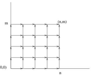
m (n,m)

Figure 2.1: All possible paths from (0,0) to (n, m)

Coolen [12] derived these NPI lower and upper probabilities through direct count-ing arguments. The method uses the appropriateA(n) assumptions [35] for inference

onm future random quantities givenn observations, and a latent variable represen-tation with Bernoulli quantities represented by observations on the real line, with a threshold such that successes are to one side and failures to the other side of the threshold. Under these assumptions, the (n+_nm) different orderings of these obser-vations, when not distinguishing between then observed values nor between the m future observations, are all equally likely. For each such an ordering, the success-failure threshold can be in any of then+m+ 1 intervals of the partition of the real line created by then+m values of the latent variables, leading ton+m+ 1 possible combinations (s, r), with s successes in the n tests and r successes in the m future observations.

For such an ordering, these possible (s, r) can be represented as a path on the rectangular lattice from (0,0) to (n, m) with steps going either one to the right or one upwards (see Figure 2.1). The (n+_nm) different orderings, which are all equally likely, correspond to the (n+_nm) different right-upwards paths from (0,0) to (n, m), and hence the above NPI lower and upper probabilities can also be derived by counting paths. To derive the NPI lower probability P(Y_nn₊₁+m ∈ Rt|Y1n = s),

2.2. NPI for Bernoulli quantities 13

k

(0,0) s−1 s n

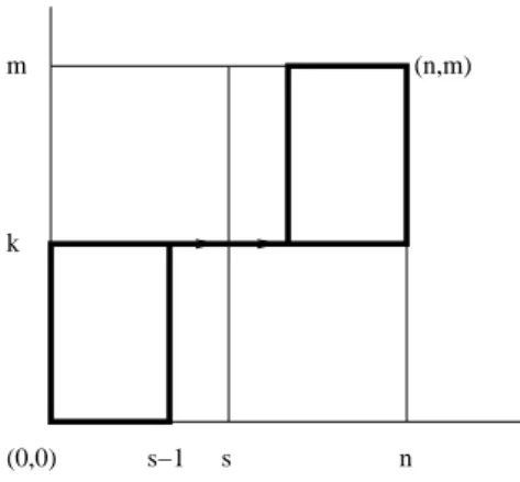
m (n,m)

Figure 2.2: all paths from (0,0) to (n, m) that pass through (s−1, k) and (s+ 1, k)

s n

(n,m)

(0,0) k

m

Figure 2.3: All paths from (0,0) to (n, m) via (s, k)

r ∈ Rt, so they do not go through (s, l) for any l ∈ Rct. The corresponding NPI

upper probability P(Y_nn₊₁+m ∈Rt|Y1n =s) is derived by counting all such paths that

go through at least one (s, r) with r ∈Rt. For example, the NPI lower probability

for the event (Y_nn₊₁+m =k |Yn

1 =s) can be derived by counting the paths from (0,0)

to (n, m) that pass through the two points (s−1, k) and (s+ 1, k) respectively (see Figure 2.2). The number of these paths is(s−_s−1+₁k)(n−s−_m1+_−km−k), hence

P(Y_nn₊₁+m =k|Y₁n =s) = ( n+m n )₋1[( s−1 +k s−1 )( n−s−1 +m−k m−k )]

The corresponding NPI upper probability can be derived by counting all paths from (0,0) to (n, m) via (s, k) (see Figure 2.3). The number of these paths is

(_s+k s )(_n−s+m−k n−s ) , hence P(Y_nn₊₁+m =k |Y₁n =s) = ( n+m n )₋1[( s+k s )( n−s+m−k n−s )]

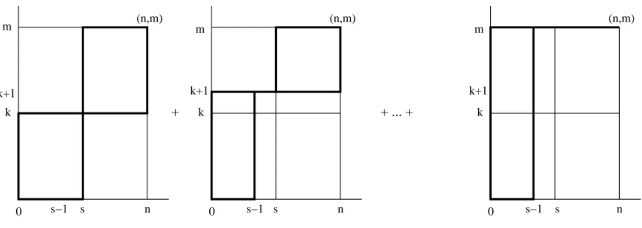
2.3. NPI for a k-out-of-m system 14 + + ... + 0 0 0 (n,m) (n,m) (n,m) k k k k+1 k+1 k+1 s s−1 s s−1 s s−1 m n m n n m

Figure 2.4: All paths which are counted in the upper probability (2.1)

In the next section, these results of NPI for Bernoulli data, are used to compute upper and lower probabilities for successful functioning ofk-out-of-m systems.

2.3

NPI for a

k

-out-of-

m

system

When considering a k-out-of-m system, the event Y_nn₊₁+m ≥ k is of interest as this corresponds to successful functioning of a k-out-of-m system, following n tests of components that are exchangeable with themcomponents in the system considered. Given data consisting of s successes from n components tested, the NPI lower and upper probabilities for the event that the k-out-of-m system functions successfully are also denoted by P(S(m : k)|(n, s)) and P(S(m :k)|(n, s)), respectively. From the NPI upper probability for Y_nn₊₁+m ∈ Rt given above, P(S(m : k)|(n, s)) follows

easily. For k∈ {1,2, . . . , m}and 0< s < n, P(S(m:k)|(n, s)) =P(Y_nn₊₁+m ≥k|Y₁n =s) = ( n+m n )−1 × [( s+k s )( n−s+m−k n−s ) + m ∑ l=k+1 ( s+l−1 s−1 )( n−s+m−l n−s )] (2.1)

This NPI upper probability can also be derived by counting all such paths that go through at least one point (s, r) with r≥k. To avoid that no path is counted more than once, the number of these paths can be computed by counting all paths from (0,0) to (n, m) via (s, k), in addition to paths from (0,0) to (n, m) via at least one of (s−1, k+ 1),(s−1, k+ 2),(s−1, k+ 3), . . . ,(s−1, m) (see Figure 2.4). The

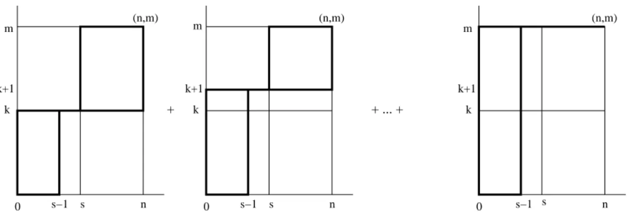
2.3. NPI for a k-out-of-m system 15 + + ... + 0 s−1 s 0 s−1 s 0 s−1 s k k k k+1 k+1 k+1 (n,m) (n,m) (n,m) n m m n m n

Figure 2.5: All paths which are counted in the lower probability (2.2)

corresponding NPI lower probability can be derived via the conjugacy property or by counting all paths which go through (s, r) forr≥k but not through any point (s, r) withr less thank. The number of these paths is equal to the number of paths from (0,0) to (n, m) via at least one of (s−1, k),(s−1, k+ 1),(s−1, k+ 2), . . . ,(s−1, m) (see Figure 2.5). P(S(m:k)|(n, s)) =P(Y_nn₊₁+m ≥k|Y₁n=s) = 1−P(Y_nn₊₁+m ≤k−1|Y₁n=s) = 1− ( n+m n )₋1[_∑k−1 l=0 ( s+l−1 s−1 )( n−s+m−l n−s )] (2.2)

Form= 1, so considering a system consisting of just a single component, the NPI upper and lower probabilities for the event that the system functions successfully are

P(S(1 : 1)|(n, s)) =P(Y_nn₊₁+1= 1|Y₁n=s) = s+ 1

n+ 1

P(S(1 : 1)|(n, s)) =P(Y_nn₊₁+1= 1|Y₁n=s) = s

n+ 1

If the observed data are all successes, so s = n, or all failures, so s = 0, then the NPI upper probabilities are, for allk ∈ {1, . . . , m},

P(S(m:k)|(n, n)) =P(Y_nn₊₁+m ≥k|Y₁n=n) = 1 P(S(m:k)|(n,0)) =P(Y_nn₊₁+m≥k|Y₁n= 0) = ( n+m−k n )( n+m n )₋1

and the NPI lower probabilities are, for all k ∈ {1, . . . , m},

P(S(m:k)|(n, n)) =P(Y_nn₊₁+m≥k|Y₁n=n) = 1− ( n+k−1 n )( n+m n )₋1 P(S(m:k)|(n,0)) =P(Y_nn₊₁+m ≥k|Y₁n= 0) = 0

2.3. NPI for a k-out-of-m system 16 n (0,0) k s s+1 m (n,m)

Figure 2.6: All paths which are counted in (2.3)

One of the results that actually holds generally for the NPI lower and upper probabilities for allk-out-of-m systems as considered in this thesis is

P(S(m:k)|(n, s)) =P(S(m :k)|(n, s+ 1)) (2.3) A direct proof of (2.3) can be easily achieved by using a path counting technique. Figure 2.6 shows that the paths that go through at least one point (s, r) withr ≥k (which are counted in the NPI upper probability for successful system functioning givenssuccesses inntests) ara exactly the same paths that go through (s+ 1, r) for r≥k but not through any point (s+ 1, r) with r less than k (which are counted in the NPI lower probability for successful system functioning given s+ 1 successes).

2.3.1

Examples of

k

-out-of-

m

systems

In this subsection two examples are presented to illustrate NPI for reliability of k-out-of-m systems, and some related issues are discussed.

Example 2.1

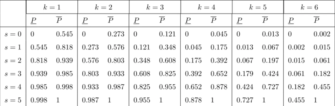
Consider a k-out-of-6 system. Table 2.1 provides the NPI lower and upper proba-bilities for all possible cases with n = 5 components tested, of which s functioned successfully, and withk varying from 1 to 6. The values in Table 2.1 illustrate some of the general properties for allk-out-of-m systems. The NPI upper probability for successful system functioning givens successes in n tests is equal to the NPI lower

2.3. NPI for a k-out-of-m system 17 k= 1 k= 2 k= 3 k= 4 k= 5 k= 6 P P P P P P P P P P P P s= 0 0 0.545 0 0.273 0 0.121 0 0.045 0 0.013 0 0.002 s= 1 0.545 0.818 0.273 0.576 0.121 0.348 0.045 0.175 0.013 0.067 0.002 0.015 s= 2 0.818 0.939 0.576 0.803 0.348 0.608 0.175 0.392 0.067 0.197 0.015 0.061 s= 3 0.939 0.985 0.803 0.933 0.608 0.825 0.392 0.652 0.179 0.424 0.061 0.182 s= 4 0.985 0.998 0.933 0.987 0.825 0.955 0.652 0.878 0.424 0.727 0.182 0.455 s= 5 0.998 1 0.987 1 0.955 1 0.878 1 0.727 1 0.455 1

Table 2.1: NPI lower and upper probabilities for all possible cases withn = 5

probability for successful system functioning given s+ 1 successes. The value 0 (1) of the NPI lower (upper) probability for the cases = 0 (s = 5) reflects that in this case there is no strong evidence that the components can actually function (fail). In order to get a reasonably large NPI lower probability for successful system func-tioning, it is not necessarily required that most tested components functioned well if k is small, which means that the system has much built-in redundancy, but for large values of k (nearly) all tested components must have been successful. Table 2.1 shows that the lower and upper probabilities are decreasing ink when keeping m, n and s constant, and increasing in s when keeping m, n and k constant. This is most obvious from the large differences between the values at the top left and bottom right of Table 2.1.

Example 2.2

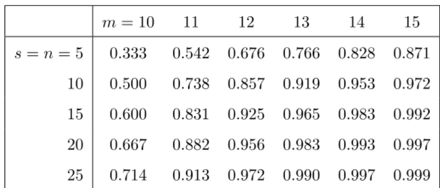
Consider a 10-out-of-m system. Suppose that, to increase the system’s reliability by increasing redundancy, extra components can be added to the system, keeping k= 10 but increasing the value of m. Assuming zero-failure testing, the NPI lower probabilities for the event that this system functions successfully are presented in Table 2.2 , for n = 5,10,15,20,25, and m varying from 10 to 15. Of course, the corresponding NPI upper probabilities are all equal to one as there are no failed components. Table 2.2 shows that the system’s reliability as measured by NPI lower probability is increasing inm, keeping n and k constant, and increasing in n, keepingm and k constant.

2.4. Series of independent ki-out-of-mi subsystems 18 m= 10 11 12 13 14 15 s=n= 5 0.333 0.542 0.676 0.766 0.828 0.871 10 0.500 0.738 0.857 0.919 0.953 0.972 15 0.600 0.831 0.925 0.965 0.983 0.992 20 0.667 0.882 0.956 0.983 0.993 0.997 25 0.714 0.913 0.972 0.990 0.997 0.999 Table 2.2: NPI lower probabilities for the systems in Example 2.2

The NPI lower probabilities presented in Table 2.2 can be used in several ways. For example, consider the case m = 10 with 5 zero-failure tests, leading to NPI lower probability 0.333 for successful system functioning. The table shows that increasing the redundancy tom = 11, keepingk = 10, would increase the NPI lower probability to 0.542, while increasing the number of zero-failure tests to 10 would increase the NPI lower probability to 0.5, so if these two actions were available at similar costs, increase of redundancy might be preferred to more tests. However, if 15 tests were possible at a cost similar to the cost of adding one component to the system, then this might be preferred, as the corresponding NPI lower probability would increase to 0.6 if all 15 tests were successes. Of course, we do not know if extra tested components would all function successfully.

Table 2.3 extends this example by presenting the minimum number of zero-failure tests required to achieve a chosen value for the NPI lower probability for successful system functioning, again fork = 10 andmvarying from 10 to 15. The requirement considered isP(S(m : 10)|(n, n))≥p for different values ofp.

The main conclusion from Table 2.3 is that the system’s reliability, as measured by NPI lower probability, can be increased either by having more successful tests or by building in redundancy.

2.4

Series of independent

k

-out-of-

m

subsystems

Coolen-Schrijner et al. [29] used the results for a k-out-of-m system straightfor-wardly to consider the reliability of systems that consist of a series configuration

2.4. Series of independent ki-out-of-mi subsystems 19 m= 10 11 12 13 14 15 p= 0.75 30 11 7 5 4 4 0.80 40 13 8 6 5 4 0.85 57 17 10 7 6 5 0.90 90 23 13 9 7 6 0.95 190 37 19 13 10 8 0.99 990 95 40 25 18 15

Table 2.3: Values of n required to achieve chosen values ofp.

of L ≥ 2 independent subsystems, with subsystem i (i = 1, . . . , L) a ki-out-of-mi system consisting of exchangeable components. As before, it is assumed that, in relation to subsystemi,ni components that are exchangeable with those to be used in the subsystem have been tested, of which si _{functioned successfully. For the}

se-ries system to function, all its subsystems must function, and due to the assumed independence of the subsystems (which implies independence of components in dif-ferent subsystems), the NPI lower and upper probabilities for such a series system to function are P(S[L](m1 :k1, . . . , mL:kL)|(n, s)) = L ∏ i=1 P(S(mi :ki)|(ni, si)) (2.4) and P(S[L](m1 :k1, . . . , mL:kL)|(n, s)) = L ∏ i=1 P(S(mi :ki)|(ni, si)) (2.5) Coolen-Schrijner et al. [29] considered optimal redundancy allocation for such systems, that is how best to assign additional components to subsystems (hence to increase the number of componentsmi), for situations where the required number of components that must function for the subsystems remains the same (ki_{). However,}

they only considered such redundancy allocation after zero-failure testing (sosi =ni for all i = 1, . . . , L), for which case they derived a powerful algorithm for optimal redundancy allocation, with the lower probability for system functioning used as the reliability measure. The NPI lower and upper probabilities for such a series system to function are illustrated and discussed in the following example.

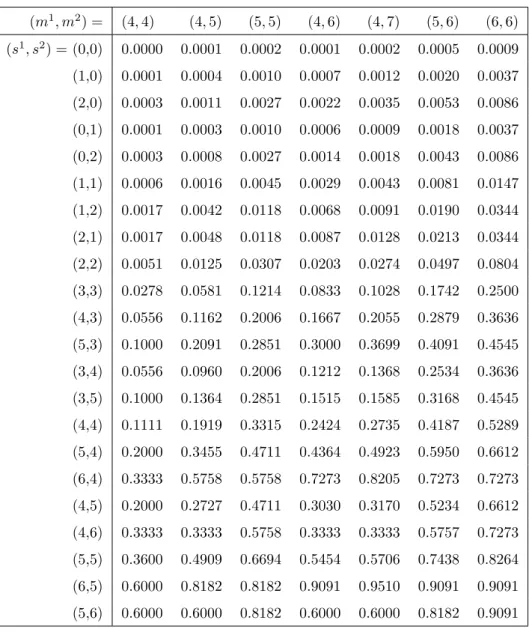
2.4. Series of independent ki-out-of-mi subsystems 20 (m1, m2) = (4,4) (4,5) (5,5) (4,6) (4,7) (5,6) (6,6) (s1, s2) = (1,1) 0.0000 0.0001 0.0002 0.0001 0.0002 0.0005 0.0009 (1,2) 0.0001 0.0003 0.0010 0.0006 0.0009 0.0018 0.0037 (2,1) 0.0001 0.0004 0.0010 0.0007 0.0012 0.0020 0.0037 (2,2) 0.0006 0.0016 0.0045 0.0029 0.0043 0.0081 0.0147 (3,3) 0.0051 0.0125 0.0307 0.0203 0.0274 0.0497 0.0804 (4,3) 0.0119 0.0292 0.0611 0.0473 0.0639 0.0988 0.1418 (5,3) 0.0238 0.0584 0.1009 0.0945 0.1278 0.1633 0.2062 (3,4) 0.0119 0.0249 0.0611 0.0357 0.0440 0.0877 0.1418 (3,5) 0.0238 0.0411 0.1009 0.0519 0.0586 0.1275 0.2062 (4,4) 0.0278 0.0581 0.1214 0.0833 0.1028 0.1742 0.2500 (5,4) 0.0556 0.1162 0.2006 0.1667 0.2055 0.2879 0.3636 (6,4) 0.1000 0.2091 0.2851 0.3000 0.3699 0.4091 0.4545 (4,5) 0.0556 0.0960 0.2006 0.1212 0.1368 0.2534 0.3636 (4,6) 0.1000 0.1364 0.2851 0.1515 0.1585 0.3168 0.4545 (5,5) 0.1111 0.1919 0.3315 0.2424 0.2735 0.4187 0.5289 (6,5) 0.2000 0.3455 0.4711 0.4364 0.4923 0.5950 0.6612 (5,6) 0.2000 0.2727 0.4711 0.3030 0.3170 0.5234 0.6612 (6,6) 0.3600 0.4909 0.6694 0.5454 0.5706 0.7438 0.8264 Table 2.4: NPI lower probability for system functioning

Example 2.3

Consider a system which consists of two independent subsystems (so L = 2) in a series configuration, where for each subsystem 4 exchangeable components must function to ensure that the subsystem functions, hence k1 _{= k}2 _{= 4, and where 6}

components exchangeable with those in subsystem 1 have been tested, and also 6 components exchangeable with those in subsystem 2 have been tested, son1 _=n2 ₌

6. Tables 2.4 and 2.5 present the NPI lower and upper probabilities, respectively, for functioning of this system, for varying numbers of test successes (s1 _ands2_{) and}

different numbers of components (m1 and m2) in these ki-out-of-mi subsystems. Test results for which the NPI lower probability for system functioning is zero (s1 = 0 or s2 = 0) are deleted from Table 2.4, the case s1 =s2 = 6 is deleted from

2.4. Series of independent ki-out-of-mi subsystems 21 (m1_{, m}2_{) = (4,4) (4,5) (5,5) (4,6) (4,7) (5,6) (6,6)} (s1_{, s}2_{) = (0,0) 0.0000 0.0001 0.0002 0.0001 0.0002 0.0005 0.0009} (1,0) 0.0001 0.0004 0.0010 0.0007 0.0012 0.0020 0.0037 (2,0) 0.0003 0.0011 0.0027 0.0022 0.0035 0.0053 0.0086 (0,1) 0.0001 0.0003 0.0010 0.0006 0.0009 0.0018 0.0037 (0,2) 0.0003 0.0008 0.0027 0.0014 0.0018 0.0043 0.0086 (1,1) 0.0006 0.0016 0.0045 0.0029 0.0043 0.0081 0.0147 (1,2) 0.0017 0.0042 0.0118 0.0068 0.0091 0.0190 0.0344 (2,1) 0.0017 0.0048 0.0118 0.0087 0.0128 0.0213 0.0344 (2,2) 0.0051 0.0125 0.0307 0.0203 0.0274 0.0497 0.0804 (3,3) 0.0278 0.0581 0.1214 0.0833 0.1028 0.1742 0.2500 (4,3) 0.0556 0.1162 0.2006 0.1667 0.2055 0.2879 0.3636 (5,3) 0.1000 0.2091 0.2851 0.3000 0.3699 0.4091 0.4545 (3,4) 0.0556 0.0960 0.2006 0.1212 0.1368 0.2534 0.3636 (3,5) 0.1000 0.1364 0.2851 0.1515 0.1585 0.3168 0.4545 (4,4) 0.1111 0.1919 0.3315 0.2424 0.2735 0.4187 0.5289 (5,4) 0.2000 0.3455 0.4711 0.4364 0.4923 0.5950 0.6612 (6,4) 0.3333 0.5758 0.5758 0.7273 0.8205 0.7273 0.7273 (4,5) 0.2000 0.2727 0.4711 0.3030 0.3170 0.5234 0.6612 (4,6) 0.3333 0.3333 0.5758 0.3333 0.3333 0.5757 0.7273 (5,5) 0.3600 0.4909 0.6694 0.5454 0.5706 0.7438 0.8264 (6,5) 0.6000 0.8182 0.8182 0.9091 0.9510 0.9091 0.9091 (5,6) 0.6000 0.6000 0.8182 0.6000 0.6000 0.8182 0.9091

Table 2.5: NPI upper probability for system functioning

Table 2.5 as the corresponding NPI upper probability is one for allm1 _{and m}2_.

These tables illustrate the manner in which system reliability, measured by these NPI lower and upper probabilities, increases with increasing numbers of test suc-cesses and with increasing system redundancy. They also illustrate that, as the propertyP(S(m:k)|(n, s)) =P(S(m:k)|(n, s+ 1)) still holds per subsystem, for the whole system P(S[L](m1 : k1, . . . , mL : kL) | (n, s)) = P(S[L](m1 : k1, . . . , mL : kL₎|_{(n, s+ 1)), where the elements of s+ 1 is obtained by adding one to each}

ele-ment ofs. For example, the NPI upper probabilities for (s1, s2) equal to (1,1), (2,2), (3,3), (3,4), (4,3) and (4,4) are equal to the corresponding NPI lower probabilities

2.5. Redundancy allocation 22

for (s1, s2) equal to (2,2), (3,3), (4,4), (4,5), (5,4) and (5,5) respectively. Note that in situations where for a particular subsystem all performed tests are successes, the NPI upper probability for system functioning is in fact the NPI upper probability that the other subsystem functions. For example, in Table 2.5 for (s1_{, s}2_{) = (6,5), the}

NPI upper probabilities for system functioning with (m1_{, m}2_{) equal to (4,6),(5,6)}

and (6,6) are identical and equal to the NPI upper probability that subsystem 2, a 4-out-of-6 subsystem, functions.

The next section introduces a generalization of the optimal redundancy allocation algorithm by Coolen-Schrijner et al. [29] to general test results. It is particularly logical to focus attention on the NPI lower probability in this generalization, as the lower probability can be considered to be a conservative inference.

2.5

Redundancy allocation

The systems considered in this section consist of series configurations of L inde-pendent ki_-out-of-mi _{subsystems, and information about reliability of components}

results from tests in which, for subsystem i, ni _{components that are exchangeable}

with those in subsystemihave been tested, of whichsi _{functioned successfully. From}

now on, it is assumed that si _{≥ 1 for all i = 1, . . . , L, in order to avoid problems}

occurring due to the fact that the NPI lower probability for successful functioning of a ki_-out-of-mi _{system is equal to zero if s}i _{= 0, for all n}i_{, k}i_{, m}i_{. In practice, it}

is unlikely that one would wish to proceed with components of which none func-tioned successfully in testing, so this assumption seems not to limit the practical applicability of the method proposed here in a significant manner.

2.5.1

Redundancy allocation algorithm

With reliability measured by the NPI lower probability for system functioning, op-timal redundancy allocation of extra components can be achieved (as we prove in the next section), for any number of extra components, by sequential one-step op-timal allocation. According to this technique, at each step an extra component is allocated to the subsystem for which the relative increase in reliability is maximal.

2.5. Redundancy allocation 23

The algorithm to determine the optimal sequence of adding the extra components to subsystems is described below, where optimality is in the sense of maximum NPI lower probability.

The NPI lower probability for successful functioning of the whole system, fol-lowing ni _{tests of components exchangeable with those in subsystem i of which s}i

functioned successfully, is P(S[L]_(m1 _{: k}1_{, . . . , m}L _{: k}L_{) | (n, s)) as given by (2.4).}

Now consider the situation withji _{additional components added to subsystemi, for}

i = 1, . . . , L, with no further tests performed, then the NPI lower probability for successful functioning of the system becomes

P(S[L](m1+j1 :k1, . . . , mL+jL :kL)|(n, s)) =

L

∏

i=1

P(S(mi+ji :ki)|(ni, si)) Optimal allocation of (any number of) additional components, to enhance the system reliability, can be achieved by adding the components in an optimal sequence ac-cording to the following algorithm (given in pseudo-code), in which, fori= 1, . . . , L and ji _≥0,

ρ(i, ji) = P(S(m

i_+ji_{+ 1 :k}i_)|(ni_{, s}i₎₎

P(S(mi_+ji _:ki₎|_(ni_{, s}i₎₎

Soρ(i, ji) is the factor by which the NPI lower probability for successful functioning of subsystem i increases when ji _{+ 1 instead of j}i _{extra components are added}

to subsystem i, hence this represents the relative increase in reliability of both subsystemi and the whole system.

Optimal allocation algorithm

1. Set ji = 0 and calculate ρ(i, ji) =ρ(i,0) for all i= 1, . . . , L;

2. Determine im such that

ρ(im, jim) = max

1≤i≤Lρ(i, j i₎

If this im is not a unique value, then, according to one-step-at-a-time

opti-misation, pick any one of these values (from the proof of optimality of this algorithm, as presented in Subsection 2.5.2, it follows that in case of multiple

2.5. Redundancy allocation 24

maxima these can be taken in any order without affecting the optimal lower probability of system functioning at any stage);

3. Add an extra component to subsystem im: set jim := jim + 1 and calculate

ρ(im, jim);

4. Return to Step 2, using the same values ρ(i, ji) as in the previous step fori6= im, together with the new valueρ(im, jim) for subsystemim, as just calculated

in Steps 2 and 3.

This algorithm can be stopped at any time, whatever stop-criterion is defined, and will always give optimal allocation of extra components. After stopping the algorithm, the vector j = (j1_{, . . . , j}L_{) gives the number of extra components added}

to each subsystem, and the NPI lower probability for successful functioning of the system after adding these extra components is equal to

P(S[L](m1+j1 :k1, . . . , mL+jL :kL)|(n, s)) = P(S[L](m1 :k1, . . . , mL :kL)|(n, s))× L ∏ i=1 ji₋₁ ∏ li₌₀ ρ(i, li).

This enables easy calculation of the NPI lower probability following Step 3 of the above algorithm, as it just requires the previous value of this NPI lower probability to be multiplied by theρ(im, jim) calculated at that step.

2.5.2

Optimality of redundancy allocation algorithm

It is claimed that the sequential one-step redundancy allocation algorithm presented in Section 2.5.1 provides overall optimality in the sense of maximum NPI lower prob-ability for successful functioning of the system, no matter how many components can be added in total, or indeed how the number of extra components is deter-mined. The proof of this optimality is given below with some change of notation for convenience.

Let ν(n, m) denote the number of equally likely orderings of those variables for which the dataYn

2.5. Redundancy allocation 25 Letλ(n, m) =P(m:k |n, s), so λ(n, m) = ( n+m n )−1 ν(n, m) (2.6)

For (n, m) such that n+m≥s+k these λ(n, m) are λ(n, m) =          P(Y_nn₊₁+m ≥k |Y₁n =s), n ≥s, m≥k 1, 0< n≤s−1, 0, 0< m≤k−1 .

As ν counts paths the following key equation holds

ν(n, m+ 1) =ν(n, m) +ν(n−1, m+ 1), n+m≥s+k and by employing standard binomial identities

(n+m+ 1)λ(n, m+ 1) = (m+ 1)λ(n, m) +nλ(n−1, m+ 1) . (2.7) Whens = 1 andk = 1 the simple formλ(n, m) = m/(n+m) holds forn+m≥1.

It was shown by Coolen-Schrijner et al. [29] that {λ(s, m)}m is increasing and

log-concave, specifically{λ(s, m) :m ≥k}is increasing inm,{λ(s, m+1)/λ(s, m)) : m ≥ k} is decreasing in m. To prove that the redundancy allocation algorithm in the previous section is optimal, these results need to be generalized to the case of general n. The first step is establishing monotonicity for each n, working with diagonal sets of nodes, i.e. with n+m fixed.

Lemma 2.1. For any n ≥s, t≥s+k,

1. {λ(t−m, m) :k−1≤m ≤t} is increasing in m; 2. {λ(n, m) :m≥k−1} is increasing in m.

Proof.

1. This is true fort =s+k as 0< s/(s+k)<1. Suppose it is true fort ≥s+k and consider the sequence for t+ 1. By (2.7)

λ(t−m, m+ 1) = m+ 1 t+ 1 λ(t−m, m) + t−m t+ 1 λ(t−m−1, m+ 1) > λ(t−m, m) (induc. hyp.) (2.8) > m t+ 1 λ(t+ 1−m, m−1) + t+ 1−m t+ 1 λ(t−m, m) =λ(t+ 1−m, m) (by (2.7) )

2.5. Redundancy allocation 26

and the result holds for all t≥s+k by induction.

2. By (2.8), for any n≥s,λ(n, m+ 1)> λ(n, m) form≥k.

Now the ratiosλ(n, m+ 1)/λ(n, m) are considered. It is slightly more convenient to work with the reciprocalsλ(n, m)/λ(n, m+ 1). Once again working with diagonal sets of nodes proves to be easiest.

Lemma 2.2. For each t=s+k+ 1, s+k+ 2, . . . the sequence of ratios

{λ(t−m, m−1)/λ(t+ 1−m, m) :k≤m ≤t+ 1−s} is increasing in m.

Proof. The caset =s+k+ 1 is readily established by direct calculation. Suppose that the result has been established for some t−1 where t ≥s+k+ 2. Introduce the notation `m = λ(t−1−m, m), Lm =λ(t−m, m) to simplify the expressions.

Next it is shown that{Lm−1/Lm :m≥k} is increasing. Using (2.7)

Lm Lm+1 = m`m−1+ (t−m)`m (m+ 1)`m+ (t−1−m)`m+1 , Lm−1 Lm = (m−1)`m−2+ (t+ 1−m)`m−1 m`m−1 + (t−m)`m

so (after cross-multiplying) the aim is to show that

L2_m−Lm+1Lm−1 >0 for m =k, k+ 1, . . . , t+ 1−s . (2.9)

From the induction hypothesis it follows that ∆2

m ≡ `2m−`m+1`m−1 > 0 for m =

k,. . ., t−s and similarly that for k+ 1 ≤m≤t+ 1−s, Γ1 ≡`m`m−1−`m+1`m−2 =`m+1`m−1 ( `m `m+1 − `m−2 `m−1 ) >0 (Γ1 = 0 when m=k since `k−1 =`k−2 = 0). Further from Lemma 2.1

Γ2 ≡`m`m−2+`m+1`m−1−`m+1`m−2−`m`m+1 = (`m−2−`m−1)(`m−`m+1)>0

fork+1≤m≤t−swith Γ2 = 0 whenm=korm=t+1−s. Fork ≤m≤t+1−s

t2(L2_m−Lm+1Lm−1) =m2∆2m−1+ (t−m)

2_∆2

m+

(

m(t−m)−t)Γ1+ Γ2 >0

as m(t−m) > t. Thus (2.9) holds and the result for all t ≥ s+k + 1 follows by induction.

2.5. Redundancy allocation 27 Theorem 2.1. For any fixed n≥s,

λ(n, m) λ(n, m+ 1) >

λ(n, m−1)

λ(n, m) for m≥k.

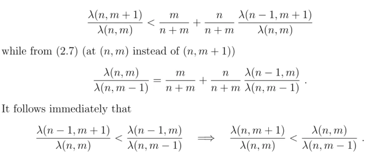
Proof. The inequality is trivial whenm =k so supposem ≥k+ 1. From (2.7) and Lemma 2.1 (1) λ(n, m+ 1) λ(n, m) < m n+m + n n+m λ(n−1, m+ 1) λ(n, m) while from (2.7) (at (n, m) instead of (n, m+ 1))

λ(n, m) λ(n, m−1) = m n+m + n n+m λ(n−1, m) λ(n, m−1) . It follows immediately that

λ(n−1, m+ 1) λ(n, m) < λ(n−1, m) λ(n, m−1) =⇒ λ(n, m+ 1) λ(n, m) < λ(n, m) λ(n, m−1) .

It is thus sufficient to show, in the notation of Lemma 2, thatLm+1/Lm < `m/`m−1.

ExpandingLm+1 and Lm using (2.7) and cross-multiplying leads to

[(m+ 1)`m+ (n−1)`m+1]`m−1 <[m`m−1 +n`m]`m

⇔ `m`m−1−`m+1`m−1 < n(`2m−`m+1`m−1)

⇔ `m−1(`m−`m+1)< n∆2m .

By Lemma 2.1 (1) the left-hand term is negative and by Lemma 2.2 the right-hand term is positive so the result is established.

Example 2.4

The redundancy allocation algorithm presented in Section 2.5.1 is illustrated via a basic system consisting initially of four independent ki_-out-of-mi _{subsystems in}

series configuration with the valueski_andmi _{as given in Table 2.6. Several scenarios}

of allocation of additional components, to increase redundancy optimally, will be illustrated for this system, with different numbers of successes in the tests of different components. Throughout this example, we assume that 5 components of each type were tested, soni _{= 5 for i= 1, . . . ,4.}

Table 2.7 presents the optimal allocation sequences of 5 extra components for zero-failure tests and for tests in which a single component of one type failed. In

2.5. Redundancy allocation 28 i ki mi 1 1 2 2 2 3 3 3 5 4 1 4

Table 2.6: Subsystemi: ki_-out-of-mi

(s1, s2, s3, s4) sequence initial reliability final reliability (5,5,5,5) 2-3-1-2-3 0.7733 0.9259 (4,5,5,5) 1-2-3-1-2 0.6960 0.8877 (5,4,5,5) 2-2-3-2-1 0.6186 0.8677 (5,5,4,5) 3-2-3-3-1 0.6227 0.8479 (5,5,5,4) 2-3-1-2-3 0.7485 0.8963 Table 2.7: Optimal allocation sequences of 5 components

addition, for each case, the initial reliability of the system is given, so before any extra components have been allocated, as well as the final reliability after the 5 extra components have been allocated according to the optimal sequence.

For example, in the second case in Table 2.7, where one component exchangeable with those in subsystem 1 (say ‘of type 1’) has failed during testing, the optimal allocation of 5 extra components, to achieve maximal improvement of reliability of the overall system, is to first assign an extra component to subsystem 1, then one to subsystem 2, followed by extra components to subsystems 3, 1 and 2, in that order. It is clear from this example, and also obvious from the optimal allocation algorithm presented above, that if a tested component of a specific type has failed, then the corresponding subsystem tends to be assigned one or more extra components earlier in the optimal sequence when compared to the same system but without that test failure. If this happens, the order of added components for the other subsystems, for which no corresponding tested components failed during testing, remains unchanged.