Latin hypercube sampling with dependence and applications in finance

econ

stor

www.econstor.eu

Der Open-Access-Publikationsserver der ZBW – Leibniz-Informationszentrum Wirtschaft

The Open Access Publication Server of the ZBW – Leibniz Information Centre for Economics

Nutzungsbedingungen:

Die ZBW räumt Ihnen als Nutzerin/Nutzer das unentgeltliche, räumlich unbeschränkte und zeitlich auf die Dauer des Schutzrechts beschränkte einfache Recht ein, das ausgewählte Werk im Rahmen der unter

→ http://www.econstor.eu/dspace/Nutzungsbedingungen nachzulesenden vollständigen Nutzungsbedingungen zu vervielfältigen, mit denen die Nutzerin/der Nutzer sich durch die erste Nutzung einverstanden erklärt.

Terms of use:

The ZBW grants you, the user, the non-exclusive right to use the selected work free of charge, territorially unrestricted and within the time limit of the term of the property rights according to the terms specified at

→ http://www.econstor.eu/dspace/Nutzungsbedingungen By the first use of the selected work the user agrees and declares to comply with these terms of use.

zbw

Packham, Natalie; Schmidt, Wolfgang M.

Working Paper

Latin hypercube sampling with

dependence and applications in finance

Provided in cooperation with:

Frankfurt School of Finance and Management

Suggested citation: Packham, Natalie; Schmidt, Wolfgang M. (2008) : Latin hypercube sampling with dependence and applications in finance, CPQF Working Paper Series, No. 15, http:// hdl.handle.net/10419/40177

C

C

e

e

n

n

t

t

r

r

e

e

f

f

o

o

r

r

P

P

r

r

a

a

c

c

t

t

i

i

c

c

a

a

l

l

Q

Q

u

u

a

a

n

n

t

t

i

i

t

t

a

a

t

t

i

i

v

v

e

e

F

F

i

i

n

n

a

a

n

n

c

c

e

e

No. 15

Latin hypercube sampling with dependence

and applications in finance

Natalie Packham, Wolfgang Schmidt

October

2008

Authors: Prof. Dr. Wolfgang M. Schmidt Natalie Packham Frankfurt School of Frankfurt School of Finance & Management Finance & Management

Frankfurt/Main Frankfurt/Main

[email protected] [email protected]

Publisher: Frankfurt School of Finance & Management

Phone: +49 (0) 69 154 008-0 ƒ Fax: +49 (0) 69 154 008-728 Sonnemannstr. 9-11 ƒ D-60314 Frankfurt/M. ƒ Germany

Latin hypercube sampling with dependence and applications in finance

Natalie Packham and Wolfgang M. Schmidt

October 2008

Abstract:In Monte Carlo simulation, Latin hypercube sampling (LHS) [McKayet al.(1979)] is a well-known variance reduction technique for vectors of independent random variables. The method presented here, Latin hypercube sampling with dependence (LHSD), extends LHS to vectors of dependent random variables. The resulting estimator is shown to be consistent and asymptotically unbiased. For the bivariate case and under some conditions on the joint distribution, a central limit theorem together with a closed formula for the limit variance are derived. It is shown that for a class of estimators satisfying some monotonicity condition, the LHSD limit variance is never greater than the corresponding Monte Carlo limit variance. In some valuation examples of financial payoffs, when compared to standard Monte Carlo simulation, a variance reduction of factors up to 200 is achieved. LHSD is suited for problems with rare events and for high-dimensional problems, and it may be combined with Quasi-Monte Carlo methods.

Keywords: Monte Carlo simulation, variance reduction, Latin hypercube sampling, stratified sampling JEL classification: C15, C63, G12

Contents

1 Introduction . . . 2

2 Preliminaries . . . 4

3 Latin hypercube sampling with dependence . . . 5

4 Consistency of the LHSD estimator . . . 7

5 Central Limit Theorem for LHSD and variance reduction . . . 10

6 LHSD on random vectors with nonuniform marginals . . . 15

7 Applications in finance . . . 17

A Integration by parts formula . . . 22

1. Introduction

Consider the problem of reducing the variance of a Monte Carlo estimator targeted at a vector of dependent random variables. Many existing variance reduction techniques are powerful, but exploit particular properties of the problem at hand; see [Glasserman (2004), Section 4.7] for a comparison of variance reduction techniques taking into account their complexity and effectiveness. The method proposed here, Latin hypercube sampling with dependence (LHSD), is generally applicable, it is particularly simple, and it achieves an effective variance reduction for many estimation problems, including problems with rare events and high-dimensional problems. It is often effective even for low sample sizes, and it may easily be combined with other variance reduction techniques.

LHSD is a generalisation of a multivariate variance reduction technique known asLatin hyper-cube sampling (LHS), introduced by [McKay et al. (1979)] and further studied by [Stein (1987)] and [Owen (1992)], amongst others. LHS relies on independence of the components of the random vector involved. Essentially, LHSD extends LHS to random vectors with dependent components. The method is mentioned by [Stein (1987)], but, to the best of our knowledge, it has not been analysed in detail and no results about its effectiveness have been derived yet.

On a probability space (Ω,F,P), let (U1_{, . . . , U}d_{) be a random vector with uniform marginals}

and with copulaa _{C. Suppose the goal is to estimate}

Eg(U1, . . . , Ud) with g : [0,1]d → R

Borel-measurable andC-integrable.

The usual Monte Carlo estimator based onnindependent samples (U_i1, . . . , U_id),i= 1, . . . , n, is 1/nPn

i=1g(U 1

i, . . . , Uid). It is a strongly consistent estimator, i.e., 1/n

Pn i=1g(U 1 i, . . . , Uid) P–a.s. −→

Eg(U1, . . . Ud) as n → ∞. The central limit theorem for sums of independent random

vari-ables states that the scaled estimator converges in distribution to a Normal distribution, i.e., 1/√nPn i=1g(U 1 i, . . . , U d i) L

→ N(0, σ2), with σ2 = Var(g(U1, . . . , Ud)). The central limit theorem serves as an indicator of the speed of convergence via the approximation 1/nPn

i=1g(U 1

i, . . . , Uid)≈ X, for someX ∼N(0, σ2_{/n), from which we may derive confidence intervals and other statistics. In} general, the variance of an estimator is a key figure for assessing the quality of an estimation.

LHSD transformsnindependent samples (U1

i, . . . , Uid),i= 1, . . . , n, in such a way that for each

dimensionj, the marginalsU_ij,i= 1, . . . , n, are uniformly spread over [0,1]. At the same time, the transformation aims to preserve the copula. We show that the LHSD estimator of_Eg(U1_{, . . . , U}d_{) is}

strongly consistent for bounded and continuousg, and consistent for bounded andC-a.e. continuous

g. In the bivariate case, under some moderate conditions on the copulaCof the underlying random vector, we derive a central limit theorem, which states that the LHSD estimator converges to a Normal distribution. The central limit theorem is derived by applying a result from [Fermanian et al. (2004)]. We show that, under some monotonicity conditions on g, the limit variance of the LHSD estimator is never greater than the respective Monte Carlo limit variance.

Monte Carlo simulation is widely used for the valuation of financial claims. The general approach to value a financial claim is to generate sample paths of the underlying financial securities. The discounted expectation of the claim’s payoff under a risk-neutral measure is then an estimator of the claim’s fair value. For a comprehensive overview of Monte Carlo simulation in financial applications, we refer to [Glasserman (2004)].

We consider two examples of financial claims that depend on the joint distribution of several underlying assets. A first-to-default credit basket is valued based on random numbers and Sobol sequences, both with and without LHSD. The variance (resp. mean square error) of the LHSD estimators is between 2.25 and 4 times smaller compared to the corresponding estimators without LHSD. An interesting feature of the LHSD estimator is that, even though defaults are rare events, it guarantees that a fixed number of default events are sampled. The second example is concerned with the valuation of an Asian basket option, wich may be formulated as a high-dimensional estimation problem (dimension 2500 in the example). The variance reduction achieved depends on the strike of the option and lies between factors of 6 and 200.

The outline of the paper is as follows: In Section 2 we introduce stratified sampling, a univariate variance reduction technique, and its multivariate extension, Latin hypercube sampling. We present the LHSD method in Section 3. Section 4 contains statements about the consistency and unbiasedness of the LHSD estimator. In Section 5, restrictring ourselves to the bivariate case and under some conditions on the copula, we provide a central limit theorem and we analyse the rate of convergence of the LHSD estimator. In Section 6 we show that the LHSD estimator for random vectors with uniform marginals extends naturally to random vectors with nonuniform marginals. As example applications we consider the valuation of first-to-default credit baskets and Asian basket options in Section 7.

a_{A copulaCis the distribution function of a random vector with uniform marginals, see e.g. [Joe (1997)] and [Nelsen}

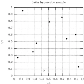
0 0.1 0.2 0.3 0.4 0.5 0.6 0.7 0.8 0.9 1.0 0.9 0.8 0.7 0.6 0.5 0.4 0.3 0.2 0.1 0 U 2 U1 Original sample 0 0.1 0.2 0.3 0.4 0.5 0.6 0.7 0.8 0.9 1 1.0 0.9 0.8 0.7 0.6 0.5 0.4 0.3 0.2 0.1 0 V 2 V1

Latin hypercube sample

Fig. 1. Left: Original sample (U1

1, U12), . . . ,(U101, U102), with (U11, U12) marked by a circle. Right: Corresponding Latin

hypercube sample, with (V1

1, V12) marked by a circle. The permutations areπ1={5,9,7,8,1,10,4,2,3,6}andπ2=

{1,7,9,6,3,2,5,10,4,8}.

2. Preliminaries

2.1. Stratified sampling

Stratified sampling is a variance reduction technique in a univariate setting that constrains the fraction of samples drawn from specific subsets, so-called strata. For a detailed exposition we refer to [Glasserman (2004), Chapter 4.3].

Suppose the goal is to estimate Eg(U) with U ∼ U(0,1) (i.e., a uniform random variable on

[0,1]), and with g : [0,1] → _R a Borel-measurable and integrable function. Let A1, . . . , An be a

partition of [0,1]. Then, Eg(U) = n X i=1 E(g(U)|U ∈Ai)P(U ∈Ai),

and a corresponding estimator of _Eg(U) is derived from sampling U conditional on {U ∈ Ai}, i = 1, . . . , n. In the simplest case, the strata are chosen to be the equiprobable intervals Ai =

((i−1)/n, i/n], i = 1, . . . , n, and one sample is drawn from each stratum. This is achieved for example by drawing independentU(0,1) samples,U1, . . . , Un, and setting

Vi:= i−1

n +

Ui

n, i= 1, . . . , n. (1)

The resulting estimator of _Eg(U), given by 1/nPn

i=1g(Vi), is consistent, and by a central limit theorem for the stratified estimator it follows that the limit variance is smaller than the Monte Carlo variance, cf. [Glasserman (2004), Section 4.3.1].

2.2. Latin hypercube sampling

Simply extending stratified sampling tod-dimensional random vectors by stratifying each dimension withnsamples is unfeasible even for moderately small dimensions, since to have one sample in each stratum requires at least nd _{samples. Latin hypercube sampling (LHS) efficiently extends stratified}

sampling to random vectors (U1, . . . , Ud) whose components are independent (i.e., they are linked by the independence copula). It was introduced in [McKayet al.(1979)] and further developed by [Stein (1987)] and [Owen (1992)]. For an in-depth treatment of LHS see [Glasserman (2004), Section 4.4].

Assume that the goal is to estimate Eg(U1, . . . , Ud) with g : [0,1]d → R Borel-measurable

and integrable. Fixing a sample size n, generaten independent samples (U1

and generatedindependent permutationsπ1_{, . . . , π}d _{of{1, . . . , n}drawn from the distribution that}

makes all permutations equally probable. Denoting byπ_ijthe value to whichiis mapped by thej-th permutation, a Latin hypercube sample is given by

V_ij:= π j i −1 n + U_ij n , j = 1, . . . , d, i= 1, . . . , n.

An example of a Latin hypercube sample is shown in Figure 1. Observe that in each dimension j, (V₁j, . . . , Vj

n) is a stratified sample. Furthermore, each point (Vi1, . . . , Vid), is uniformly distributed on

[0,1]d_{, 1≤i≤n. The LHS estimator 1/n}Pn

i=1g(Vi1, . . . , Vid) is consistent. [Stein (1987)] shows that,

for functions g with finite second moment, the variance of the LHS estimator is smaller compared to the standard Monte Carlo estimator as long as the number of samples is sufficiently large. For boundedg, [Owen (1992)] derives a central limit theorem for the LHS estimator.

Requiring independence of the components of the random vector is fundamental: Applying LHS to a sample of a random vector whose components are dependent destroys the dependence by application of random and independent permutations in each dimension. Conversely, applying first LHS to a sample of a random vector with independent components, and then applying a transform to introduce dependence breaks, in general, the stratification of the marginals, thereby losing much of the appeal of LHS.

3. Latin hypercube sampling with dependence

We now describe an extension of LHS for random vectors with dependence. The general idea is to generate a Latin hypercube sample, albeit with the following modification: Instead of choosing a random permutation in each dimension, a particular permutation that depends on the samples of that dimension is chosen. For this we need the notion of a rank statistic.

Definition 1 (Rank statistic). Let X1, . . . , Xn be i.i.d. random variables with continuous

dis-tribution function. Reorder them such that X(1) _{< . . . < X}(n) _{P–a.s.. The index of X}

i within X(1), . . . , X(n) is thei-th rank statistic, given by

ri,n(X1, . . . , Xn) := n

X

k=1

1_{Xk≤Xi}. (2)

That such an ordering existsP–a.s. follows from the continuity of the distribution function. For ease of notation, we write justri,ninstead ofri,n(X1, . . . , Xn).

Consider a random vector (U1_{, . . . , U}d_{), U}j _{∼ U(0,1), j = 1, . . . , d, whose components are}

linked by an arbitrary copula C, and let (U1

i, . . . , Uid), i = 1, . . . , n, ben independent samples of

(U1_{, . . . , U}d_{). For 1≤i≤nand 1≤j ≤ddenote byr}j

i,n thei-th rank statistic of (U j

1, . . . , Unj). A

Latin hypercube sample with dependence is given by

V_i,nj := r j i,n−1 n + ηj_i,n n , i= 1, . . . , n, j= 1, . . . , d, (3)

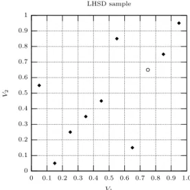
where η_i,nj are random variables taking values in [0,1], which we specify below. Figure 2 shows an example with 10 samples drawn from a bivariate Gaussian copula with correlation 1/2 and the corresponding LHSD samples.

Just as in regular LHS, (V₁j, . . . , Vj

n) is a stratified sample in each dimensionj. Recall that each

sample from the stratified sample of Equation (1) is uniformly distributed within its stratum. If

η_i,nj :=U_ij this property is lost by application of the rank statistic: in each dimension, the smallest sample is allocated to the first stratum, the second smallest to the second stratum, and so on. Conditional on {r_i,nj = k}, U_ij follows a beta distribution with parameters k and n, i.e., P(U_ij ≤ x|rj_i,n=k) =Bn

k(x), which is the distribution of thek-th order statistic of nindependent uniform

random variables, see e.g. [Feller (1971), Ch. I.7]. The following choices produce a LHSD sample with uniform marginals:

0 0.1 0.2 0.3 0.4 0.5 0.6 0.7 0.8 0.9 1 1.0 0.9 0.8 0.7 0.6 0.5 0.4 0.3 0.2 0.1 0 U2 U1 Original sample,ρ= 1/2 0 0.1 0.2 0.3 0.4 0.5 0.6 0.7 0.8 0.9 1 1.0 0.9 0.8 0.7 0.6 0.5 0.4 0.3 0.2 0.1 0 V2 V1 LHSD sample

Fig. 2. Left: Original sample (U1

1, U12), . . . ,(U101, U102) linked with a Gaussian copula with correlation ρ = 1/2;

(U1

1, U12) is marked by a circle. Right: Corresponding LHSD sample, with (V11,10, V12,10) marked by a circle. The rank

statistics arer1_{={8,6,1,4,3,7,5,2,9,10}andr}2_{={7,9,6,4,3,2,5,1,8,10}, andη}j

i,10:= 1/2,j= 1,2,i= 1, . . . ,10.

(i) η_i,nj :=Bn r_i,nj (U

j

i),i= 1, . . . , n, j= 1, . . . , d,

(ii) (η_i,nj )i=1,...,n;j=1,...,d is a sample of independent U(0,1) random variables independent of

(U_ij)i=1,...,n;j=1,...d.

If the primary goal is to capture the joint distribution, the following choices are computationally more efficient:

(iii) η_i,nj := 1/2, which places each sample in the middle of its stratum,

(iv) η_i,nj := 1, in which caseV_i,nj is just the empirical distribution function of (U₁j, . . . , Uj n) atU

j i, i= 1, . . . , n,j = 1, . . . , d.

Remark 2. LHS is a special case of LHSD: Let (U1_{, . . . , U}d_{) be independent, and let}

(ηj_i)i=1,...n;j=1,...d be chosen according to choice (ii). Then (U j

i)i=1,...,n;j=1,...,d determine

indepen-dent and equiprobable permutations that allocate samples to strata, and (η_ij)i=1,...n;j=1,...ddetermine

independently the position, uniformly distributed, of each sample in its stratum. Assume that the quantity to estimate is_Eg(U1_{, . . . , U}d_{) withg : [0,1]}d _→

R Borel-measurable

and integrable and (U1, . . . , Ud) a random vector with uniform marginals and copulaC. The LHSD estimator is given by 1 n n X k=1 g(V_i,n1 , . . . , V_i,nd ), (4)

with V_i,nj ,i= 1, . . . , n,j= 1, . . . , d, obtained from the transformation of Equation (3).

Before we analyse the estimator formally, let us reflect why it would reduce the variance: Vari-ance reduction over the usual Monte Carlo estimator is achieved by drawing “favourable” samples and avoiding “unfavourable” samples (i.e., samples with a large contribution to the variance of the estimator). For each dimension 1 ≤ j ≤d, LHSD ensures that the samples V₁j_,n, . . . , Vn,nj are

uniformly spread over the unit interval, thereby deleting inter-stratum variance and leaving only intra-stratum variance. As a consequence however, in general, the original dependence structure of the samples is broken, i.e., for fixed n, the copula of (V1

i,n, . . . , Vi,nd ), i= 1, . . . , n, differs from the

copula of (U1_{, . . . , U}d_{). On the other hand, asn→ ∞, each sampleV}j

i,n converges toU j

i, since the

by the rank statistic. We shall see below in Lemma 9 that the empirical distribution function of the LHSD samples tends to the original copula C. Summarising, an LHSD sample has marginals that are uniformly spread over the unit interval and, providednis large enough, we can expect the error between the original copula and the copula of the LHSD samples to be small.

4. Consistency of the LHSD estimator

We establish consistency of the LHSD estimator, providedg is bounded and fulfills some continuity conditions. The main results of this section are Propositions 5 and 6.

Observe that the usual laws of large numbers for sums of independent random variables do not apply, for the following reasons:

• In each dimension, by application of the rank statistic, the samples fail to be independent.

• For anyi, j,V_i,nj 6=V_i,nj ₊₁, hence, when progressing fromnton+ 1, we are not just adding an (n+ 1)-th term to the existing sum (4), but all terms of the sum change.

Henceforth we shall assume that the following condition holds:

Condition 3. For anyi, k≤n,

(U_i1, . . . , U_id, V_i,n1 , . . . , V_i,nd )= (L U_k1, . . . , U_kd, V_k,n1 , . . . , V_k,nd ).

We state a sufficient condition for Condition 3 to hold. We say that random elements (ξ1, . . . , ξn)

areexchangeable, if for every permutation (k1, . . . , kn) of{1, . . . , n},

(ξ1, . . . , ξn)

L

= (ξk1, . . . , ξkn).

Lemma 4. Let νi,n := (Ui1, . . . , U d i, η

1

i,n, . . . , η d

i,n), i = 1, . . . , n. If ν1,n, . . . , νn,n are exchangeable,

then

(U_i1, . . . , U_id, V_i,n1 , . . . , V_i,nd )= (L U_k1, . . . , U_kd, V_k,n1 , . . . , V_k,nd ), i, k≤n. Proof. For every bounded continuous functionf : [0,1]2d_→

R, Ef(Ui1, . . . , U d i, V 1 i,n, . . . , V d i,n) =Ef Ui1, . . . , U d i, Pn m=11{U1 m≤Ui1−1+η1i,n} n , . . . , Pn m=11{Ud m≤Ui1−1+ηdi,n} n ! , i≤n.

The claim now follows from the exchangeability ofν1,n, . . . , νn,n.

Recall the choices (ii)-(iv) for (ηj_i,n)j=1,...,d;i=1,...,n. These are all such thatηi,nj =η j

i,m, for allm, n,

which allows us to write (ηj_i)i=1,...,n;j=1,...,d. Moreover, for these choices the vectors (η1i, . . . , η d i), i = 1, . . . , n, are i.i.d. and independent of (U1

i, . . . , Uid), i = 1, . . . , n, hence νi,n, i = 1, . . . , n are

i.i.d and exchangeable. Exchangeability of νi,n, i = 1, . . . , n, can also be shown for choice (i) of

(η_i,nj )j=1,...,d;i=1,...,n.

Proposition 5. Let g : [0,1]d _→

R be bounded and continuous. Then the LHSD estimator (4) is

strongly consistent, i.e., 1

n n

X

i=1

g(V_i,n1 , . . . , V_i,nd )P–a.s.−→ _Eg(U1, . . . , Ud), asn→ ∞.

Proposition 6. Let g : [0,1]d _→

Rbe bounded and continuous C-a.e.. Then the LHSD estimator

(4) is consistent, i.e., 1 n n X i=1 g(V_i,n1 , . . . , V_i,nd )−→P _Eg(U1, . . . , Ud), asn→ ∞. (5)

It follows immediately by Dominated Convergence that the estimator is asymptotically unbiased:

Corollary 7. Let g: [0,1]d →Rbe bounded and continuousC-a.e.. Then the LHSD estimator (4)

is asymptotically unbiased, i.e.,

E 1 n n X i=1 g(Vi,n1 , . . . , Vi,nd ) ! −→Eg(U1, . . . , Ud), asn→ ∞.

We require some preliminary results for the proofs of Propositions 5 and 6 .

Lemma 8. For each dimension j= 1, . . . , d,

sup

i∈{1,...,n}

|V_i,nj −U_ij| P–a.s.−→ 0, asn→ ∞.

Proof. We omit the dimensionj. Fixi, n, withi≤n. Then

Vi,n= ri,n(U1, . . . , Ui)−1 +ηi,n n = 1 n n X k=1 1{Uk≤Ui}− 1−ηi,n n =Fn(Ui)− 1−ηi,n n ,

where Fn denotes the empirical distribution function based on the sample U1, . . . , Un. By the

Glivenko-Cantelli Theorem, sup_u∈[0,1]|Fn(u)−u| P–a.s.

−→ 0, asn→ ∞, and, since (1−ηi,n)≤1,

sup i∈{1,...,n} |Fn(Ui)− 1−ηi,n n −Ui| P–a.s. −→ 0, as n→ ∞.

Lemma 9. For0≤u1_{, . . . , u}d_{≤1, define C}

n : [0,1]d→[0,1]by Cn(u1, . . . , ud) := 1 n n X k=1 1_{V1 k,n≤u1,...,V d k,n≤ud}.

ThenCn is a distribution function and

sup (u1_,...,ud_)∈[0,1]d Cn(u1, . . . , ud)−C(u1, . . . , ud) P–a.s. −→ 0, asn→ ∞.

Proof. It is straightfoward to verify that Cn is a distribution function on [0,1]d, n ∈ N. For the

second statement, let Fj

n be the empirical distribution function based onU j 1, . . . , Unj, j = 1, . . . , n, and define ˜Cn : [0,1]d→[0,1] as ˜ Cn(u1, . . . , ud) := 1 n n X k=1 1_{F1 n(Uk1)≤u1,...,Fnd(Ukd)≤ud}. (6)

It is a consequence of [Deheuvels (1979), Th´eor`eme 3.1] (or [Deheuvels (1981), Lemmas 6 and 7]) that sup (u1_,...,ud_)∈[0,1]d ˜ Cn(u1, . . . , ud)−C(u1, . . . , ud) P–a.s. −→ 0, asn→ ∞.

Using the fact thatFj n(U

j k) =r

j

k,n/n, the claim follows from

|Cn(u1, . . . , ud)−C˜n(u1, . . . , ud)| ≤ 1 n n X k=1 1( u1_∈ »_r1 k,n−1 n , r1 k,n n « ,...,ud_∈ " rd_k,n−1 n , rd_k,n n !)≤ 1 n, for any (u1_{, . . . , u}d_)∈[0,1]d_.

We state the following two Lemmas without proof, cf. [Kallenberg (2001), Lemmas 4.3 and 4.4].

Lemma 10. Letξ, ξ1, ξ2, . . .be random vectors inRdwithξn P

−→ξ, and let the mappingf :Rd →R

be measurable and P–a.s. continuous atξ. Thenf(ξn) P −→f(ξ).

Lemma 11. Letξ= (ξ1_{, . . . , ξ}d_),ξ

n= (ξn1, . . . , ξnd),n∈N, be random vectors inRd. Thenξn P −→ξ if and only if ξj n P −→ξj _in Rfor eachj = 1, . . . , d.

Proof of Proposition 5. Observe that

Z [0,1]d gdCn= 1 n n X k=1 g(V_k,n1 , . . . , V_k,nd ),

which is just the LHSD estimator. It follows from Lemma 9 that Cn converges weakly to C for P-almost allω∈Ω, which is equivalent to

Z [0,1]d gdCn −→ Z [0,1]d gdC=Eg, forP−a.a. ω,

for every bounded, continuous functiong: [0,1]d→R.

Proof of Proposition 6. Fix i ∈ N. From Lemma 8 it follows that Vi,nj P −→ U_ij, j = 1, . . . , d. By Lemma 11, (V1 i,n, . . . , Vi,nd ) P −→ (U1

i, . . . , Uid). Since g is C-a.e. continuous, by Lemma 10, g(V1

i,n, . . . , Vi,nd ) P −→g(U1

i, . . . , Uid). Moreover, since gis bounded, by Dominated Convergence,

E|g(Vi,n1 , . . . , V d i,n)−g(U 1 i, . . . , U d i)| →0, asn→ ∞. (7)

Turning now to Equation (5), it suffices to show that, for anyε >0,

lim n→∞P 1 n n X i=1 g(Vi,n1 , . . . , V d i,n)− 1 n n X i=1 g(Ui1, . . . , U d i) > ε ! = 0, (8)

since by the Strong Law of Large Numbers, 1/nPn

i=1g(U 1 i, . . . , U d i) P–a.s. −→ Eg(U1, . . . , Ud) asn→ ∞.

Equation (8) holds if and only ifb

lim n→∞E 1 n n X i=1 g(Vi,n1 , . . . , Vi,nd )−g(Ui1, . . . , Uid) ∧1 ! = 0. (9) For anyn, E 1 n n X i=1 g(Vi,n1 , . . . , Vi,nd )−g(Ui1, . . . , Uid) ∧1 ! ≤E 1 n n X i=1 g(Vi,n1 , . . . , Vi,nd )−g(Ui1, . . . , Uid ≤ 1 n n X i=1 Eg(V_i,n1 , . . . , V_i,nd )−g(U_i1, . . . , U_id) =_E|g(V₁1_,n, . . . , V₁d_,n)−g(U₁1, . . . , U₁d)|,

where the last step follows from Condition 3. Equation (9) then follows from (7).

Remark 12. The boundedness condition on g ensures existence of the expectations

E|g(Vi,n1 , . . . , V d i,n)−g(U 1 i, . . . , U d

i)|, i = 1, . . . , n, n ∈ N. Inspection of the proof shows that

uni-form integrability of (V1

i,n, . . . , Vi,nd ), i = 1, . . . , n, would be sufficient for establishing the claim.

However, we have no means of establishing uniform integrability other than requiring boundedness, as in general the distribution of (V1

i,n, . . . , Vi,nd ) is not known. On the other hand, boundedness is an

acceptable limitation when doing Monte Carlo simulation.

b_{A sequence (ξ}

5. Central Limit Theorem for LHSD and variance reduction

It is natural to investigate the speed of convergence of the LHSD estimator and compare this to the rate of convergence of the standard Monte Carlo estimator. Assuming the bivariate case and posing some conditions on the copula, we state a central limit theorem for the LHSD estimator and we establish that the limit distribution is Normal. We derive a closed-form expression for the LHSD estimator’s limit variance, and we compare it to the corresponding Monte Carlo limit variance. Finally, we show that if the copula fulfills a certain positive dependence property and if the function to be estimated is nondecreasing in each argument, then the LHSD limit variance is always less or equal to the corresponding MC limit variance.

The empirical distribution function of the LHSD samples bears close resemblance to the em-pirical copula of the original sample, and it turns out the LHSD estimator is a special case of some multivariate rank-order statistics. For the study of empirical processes and empirical copulas, see e.g. [Deheuvels (1979)], [Deheuvels (1981)], [Gaenssler and Stute (1987)] and [Vaart and Wellner (1996)], [Fermanianet al.(2004)]. For results on multivariate rank-order statistics we refer to [Ruym-gaart et al.(1972)], [R¨uschendorf (1976)], [Genestet al. (1995)] and [Fermanianet al. (2004)]. The central limit theorem stated below is derived from Theorem 6 of [Fermanianet al.(2004)]. Although the following analysis is restricted to the bivariate case, we presume that it can be extended to the multivariate case.

Definition 13. A functiong: [0,1]2_→

R is ofbounded variation (in the sense of Hardy-Krause),

if there exists a constant K such that

(i) for every bounded rectangle [a, b]×[c, d] ⊆ [0,1]2, for all m, n and points a = x0 < x1 <

· · ·xm=b,c=y0< y1<· · ·< yn=d, m−1 X i=0 n−1 X j=0 |g(xi, yj) +g(xi+1, yj+1)−g(xi, yj+1)−g(xi+1, yj)| ≤K,

(ii) for every u∈[0,1],v7→g(u, v)is a function whose variation is bounded by K, (iii) for everyv∈[0,1],u7→g(u, v)is a function whose variation is bounded by K.

Note that there are different definitions of bounded variation in the bivariate case, see [Clarkson and Adams (1933)]. We use the term “bounded variation” as a synonym of “bounded variation in the sense of Hardy-Krause”. For illustration we list some properties of bounded variation functions. It is a consequence of [Hobson (1921), §308] that if g : [0,1]2 _→

R is of bounded variation, then

limn→∞g(u1n, u2n) exists for any sequence (u1n, un2)n≥1, with (ujn)n≥1monotone,j= 1,2. By [Adams and Clarkson (1934), Corollary to Theorem 13], the discontinuities of a function of bounded variation are located on a denumerable number of parallels to the axes. Finally, note that a function of bounded variation is bounded [Clarkson and Adams (1933), p. 827].

Definition 14. A functiong: [0,1]2_→

R isright-continuousif for any sequence(u1n, u2n)n≥1, with

uj

n↓uj,j= 1,2,limn→∞g(u1n, u2n) =g(u1, u2).

See [Kallenberg (2001), Theorem 4.28] or [Jacod and Protter (2003), Theorem 18.8] for the following Lemma:

Lemma 15. Let (Xn)n≥1 and(Yn)n≥1 be sequences of R-valued random variables, with Xn

L →X and |Xn−Yn| P →0. ThenYn L →X.

In the following, all integrals are Lebesgue-Stieltjes integrals and integrals are over (0,1] if not stated otherwise. ThroughoutU, V areU(0,1)-distributed random variables.

Theorem 16 (Central Limit Theorem for LHSD). Let the copulaC of (U, V)have continu-ous partial derivatives and letg: [0,1]2_→

Rbe of bounded variation and right-continuous. Then

1 √ n n X i=1 g(V_i,n1 , V_i,n2 )−Eg(U1, U2) −→L N(0, σ2LHSD), where, setting∂1C(u, v) =∂C(u, v)/∂uand∂2C(u, v) =∂C(u, v)/∂v,

σ2_LHSD= Z Z Z Z C(u∧u0, v∧v0) dg(u, v) dg(u0, v0)− Z Z C(u, v) dg(u, v) 2 + Z Z Z Z _n ∂1C(u0, v0)(C(u, v)u0−C(u∧u0, v)) +∂1C(u, v)(C(u0, v0)u−C(u∧u0, v0)) +∂2C(u0, v0)(C(u, v)v0−C(u, v∧v0)) +∂2C(u, v)(C(u0, v0)v−C(u0, v∧v0)) +∂1C(u, v)∂1C(u0, v0)(u∧u0−uu0) +∂2C(u, v)∂2C(u0, v0)(v∧v0−vv0) +∂1C(u, v)∂2C(u0, v0)(C(u, v0)−uv0) +∂1C(u0, v0)∂2C(u, v)(C(u0, v)−u0v) o dg(u, v) dg(u0, v0). (10)

Proof. Theorem 6 of [Fermanianet al.(2004)] states that, under the above conditions ongandC,

1 √ n n X i=1 g(Fn1(Ui1), Fn2(Ui2))−Eg(U1, U2) L −→ Z [0,1]2G C(u, v) dg(u, v), whereFj

n is the empirical distribution function based on the sampleU j

1, . . . , Unj, j= 1,2, and

GC(u, v) ={BC(u, v)−∂1C(u, v)BC(u,1)−∂2C(u, v)BC(1, v)},

withBC a Brownian bridge on [0,1]2, i.e., a Gaussian family (BC(u, v))(u,v)∈[0,1]2, with mean zero

and covariance function

E(BC(u, v)BC(u0, v0)) =C(u∧u0, v∧v0)−C(u, v)C(u0, v0), 0≤u, u0, v, v0≤1.

In particular, the limit distribution is Gaussian. Recall that V_i,nj = (rj_i,n−1 +η_i,nj )/n andFj

n(U j i) =r

j

i,n/n,j = 1,2. Fixn, and, for notational

convenience, setvj_i :=V_i,nj and uj_i :=Fj n(U

j

i), j = 1,2. Assume that the variation ofg is bounded

byK. Then, n X i=1 g(V_i,n1 , V_i,n2 )−g(F_n1(U_i1), F_n2(U_i2)) = n X i=1 g(v_i1, v2_i)−g(u1_i, u2_i) = n X i=1 g(v_i1, v_i2) +g(u1_i, u_i2)−g(v1_i, u2_i)−g(u_i1, v2_i)−2g(u1_i, u2_i) +g(v1_i, u2_i) +g(u1_i, v2_i) −g(v1_i,0) +g(u1_i,0) +g(0, u2_i)−g(0, v2_i) +g(v1_i,0)−g(u1_i,0)−g(0, u2_i) +g(0, v_i2) ≤ n X i=1 g(v 1 i, v 2 i) +g(u 1 i, u 2 i)−g(v 1 i, u 2 i)−g(u 1 i, v 2 i) + n X i=1 g(v 1 i, u 2 i) +g(u 1 i,0)−g(u 1 i, u 2 i)−g(v 1 i,0) + n X i=1 g(u1_i, v_i2) +g(0, u2_i)−g(u1_i, u2_i)−g(0, v2_i) + n X i=1 g(v_i1,0)−g(u1_i,0) + n X i=1 g(0, v_i2)−g(0, u2_i) ≤4K,

since each sum consists of terms that refer to non-overlapping intervals. Hence, 1 √ n n X i=1 g(V_i,n1 , V_i,n2 )−g(F_n1(U_i1), F_n2(U_i2)) −→ 0, asn→ ∞,

and the first statement follows by Lemma 15.

The expression for σ_LHSD2 is obtained by taking the second moment of the limit distribution,

E RRGC(u, v) dg(u, v)

2

, and applying Fubini’s Theorem, which is justified as follows:gas a function of bounded variation is the difference of two quasi-monotone functions (see e.g. [Adams and Clarkson (1934), Theorem 5]) and may be written as the difference of two integrals with respect to positive measures. Since g is bounded, the conditions for Fubini’s Theorem are satisfied by observing that

E|XY|<∞for two jointly Normal random variables X andY.

We now examine the relationship betweenσ2

LHSD and the limit variance of the standard Monte Carlo estimator, denoted by σ2

MC. By the usual Central Limit Theorem for sums of i.i.d. random variables, σ_MC2 = Var(g(U, V)) = Z Z g(u, v)2dC(u, v)− Z Z g(u, v) dC(u, v) 2 .

We first derive an expression for σ2

LHSD when C is the independence copula. Recall that LHSD is a generalisation of Latin hypercube sampling (cf. Remark 2), so that σ2_LHSD is a different way of writing the LHS limit variance derived in [Stein (1987)] and [Owen (1992)], where by a different argument, the LHS variance is derived as the “residual from additivity” of g.

We need the following Lemma:

Lemma 17. Let C be a copula and leth: [0,1]4_→

R be bounded. Then

Z Z Z Z

h(u, v, u0, v0) dC(u∧u0, v∧v0) =

Z Z

h(u, v, u, v) dC(u, v).

Proof. Observe thatC(u∧u0_{, v∧v}0_{) is a copula, since by}

C(u∧u0, v∧v0) =P(U ≤u∧u0, V ≤v∧v0) =P(U ≤u, U ≤u0, V ≤v, V ≤v0), (11) it is a joint probability distribution with uniform marginals. By Equation (11),

Eh(U, V, U, V) =

Z Z Z Z

h(u, v, u0, v0) dC(u∧u0, v∧v0),

and the statement follows.

Proposition 18. Letg: [0,1]d→Rbe of bounded variation and right-continuous, and let C be the

independence copula, i.e., C(u, v) =uv, u, v ∈[0,1]. Then for independent andU(0,1)-distributed U1, U2, U3,

σ_LHSD2 =σ_MC2 + 2 _Eg(U1, U2)2

−_E(g(U1, U2)g(U1, U3))−_E(g(U1, U3)g(U2, U3))≤σ_MC2 . Proof. For the first statement, by Equation (10), after some computations,

σ2_LHSD=

Z Z Z Z

By integration by parts (see Appendix A) and Lemma 17, after some calculations, σ2_LHSD= Z Z (g(1,1) +g(u, v)−g(u,1)−g(1, v))2 dudv + Z Z (g(1,1) +g(u, v)−g(u,1)−g(1, v)) dudv 2 − Z Z Z (g(1,1) +g(u, v)−g(u,1)−g(1, v)) (g(1,1) +g(u, v0)−g(u,1)−g(1, v0)) dudvdv0 − Z Z Z (g(1,1) +g(u, v)−g(u,1)−g(1, v)) (g(1,1) +g(u0, v)−g(u0,1)−g(1, v)) dudu0dv = Z Z Z Z (g(1,1) +g(u, v)−g(u,1)−g(1, v)) (g(u, v) +g(u0, v0)−g(u, v0)−g(u0, v)) | {z } (?) dudu0dvdv0 Observe thatRRRR (g(1,1)−g(u,1)−g(1, v))(?) dudu0dvdv0= 0, so that σ2_LHSD= Z Z Z Z g(u, v) (g(u, v) +g(u0, v0)−g(u, v0)−g(u0, v)) dudu0dvdv0 = Z Z g(u, v)2dudv+ Z Z g(u, v) dudv 2 − Z Z Z g(u, v)g(u, v0) dudvdv0− Z Z Z g(u, v)g(u0, v) dudu0dv,

which establishes the first statement.

For the second statement, we show that_E(g(U1_{, U}2_)g(U1_{, U}3_))≥

Eg(U1, U2)Eg(U1, U3). For the

left-hand side we obtain by the tower law for conditional expectations and conditional independence ofU2 _andU3 _givenU1_,

E(g(U1, U2)g(U1, U3)) =E E(g(U1, U2)g(U1, U3)|U1

=E E(g(U1, U2)|U1)E(g(U1, U3)|U1)

=E( h(U1)2,

withh(u) =_Eg(u, U),U ∼U(0,1). By Jensen’s inequality

E h(U1)2≥ Eh(U1)2

=E E(g(U1, U2)|U1)E E(g(U1, U3)|U1)

=Eg(U1, U2)Eg(U1, U3).

By establishing_E(g(U1_{, U}3_)g(U2_{, U}3_))≥

Eg(U1, U3)Eg(U2, U3) in the same way, the second

state-ment follows.

The following Proposition gives us a means of comparingσ2

LHSD andσMC2 .

Proposition 19. Let the copulaC of(U, V)have continuous partial derivatives and letg: [0,1]2_→

Rbe of bounded variation and right-continuous. Then,

σ_LHSD2 =σ_MC2 −2Cov(g(U, V), g(U,0))−2Cov(g(U, V), g(0, V)) + Var(g(U,0) +g(0, V))−Cg

where Cg= Z Z Z Z _n (1−∂1C(u0, v0))(C(u, v)u0−C(u∧u0, v)) + (1−∂1C(u, v))(C(u0, v0)u−C(u∧u0, v0)) + (1−∂2C(u0, v0))(C(u, v)v0−C(u, v∧v0)) + (1−∂2C(u, v))(C(u0, v0)v−C(u0, v∧v0)) + (1−∂1C(u, v)∂1C(u0, v0))(u∧u0−uu0) + (1−∂2C(u, v)∂2C(u0, v0))(v∧v0−vv0) + (1−∂1C(u, v)∂2C(u0, v0))(C(u, v0)−uv0) + (1−∂1C(u0, v0)∂2C(u, v))(C(u0, v)−u0v) o dg(u, v) dg(u0, v0). (12) Proof. By Lemma 17, σMC2 = Var(g(U, V)) = Z Z g(u, v)2dC(u, v)− Z Z Z Z g(u, v)g(u0, v0) dC(u, v) dC(u0, v0) = Z Z Z Z g(u, v)g(u0, v0) dC(u∧u0, v∧v0)− Z Z Z Z g(u, v)g(u0, v0) dC(u, v) dC(u0, v0).

Observe that the conditions required for integration by parts (see Appendix A) are satisfied; in particular every copula is continuous [Nelsen (1999), Theorem 2.2.4]. Integration by parts yields

σ_MC2 = Z Z Z Z C(u∧u0, v∧v0) dg(u, v) dg(u0, v0)− Z Z C(u, v) dg(u, v) 2 + Z Z Z Z _n (C(u, v)u0−C(u∧u0, v)) + (C(u0, v0)u−C(u∧u0, v0)) + (C(u, v)v0−C(u, v∧v0)) + (C(u0, v0)v−C(u0, v∧v0)) + (u∧u0−uu0) + (v∧v0−vv0) + (C(u, v0)−uv0) + (C(u0, v)−u0v)odg(u, v) dg(u0, v0)

+ 2Cov(g(U, V), g(U,0)) + 2Cov(g(U, V), g(0, V))−Var(g(U,0) +g(0, V)).

The first statement follows by combination with Equation (10). The second statement follows from 2Cov(g(U, V), g(U,0)) + 2Cov(g(U, V), g(0, V))−Var(g(U,0) +g(0, V))

= Var(g(U, V))−Var(g(U, V)−g(U,0)−g(0, V)).

For copulas with a specific dependence property and assuming that g is nondecreasing in each argument, σ2

LHSD is never greater than σ 2

MC as we now show. For a comprehensive treatment of dependence properties of copulas, see [Nelsen (1999), Section 5.2] and [Joe (1997), Section 2.1].

LetX andY be two random variables. We say thatY is right-tail increasing in X if, for ally,

x7→P(Y > y|X > x) is nondecreasing. IfX andY are continuous random variables whose copula

C has continuous partial derivatives, thenY is right-tail increasing in X if and only if

∂1C(u, v)≥

v−C(u, v)

1−u , u, v∈[0,1],

cf. [Nelsen (1999), Corollary 5.2.6]. We say that C is RTI ifX is right-tail increasing inY andY

is right-tail increasing in X. An example of a copula that is RTI and that has continuous partial derivatives is the bivariate Normal copula with parameter ρ∈(0,1); see [Joe (1997), Secion 5.1] for a comprehensive list of one- and two-parameter copulas that are RTI.

Proposition 20. Let the copula C be RTI and have continuous partial derivatives and let g : [0,1]2→Rbe right-continuous, of bounded variation and monotone nondecreasing in each argument.

Thenσ2

Proof. First note that if C is RTI thenC(u, v) ≥uv, for all u, v ∈ [0,1] (this property is called positive quadrant dependence).

Under the conditions stated, Var(g(U, V)) ≥ Var(g(U, V)−g(U,0)−g(0, V)), which can be verified for example by integration by parts. It remains to be established thatCg given by Equation

(12) is nonnegative. Consider first the case u≤u0 and the first, second, fifth and seventh term of the integral of Equation (12):

(1−∂1C(u0, v0))(C(u, v)u0−C(u, v)) + (1−∂1C(u, v))(C(u0, v0)u−C(u, v0)) + (1−∂1C(u, v)∂1C(u0, v0))(u−uu0) + (1−∂1C(u, v)∂2C(u0, v0))(C(u, v0)−uv0) = (1−∂1C(u0, v0))(1−u0)(u−C(u, v))−(1−∂1C(u, v))u(v0−C(u0, v0)) +∂1C(u0, v0)(1−∂1C(u, v))u(1−u0) +∂1C(u, v)(1−∂2C(u0, v0))(C(u, v0)−uv0) = (1−∂1C(u0, v0))(1−u0)(u−C(u, v))−(1−∂1C(u, v))u v0_−C(u0_{, v}0₎ 1−u0 (1−u 0₎ +∂1C(u0, v0)(1−∂1C(u, v))u(1−u0) +∂1C(u, v)(1−∂2C(u0, v0))(C(u, v0)−uv0) RTI ≥ (1−∂1C(u0, v0))(1−u0)(u−C(u, v))−(1−∂1C(u, v))u∂1C(u0, v0)(1−u0) +∂1C(u0, v0)(1−∂1C(u, v))u(1−u0) +∂1C(u, v)(1−∂2C(u0, v0))(C(u, v0)−uv0) = (1−∂1C(u0, v0))(1−u0)(u−C(u, v)) +∂1C(u, v)(1−∂2C(u0, v0))(C(u, v0)−uv0) ≥0,

since all partial derivatives are in [0,1],u≥C(u, v) andC(u, v0_)≥uv0_{. In the casev≤v}0_{, the same} computation may be applied for the remaining terms of the integral of Equation (12). In the same way nonnegativity for the caseu0 ≤u, v0 ≤v is obtained. Finally, consider the cases u≤u0, v0 ≤v

andu0≤u, v≤v0. Observe that we may regroup the integrand of Equation (12), taking into account that g(u, v) andg(u0, v0) may be exchanged appropriately. In the case u≤u0, v0≤v, write the last two terms of the integrand of Equation (12) as

Z Z Z Z

2(1−∂1C(u, v)∂2C(u0, v0))(C(u, v0)−uv0) dg(u, v) dg(u0, v0) and in the caseu0 ≤u, v≤v0 as

Z Z Z Z

2(1−∂1C(u0, v0)∂2C(u, v))(C(u0, v)−u0v) dg(u, v) dg(u0, v0), and repeat the computation above accordingly.

Example 21. Letg(u, v) = ln(ln(uv+ 1) + 1) and let (U1_{, U}2_{) be a random vector with uniform} marginals and Normal copula with parameterρ= 0.5. Numerical integration yieldsσ2

MC= 0.022756 and σ2 LHSD = 0.001101. We estimatedσ 2 MC and σ 2

LHSD by running 1000 batches of nindependent simulations of the respective estimators, for n ∈ {200,400,600,800,1000}. The deviations to the numbers from numerical integration are within 0.003 for MC and 4·10−5_{for LHSD.}

Numerical examples indicate that the classes of functions and copulas for which the LHSD limit variance is bounded from above by the respective MC limit variance are much larger than the ones stated in Proposition 20.

6. LHSD on random vectors with nonuniform marginals

So far, we have restricted our analysis to vectors of uniform random variables on [0,1]. We now provide the link to random vectors with nonuniform marginals. It is always possible to generate a random variable of arbitrary distribution from a uniform random variable on [0,1] by applying the so-called inverse transform method. The association of a joint distribution function with a

copula (a distribution function with uniform marginals on [0,1]) leads to methods for constructing random vectors (X1_{, . . . , X}d_{) with arbitrary marginals from random vectors (U}1_{, . . . , U}d_{), where} Uj ∼U(0,1), j= 1, . . . , d. We discuss this in more detail.

The inverse transform method is explained for example in [Glasserman (2004), Section 2.2.1] and [Nelsen (1999), Sections 2.3, 2.9]. LetX be a random variable with distribution functionF. We shall assume F to be continuous, which implies P(X = x) = 0, x∈ R. The right-inverse of F is

defined as the function F(−1)_{: [0,1]→}

R∪ {±∞}with

F(−1)(u) := inf{x:F(x)> u}, u∈[0,1].

The right-inverse is right-continuous, strictly increasing and has at most countably many discon-tinuities. If F is strictly increasing, then F(−1) is just the inverse of F. From the monotonicity of distribution functions, F(−1)_{(u)< x if and only if u < F(x). It follows that if U ∼U(0,1), then}

X =L F(−1)_{(U), since}

P(X < x) =F(x) =P(U < F(x)) =P(F(−1)(U)< x).

Accordingly, for a Borel-measurable functionh:_R→_R,h(X)=L g(U), withg:=h◦F(−1)_.

Now consider the multivariate case. Recall that a copula is a multivariate distribution function whose margins are U(0,1) distributions. By Sklar’s Theorem [Nelsen (1999), Theorem 2.10.9], the copula associated with ad-dimensional distribution functionF and univariate marginal distribution functions F1, . . . , Fd is the distribution functionC : [0,1]d → [0,1] that satisfies F(x1, . . . , xd) = C(F1(x1), . . . , Fd(xd)). Conversely, for any (u1, . . . , ud)∈[0,1]d,

C(u1, . . . , ud) =F(F

(−1)

1 (u1), . . . , F (−1)

d (ud)),

cf. [Nelsen (1999), Corollary 2.10.10]. If F is continuous, then C is unique, otherwise C is unique on RanF1× · · · ×RanFd, where RanFj ⊆[0,1] denotes the range of Fj,j = 1, . . . , d. The copula

provides the link between the marginal distributions and the joint distribution of a random vector. Now consider a random vector (X1_{, . . . , X}d_{) with marginal distribution functionsF}

1, . . . , Fdand

joint distribution functionF. Then, for a Borel-measurable functionh:Rd→R,

h(X1, . . . , Xd)=L h(F₁(−1)(U1), . . . , F_d(−1)(Ud)) =:g(U1, . . . , Ud), (13)

where the joint distribution of (U1_{, . . . , U}d_{) is determined by the copula corresponding to F and} F1, . . . , Fd. The following properties are immediate:

(i) IfFj,j= 1, . . . , dare continuous, and ifhisF-a.e. continuous, then gisC-a.e. continuous.

(ii) Ifhis right-continuous, andF_j(−1),j= 1, . . . , d, are the right-inverses ofFj,j= 1, . . . , d, then g is right-continuous. Moreover, if h is of bounded variation, then so isg; this follows from the the strict monotonicity of the right-inverses.

Now, assuming thathisF-integrable, the LHSD estimator of_Eh(X1_{, . . . , X}d_{) is given by}

1 n n X i=1 h(F₁(−1)(V_i,n1 ), . . . , F_d(−1)(V_i,nd )), (14)

with V_i,nj ,i= 1, . . . , n,j= 1, . . . , das in Equation (3).

By the following Lemma, the ranks may be computed without first transforming the marginals

X1, . . . , Xdinto uniforms.

Lemma 22. Let X1, . . . , Xn be i.i.d. random variables whose distribution F is continuous. Then,

for any i= 1, . . . , n,

Proof. IfF is strictly increasing, the statement is clear by Equation (2). By Equation (2) it suffices to show thatP–a.s.Xi≤Xj if and only ifF(Xi)≤F(Xj), for anyi, j= 1, . . . , n. By monotonicity

ofF,Xi≤Xj impliesF(Xi)≤F(Xj). For the reverse statement consider P(F(Xi) =F(Xj), Xi> Xj) =P(Xi ∈(Xj, F(−1)(F(Xj))]) = Z P(Xi∈(y, F(−1)(F(y))])F(dy) = Z _h F(F(−1)(F(y)))−F(y)iF(dy) = 0,

where the last equality follows fromF(F(−1)_{(z)) =z because of the continuity ofF.}

7. Applications in finance

We demonstrate the effectiveness of LHSD with two examples. First, we value a first-to-default credit basket (FTD) - a contract that insures the loss incurred by the first default event in a basket of underlying securities. The value of an FTD depends crucially on the joint default probability distribution of the basket components. The example demonstrates that LHSD is an effective tech-nique when sampling rare events; in fact, LHSD guarantees that a certain number of rare events is sampled. We also combine Quasi-Monte Carlo (QMC) and LHSD by feeding our algorithm with Sobol sequences instead of random numbers. The combination of these techniques leads to a further pickup in efficiency.

In the second example we value an Asian basket call option. Here, a call option is written on the weighted sum of a basket of securities monitored at several time points. The example is taken from [Imai and Tan (2007)], where a basket of 10 assets is monitored at 250 time points. [Imai and Tan (2007)] show that each simulation entails generating a correlated random vector of size 2500. This example demonstrates that LHSD can be used for high-dimensional problems. It is known that low discrepancy sequences lose their effectiveness in high dimensions, hence we do not test the combination of QMC and LHSD. There are techniques to use QMC in a high-dimensional setting, see e.g. [Owen (1998)]; a combination of these techniques with LHSD may again improve results.

7.1. Example: Valuing a first-to-default credit basket

An FTD is a contract between two counterparties, a protection buyer and a protection seller, that insures the protection buyer against the loss incurred by the first default event in a portfolio of some underlying risky entities over a fixed time horizon. The protection buyer regularly pays a constant premium s, called the spread, as a fraction of the notional until the first default event in the underlying portfolio takes place or until maturity of the FTD, whichever occurs first. This stream of payments is termed thepremium leg of the FTD. In turn, the protection buyer compensates the protection buyer for the loss incurred by the first default event at the time of default. This side of the contract is called thedefault leg.

For the valuation of an FTD we follow [Schmidt and Ward (2002)]. With each creditj= 1, . . . , d

of the underlying portfolio we associate the random default time τj and the recovery rateRj. We

assumeRj to be constant and known. Furthermore, we assume the default distributionsP(τj ≤t), t≥0,j = 1, . . . , d, to be given. These can be derived from the credit default swap (CDS) market; as an approximation, assuming a constant CDS spread sj for credit j, we determine the default

intensityλj, of creditj from the so-called credit triangle,λj:=sj/(1−Rj), and we set

Fj(t) :=P(τj ≤t) = 1−e−λjt, t≥0. (15)

For t ≥0, denote by Bt today’s default-free zero bond price with maturityt. Let t0 = 0 and let t1 < t2 < . . . < tK = T be the spread payment dates of an FTD with maturity T, and set

The discounted payoffs of the default leg and the premium leg are given by hd(τ1, . . . , τd) = d X j=1 (1−Rj)B(τ)1{(0,T]}(τ)1{τ=τj} (16) hp(τ1, . . . , τd) =s K X k=1 ∆tkB(tk)1{τ >tk}. (17)

The fair spreadsof the FTD is then obtained by equating the expected value (under the risk-neutral measure) of the premium and the default leg,

s K X k=1 ∆tkBtkP(τ > tk) = d X j=1 (1−Rj) Z T 0 BuP(τ∈du, τ=τj). (18)

From this equation and fromP(τ≤t) = 1−P(τ1> t, τ2> t, . . . , τd> t) it is clear that the value of

the FTD depends on the joint distribution ofτ1, . . . , τd. Settings= 1, the left-hand side of Equation

(18) can be interpreted as the present value of a risky basis point.

In our example we assume that the joint distribution of the default timesτ1, . . . , τd is driven by

a Normal copula (Gaussian copula),

P(τ1≤t, . . . , τj ≤t) = NΣ

N(−1)(F1(t)), . . . ,N(−1)(Fj(t))

,

with NΣthe multivariate standard normal distribution function with correlation matrix Σ and N(−1) the inverse of the univariate standard normal distribution function.

1: //n: number of simulations,d: number of credits

2: forj= 1 toddo

3: λj←sj/(1−Rj) // default intensities; credit triangle

4: end for

5: ComputeAsuch thatAAT _{= Σ // e.g. Cholesky factorisation}

6: fori= 1 tondo

7: forj= 1 toddo

8: generateX_ij∼N(0,1) // independent ofX_km,k= 1, . . . i−1,m= 1, . . . , j−1

9: end for

10: (Zi1, . . . , Zid)T ←A·(Xi1, . . . , Xid)T // vector of correlated standard normal samples

11: end for

12: forj= 1 toddo

13: computer₁j_,n, . . . , r_n,nj // ranks from (Z₁j, . . . , Z_nj), cf. Lemma 22

14: fori= 1 tondo

15: V_i,nj ←(r_i,nj −1/2)/n // Equation (3)

16: τ_ij←F_j(−1)(V_i,nj ) // default times;F_j(−1)(t) :=−ln(1−t)/λj, Equation (15)

17: end for

18: end for

19: s←1

20: fori= 1 tondo

21: Li←hd(τi1, . . . , τid) // discounted default leg, Equation (16)

22: Pi ←hp(τi1, . . . , τid) // Equation (17)

23: end for

24: L¯←(L1+· · ·+Ln)/n // present value of expected loss, RHS of Equation (18)

25: P¯ ←(P1+· · ·+Pn)/n // PV of a risky basis point, left-hand side of Equation (18)

26: return s←L/¯ P¯ // fair spread of FTD

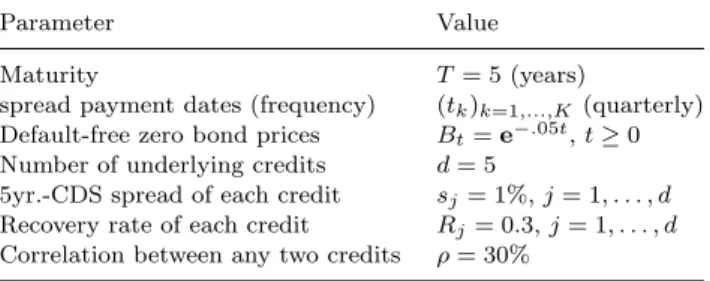
Table 1. Parameters of FTD example; the fair spread of the FTD is 417.88bp.

Parameter Value

Maturity T= 5 (years)

spread payment dates (frequency) (tk)k=1,...,K (quarterly) Default-free zero bond prices Bt=e−.05t,t≥0 Number of underlying credits d= 5

5yr.-CDS spread of each credit sj= 1%,j= 1, . . . , d Recovery rate of each credit Rj= 0.3,j= 1, . . . , d Correlation between any two credits ρ= 30%

The valuation algorithm for the fair FTD spread is given by Algorithm 1. The input parameters for an example involving 5 homogeneous credits are given in Table 1. The fair FTD spread was computed from simulations using random numbers and using low discrepancy sequences, both “as is” and adding a LHSD step. This leads to the following four simulation cases:

(i) Standard Monte Carlo simulation (ii) LHSD based on random numbers

(iii) Simulation with low discrepancy sequence (iv) LHSD based on low discrepancy sequence

The implementation was done in C++ with the QuantLib library [QuantLib (2008)] using the Mersenne twister algorithm for random number generation and Sobol sequences for low discrep-ancy sequences. Root mean square error estimates were obtained by simulating each estimator 100 times. The RMSE estimates and RMSE ratios for various samples sizes are given in Table 2. The ratios of CPU time consumed for generating samples with and without LHSD is also shown for various sample sizes. The CPU time ratios do not include the CPU time required for computing the FTD payoff; consequently the efficiency of LHSD increases with the CPU time required for computing the payoff function. The LHSD step involves sorting a sequence of random numbers (see e.g. [Press et al.(1992)], Chapter 8.4 for sorting algorithms), hence the computational overhead of the LHSD step is of the complexity of the sorting algorithm. On the other hand, by Lemma 22, the rank statistics can be computed from samples of any distribution (cf. Line 13 in Algorithm 1), whereas in a typical Monte Carlo simulation, the generated samples may additionally need to be transformed to uniforms. Finally, observe that over all simulations, LHSD samples a fixed number of default events of the individual credits, but the occurence of joint defaults is random.

Table 2. Root mean square error of estimation in basis points and CPU time ratios for various sample sizes (100 simulations of estimator). Compa-rable ratios were obtained for smaller simulation sizes. The fair FTD spread is 417.88bp. No. of sim. (×103_{) 200 400 600 800 1000} MC 2.02 1.47 1.10 0.89 0.80 MC + LHSD 1.00 0.61 0.53 0.45 0.39 Sobol 0.30 0.20 0.16 0.14 0.11 Sobol + LHSD 0.21 0.12 0.11 0.09 0.08 MC/(MC + LHSD) 2.02 2.41 2.08 1.98 2.05 Sobol/(Sobol + LHSD) 1.43 1.67 1.45 1.56 1.38 CPU time (MC + LHSD)/MC 1.66 1.71 1.75 1.78 1.82 CPU (Sobol + LHSD)/Sobol 1.47 1.52 1.54 1.55 1.56

Note: CPU time ratios involve the generation of random samples only. Adding the CPU time required for computing the payoff decreases the ratios accordingly.

7.2. Example: Valuing an Asian basket option

We now consider pricing an Asian basket optionc_{, whose payoff depends on the sum of several} underlying assets monitored at various points in time. As this is a path-dependent option in a high-dimensional setting, simulation is a standard valuation approach. Following [Imai and Tan (2007)], the payoff may be formulated as a function of a matrix product whose dimensions depend on the number of assets and time points monitored.

Assume a basket ofmassets, withSi

tthe price of thei-th asset at time t,i= 1, . . . , m. Fixing a

maturity T, a strike K, a set of nmonitoring time points 0< t1< t2 < . . . < tn =T and weights wij_{,i= 1, . . . m,j= 1, . . . n,}P

i,jw

ij _{= 1, the payoff of the Asian basket call option on them-asset}

basket is max   m X i=1 n X j=1 wijS_ti j −K,0  . (19)

We assume that asset prices follow a Geometric Brownian motion, i.e.,S1_{, . . . , S}m_{is the solution of}

the stochastic differential equation (SDE)

dS_ti=rS_tidt+σiS_tidW_ti, i= 1, . . . , m,

where r is the risk-free interest rate, σi _{is the volatility of the i-th asset and (W}1_{, . . . , W}m_{) is an} m-dimensional Brownian motion, whose componentsWi,Wk are correlated withρik, 1≤i, k≤m. The solution of the SDE is given by

S_ti=S₀ie(r−(σi)2/2)t+σiWti_{, i= 1, . . . , m. (20)}

Pricing the option requires simulating the paths of each asset at the monitoring time points. Assume that the time points t1, . . . , tn are equidistant and let ∆t =T /nso that tj =j∆t. Let Σ

be anm×mcovariance matrix given by Σ = (ρik_σi_σk_∆t)

i,k=1,...,m. Let ˜Σ be thenm×nm-matrix

generated from Σ via

˜ Σ =      Σ Σ · · · Σ Σ 2Σ· · ·2Σ .. . ... . .. ... Σ 2Σ· · ·nΣ      .

The asset prices may be simulated according to Equation (20) with ˜ W = (σ1Wt11, . . . , σ m_Wm t1, σ 1_W1 t2, . . . , σ m_Wm tn) 0 _{derived via} ˜ W = ˜CZ,

where ˜C is such that ˜CC˜0 = ˜Σ and Z is a vector of nm independent standard Normal random variables. The payoff at time T of the Asian basket option can then be written as

max(g( ˜W)−K,0) with g( ˜W) = mn X k=1 eµk+ ˜Wk µk= ln(wk1k2Sk1(0)) + r−(σ k1₎2_/2t k2, where k1= (k−1) modm+ 1 k2=b(k−1)/mc+ 1, k= 1, . . . , mn.

In this approach, simulation of option payoffs involves the computation of products of high-dimensional matrices. For ˜C we choose the Cholesky decomposition of ˜Σ (i.e., ˜C is lower triangular c_{This is also known as an arithmetic average Asian option.}

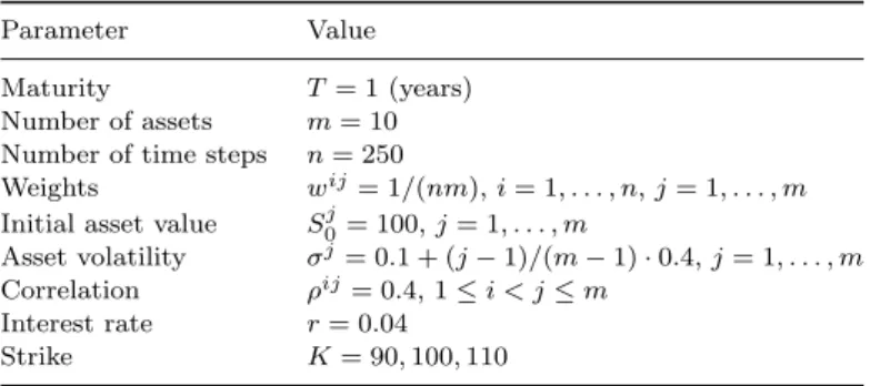
Table 3. Parameters of Asian basket option

Parameter Value

Maturity T= 1 (years)

Number of assets m= 10 Number of time steps n= 250

Weights wij_{= 1/(nm),i= 1, . . . , n,j= 1, . . . , m} Initial asset value S₀j= 100,j= 1, . . . , m

Asset volatility σj_{= 0.1 + (j−1)/(m−1)·0.4,j= 1, . . . , m} Correlation ρij_{= 0.4, 1≤i < j≤m}

Interest rate r= 0.04

Strike K= 90,100,110

Table 4. Simulated prices of an Asian basket option (parameters in Table 3) for strikes K∈ {90,100,110}. The results are based on 10 runs with 4096 and 8192 simulations each. The numbers in parentheses denote the sample standard deviation based on the 10 runs. The CPU time ratios of LHSD versus MC were 1.40 CPU seconds (4096 simulations) and 1.44 CPU seconds (8192 simulations).

sim. size K= 90 K= 100 K= 110 MC 4096 12.3045 (0.1930) 5.6726 (0.1402) 2.0574 (0.0916) MC+LHSD 4096 12.3283 (0.0130) 5.6567 (0.0187) 2.0288 (0.0316) MC 8192 12.3481 (0.1602) 5.6697 (0.1041) 2.0413 (0.0633) MC+LHSD 8192 12.3253 (0.0150) 5.6535 (0.0166) 2.0302 (0.0261) MC/(MC+LHSD) 4096 14.8462 7.4973 2.8987 MC/(MC+LHSD) 8192 10.6800 6.2711 2.4253

with ˜CC˜0= ˜Σ). Typical choices of ˜Cother than the Cholesky decomposition yield a reduction of the dimension of the matrix multiplication, while keeping the error introduced small. For example, the simulation technique of [Imai and Tan (2007)] reduces the dimension of the problem by determining

˜

C as the solution of an optimization problem.

Based on the data set of [Imai and Tan (2007)], we simulate ˜W using a Cholesky decomposition and introducing an LHSD step in each dimension over all simulations. The parameters of the option are given in Table 3. As in [Imai and Tan (2007)], we computed 10 runs of 4096 simulations and 10 runs of 8192 simulations. The resulting prices and standard deviations for Monte Carlo and LHSD are given in Table 4. The implementation was done in C++ usingQuantLib, see [QuantLib (2008)], and using matrix multiplication routines from the Fortran code of GNU Octave, see [GNU Octave (2008)]. The results show that LHSD outperforms the standard Monte Carlo simulator by factors of 2.5 to 15 based on standard deviations (resp. 9 and 200 in terms of variance); the computing time consumed by LHSD increases by a factor of approximately 1.4. The pickup in accuracy depends strongly on the strike of the option and decreases with increasing strike. The same observation is made in an example from [Glasserman (2004), p. 242-243], where an Asian call option is priced using standard LHS. There, this behaviour is attributed to the fact that LHS is more effective the more the function to be estimated is ”additive”; this is resembled at lower strikes, where the option payoffs are more linear.

To benchmark their method, [Imai and Tan (2007)] simulated the Asian basket option using a Quasi-Monte Carlo method together with a technique called Latin supercube sampling. The latter method avoids sampling low discrepancy sequences in high dimensions, see [Owen (1998)]. The standard error of LHSD is comparable to that of the QMC technique, the latter being between 0.00905 and 0.0144. Recall that LHSD is a very simple and practicable technique. Finally, it should be noted that our results do not keep up with standard errors obtained from the dimension reduction technique of [Imai and Tan (2007)], but we conjecture that combinations of LHSD together with dimension-reduction techniques may be effective.

Appendix A. Integration by parts formula

We derive the integration by parts formula as it is used in the paper. An integration by parts formula for two dimensions is given in [Gill et al. (1995)]; a version for_Rk _{is found in [Gill and Johansen}

(1990), p. 1530].

Let us recall some well-known concepts and facts, see e.g. [von Neumann (1950), Chapter X.5]. LetH : [0,1]d→Rbe a right-continuous function. For rectanglesB = (a1, b1]×· · ·×(ad, bd]⊂[0,1]d,

define VH(B) := X cvertex ofB sgn(c)H(c), where sgn(c) = (

1, ifck=ak for an even number ofk’s, −1, ifck=ak for an odd number ofk’s.

If in addition VH(B) ≥ 0 for all rectangles B, then H is called quasi-monotone. If H is

quasi-monotone and right-continuous, it determines a σ-additive, nonnegative measure, which we also denote byH, via

Z

B

dH =VH(B), (A.1)

for all rectangles B. IfH is of bounded variation and right-continuous, then it is the difference of two quasi-monotone, right-continuous functions, and hence determines aσ-additive, signed measure via the relationship (A.1).

Proposition 23. Let H, G: [0,1]4_→

Rbe of bounded variation and right-continuous, with at least

one of H, G continuous and such that RRRR

HdGexists. Then, Z Z Z Z H(u1, u2, u3, u4) dG(u1, u2, u3, u4) = Z Z Z Z VG((u1,1]× · · · ×(u4,1]) dH(u1, u2, u3, u4) + Z Z Z Z H(0, u2, u3, u4) +H(u1,0, u3, u4) +H(u1, u2,0, u4) +H(u1, u2, u3,0) −H(0,0, u3, u4)−H(0, u2,0, u4)−H(0, u2, u3,0) −H(u1,0,0, u4)−H(u1,0, u3,0)−H(u1, u2,0,0) +H(0,0,0, u4) +H(0,0, u3,0) +H(0, u2,0,0) +H(u1,0,0,0) −H(0,0,0,0) dG(u1, u2, u3, u4). (A.2)

Proof. By Equation (A.1),

H(u1, . . . , u4) = Z (0,u1]×···×(0,u4] dH(x1, . . . , x4) +H(0, u2, u3, u4) +H(u1,0, u3, u4) +H(u1, u2,0, u4) +H(u1, u2, u3,0) −H(0,0, u3, u4)−H(0, u2,0, u4)−H(0, u2, u3,0) −H(u1,0,0, u4)−H(u1,0, u3,0)−H(u1, u2,0,0) +H(0,0,0, u4) +H(0,0, u3,0) +H(0, u2,0,0) +H(u1,0,0,0) −H(0,0,0,0).

Insert this expression into Equation (A.2) and apply Fubini’s theorem to the first term, for which we then obtain

Z Z Z Z

The statement follows by observing that from the continuity of one ofH andG, Z (0,1]1_{×···×(0,1]}4 Z (0,1]1_{×···×(0,1]}4 4 X i=1 1_{ui=xi} 4 Y j=1,j6=i 1_{uj≥xj}dG(u1, . . . , u4) dH(x1, . . . , x4) = 0. References

Adams, C. and Clarkson, J. (1934). Properties of functions f(x, y) of bounded variation, Trans. Amer. Math. Soc36, 4, pp. 711–730.

Clarkson, J. and Adams, C. (1933). On definitions of bounded variation for functions of two variables,

Trans. Amer. Math. Soc.35, 4, pp. 824–854.

Deheuvels, P. (1979). La fonction de d´ependance empirique et ses propri´et´es,Bulletin de l’Acad´emie Royale de Belgique, Classe des Sciences 5, 65, pp. 274–292.

Deheuvels, P. (1981). Multivariate tests of independence, in Analytical Methods in Probability Theory, Proceedings of the conference held at Oberwolfach, June 1980, Lecture Notes in Mathematics (Springer), pp. 42–50.

Feller, W. (1971).An Introduction to Probability Theory and Its Applications, Vol. 2, 2nd edn. (John Wiley & Sons, New York).

Fermanian, J.-D., Radulovic, D. and Wegkamp, M. (2004). Weak convergence of empirical copula processes,

Journal of the Bernoulli Society 10, 5, pp. 847–860.

Gaenssler, P. and Stute, W. (1987).Seminar on Empirical Processes, DMV seminar, volume 9 (Birkh¨auser). Genest, C., Ghoudi, K. and Rivest, L.-P. (1995). A semiparametric estimation procedure of dependence parameters in multivariate families of distributions,Biometrika82, 3, pp. 543–552.

Gill, R. and Johansen, S. (1990). A survey of product-integration with a view toward application in survival analysis,Ann. Statist 18, 4, pp. 1501–1555.

Gill, R. D., van der Laan, M. J. and Wellner, J. A. (1995). Inefficient estimators of the bivariate survival function for three models,Ann. Inst. Henri Poincar´e 31, 3, pp. 545–597.

Glasserman, P. (2004).Monte Carlo Methods in Financial Engineering (Springer).

GNU Octave (2008). A high-level language, primarily intended for numerical computations, version 2.9.9, URLhttp://www.octave.org, http://www.octave.org.

Hobson, E. (1921).The Theory of Functions of a Real Variable Vol. I, 2nd edn. (Cambridge University Press).

Imai, J. and Tan, K. S. (2007). A general dimension reduction technique for derivative pricing,Journal of Computational Finance 10, 2, pp. 129–155.

Jacod, J. and Protter, P. (2003).Probability Essentials, 2nd edn. (Springer).

Joe, H. (1997).Multivariate Models and Dependence Concepts(Chapman & Hall/CRC). Kallenberg, O. (2001).Foundations of Modern Probability, 2nd edn. (Springer).

McKay, M. D., Beckman, R. J. and Conover, W. J. (1979). A comparison of three methods for selecting values of input variables in the analysis of output from a computer code,Technometrics 21, pp. 239–245. Nelsen, R. B. (1999).An Introduction to Copulas (Springer).

Owen, A. B. (1992). A central limit theorem for Latin hypercube sampling,Journal of the Royal Statistical Society Series B 54, 13, pp. 541–551.

Owen, A. B. (1998). Latin supercube sampling for very high-dimensional simulations,ACM Transactions on Modeling and Computer Simulation 8, 1, pp. 71–102.

Press, W. H., Teukolsky, S. A., Vetterling, V. and Flannery, B. P. (1992).Numerical Recipes in C: The Art of Scientific Computing, 2nd edn. (Cambridge University Press).

QuantLib (2008). A free/open-source library for quantitative finance, version 0.9.0, URLhttp://quantlib. org, http://quantlib.org.

R¨uschendorf, L. (1976). Asymptotic distributions of multivariate rank order statistics,Ann. Statist.4, 5, pp. 912–923.

Ruymgaart, F. H., Shorack, G. R. and van Zwet, W. R. (1972). Asymptotic normality of nonparametric tests for independence,Annals of Mathematical Statistics 43, 4, pp. 1122–1135.

Schmidt, W. and Ward, I. (2002). Pricing default baskets,RISK 15, 1.

Stein, M. (1987). Large sample properties of simulations using Latin hypercube sampling,Technometrics

29, 2, pp. 143–151, correction in 32:367.

Vaart, A. W. v. d. and Wellner, J. A. (1996).Weak convergence and empirical processes (Springer). von Neumann, J. (1950). Functional operators. Volume I: Measures and integrals (Princeton University Press).