Kent Academic Repository
Full text document (pdf)
Copyright & reuse
Content in the Kent Academic Repository is made available for research purposes. Unless otherwise stated all content is protected by copyright and in the absence of an open licence (eg Creative Commons), permissions for further reuse of content should be sought from the publisher, author or other copyright holder.
Versions of research
The version in the Kent Academic Repository may differ from the final published version.
Users are advised to check http://kar.kent.ac.uk for the status of the paper. Users should always cite the published version of record.
Enquiries
For any further enquiries regarding the licence status of this document, please contact:
If you believe this document infringes copyright then please contact the KAR admin team with the take-down information provided at http://kar.kent.ac.uk/contact.html
Citation for published version
Gong, Bo and Liu, Wenbin and Tang, Tao and Zhao, Weidong and Zhou, Tao (2017) An Efficient
Gradient Projection Method for Stochastic Optimal Control Problems. SIAM Journal on Numerical
Analysis, 55 (6). pp. 2982-3005. ISSN 0036-1429.
DOI
https://doi.org/10.1137/17M1123559
Link to record in KAR
http://kar.kent.ac.uk/65556/
Document Version
Author's Accepted Manuscript
STOCHASTIC OPTIMAL CONTROL PROBLEMS ∗
BO GONG∗, WENBIN LIU†, TAO TANG‡, WEIDONG ZHAO§, AND TAO ZHOU¶
Abstract. In this work, we propose a simple yet effective gradient projection algorithm for a class of stochastic optimal control problems. We first reduce the optimal control problem into an optimization problem for a convex functional by means of a projection operator. Then we propose an convergent iterative scheme for the optimization problem. The key issue in our iterative scheme is to compute the gradient of the objective functional by solving the adjoint equations that are given by backward stochastic differential equations (BSDEs). The Euler method is used to solve the resulting BSDEs. Rigorous convergence analysis is presented and it is shown that the entire numerical algorithm admits a first order rate of convergence. Several numerical examples are carried out to support the theoretical finding.
Key words. Stochastic optimal control, gradient projection methods, backward stochastic differential equations, conditional expectations
AMS subject classifications. 60H35, 65C20, 35Q99, 35R35
1. Introduction. In recent years, stochastic optimal control has been exten-sively studied and has become an essential tool in various fields, such as financial mathematics and engineering. There exists a very extensive body of literature in both theoretical and practical studies of stochastic optimal control problems, see e.g., [4,5,17,25, 8,11] and references therein.
In this work, we are concerned with the following stochastic optimal control prob-lem min u∈KJ(u) =E [ ∫ T 0 ( h(xut) +j ( u(t))) dt+k(xuT) ] , (1.1)
whereuis the control policy, andxuis the corresponding state process that satisfies
the following stochastic differential equation
dxu t =b ( xu t, u(t) ) dt+σ( xu t, u(t) ) dWt, t∈(0, T], x|t=0=x0. (1.2)
Theoretical investigations for the above model can be found in [4,13,17,24,3,7,15,
26,32,36]. For practical applications of (1.1)-(1.2), one can refer to [7,23,26,36,38] for engineering applications, to [21,22, 30,40, 42] for applications in option pricing and portfolio optimization, to [1] for analysis of climate changes, and to [16] for biological and medical problems, to name a few.
In general the above model does not admit explicitly closed form solutions and thus efficient numerical algorithms have been widely studied in recent years. Roughly
∗This work was supported by the National Natural Science Foundations of China under grants
91530118, 11571351, 11171189 and 11571206. The last author is also supported by NCMIS.
∗Department of Mathematics, Hongkong Baptist University, Hongkong, China
†Kent Business School, University of Kent, UK ([email protected])
‡Department of Mathematics, Southern University of Sciences and Technology, Shenzhen, China
§School of Mathematics & Finance Institute, Shandong University, Jinan, China
¶LSEC, Institute of Computational Mathematics, Academy of Mathematics and Systems Science,
Chinese Academy of Sciences, Beijing, China ([email protected]) 1
speaking, we can characterize numerical algorithms into four categories: (i) transfer-ring the control problem into finite dimensional stochastic programming, see e.g., [9, 15, 18, 19, 26, 36, 39, 41]; (ii) dynamic programming principle (DPP) based approach [6, 25]. In this framework, one usually needs to solve the corresponding Hamilton-Bellman-Jacobin (HJB) equations, and this is one of the most widely used numerical methods [2,4,5,10, 20]; (iii) martingale based methods [21, 22,37]; and (iv) stochastic maximum principle (SMP) based methods, see e.g., [17] and references therein.
Basically, the SMP procedure is to directly compute directional derivative for the objective functionalJ(·) by introducing an adjoint process. Then by introducing an optimality condition for the control problem, a variational inequality coupled with the state and adjoint equations forms an optimality condition system (we call it SMP system) that can be used to solve the optimal control problem. While SMP is a popular tool for theoretical studies of stochastic optimal control, see, e.g., [40,42], it has not been widely used in the numerical setting.
In this work, we propose a simple yet effective gradient projection algorithm for the stochastic optimal control problem (1.1)-(1.2). We first reduce the optimal control problem to an optimization problem for a convex functional by means of a projection operator. Then we propose an convergent iterative scheme for the optimization prob-lem. The key idea in our iterative scheme is to compute the gradient of the objective functional in an efficient way, and this is done by solving the adjoint equations that is given by backward stochastic differential equations (BSDEs). Our approach belongs to SMP based approach, and it relies on solving the SMP system in an efficient way. To this end, we propose a simple yet effective Euler-type method for solving the re-sulting BSDEs. Furthermore, we perform a sharp convergence analysis and we show that our numerical method admits a first order rate of convergence. Several numerical examples are presented to support the theoretical founding.
The rest of the paper is organized as follows. In Section 2 we set up the stochastic optimal control problem and provide with some assumptions. The gradient projection method is presented in Section 3. Section 4 is devoted to convergence analysis of the proposed numerical approach. Several numerical experiments are presented to show the effective of the proposed numerical method in Section 5. We finally give some conclusions in Section 6.
2. Problem Setup. For notational simplicity, we shall narrow our discussion to the one dimensional case, however, the whole framework applies easily to multi-dimensional cases. Let (Ω,F,{Ft}06t6T,P) be a complete probability space with
filtration Ft generated by the Brownian motion {Ws}06s6t. HereT is the terminal
time. We denote by U = L2([0, T];R) the space of all square integrable functions x : [0, T] → R, and denote by UF = L2F([0, T]×Ω;R) the space of all adapted stochastic processesx: [0, T]×Ω→Rthat satisfy
E[ ∫ T 0 (xt)2dt ] <+∞.
Let C ⊂ R be a nonempty, convex and closed subset, and we define the following control set K={ u∈U u(t)∈ Ca.e. } .
Note that we have assumed that the control u is deterministic. We remark that a deterministic control can still be useful for future planning as discussed e.g. in
[7,26] for engineering applications, in [9] for financial applications and in [36] for an application in stochastic hybrid systems. Moreover, stochastic control (i.e.,u∈UF) can also be included in our approach and this will be discussed in Section 5 via numerical examples.
Givenu∈K, the controlled state processxu
t is governed by the SDE
dxut =b ( xut, u(t) ) dt+σ( xut, u(t) ) dWt, t∈(0, T], x|t=0=x0∈R. (2.1)
The considered cost functional is given by
J(u) =E [ ∫ T 0 ( h(xut) +j ( u(t))) dt+k(xuT) ] , (2.2)
whereh(·), j(·), k(·) are given functions andxu
t is the solution of (2.1). We now state
our stochastic optimal control problem as follows:
Find u∗∈K such that J(u∗) = min
u∈KJ(u). (2.3)
Throughout the paper, we shall make the following assumption.
Assumption 1.
• The functionsb=b(x, u)andσ=σ(x, u)are continuously differentiable with
respect to xandu, and have bounded derivatives.
• The functionsh, j andkare continuously differentiable, and their derivatives
have at most a linear growth with respect to the underling variables.
Notice that under Assumption1, the solutionxu
t of (2.1) and the cost functional
J(u) are all well defined foru∈K.
3. The gradient projection method. In this section, we will present details of our gradient projection method. For the stochastic optimal control problem (2.1 )-(2.2), it is well known that for the optimal controlu∗ it holds
(J′(u∗), v−u∗)>0, ∀v∈K, (3.1)
where (J′(u), v) is the variation ofJ(u) along the directionv, i.e., forv∈U such that
u+v∈K,we have
(J′(u), v) = lim
ρ↓0
J(u+ρv)−J(u)
ρ . (3.2)
The existence of such derivatives has been discussed in [13, 32,40]. Here we slightly abuse the notation by referringJ′(u),the functional, to the corresponding element in
U, asU is a Hilbert space.
Next, we propose a gradient projection method for solving the optimal condition (3.1). To this end, let∥ · ∥be the norm of U. We define the projection operatorPK:
ω7→PKω as
PKω−ω= min
u∈K∥u−ω∥. (3.3)
Notice that the projection problem (3.3) is equivalent to the inequality
For any positive constantρ, the variational inequality (3.1) is equivalent to the fol-lowing inequality
(
u∗−(u∗−ρJ′(u∗)), v−u∗)
>0, ∀v∈K. (3.5) By the fact of wellposedness of convex optimizations and by comparing the above inequality with the inequality (3.4), we conclude that for the optimal control u∗, it
holds
u∗=PK(u∗−ρJ′(u∗)). (3.6)
That is, the optimal controlu∗ is the fixed point ofP
K(u−ρJ′(u)) on K.
We shall approximate the control u∗ numerically by step functions. To this end,
we introduce the following uniform time partition:
0 =tN0 < tN1 <· · ·< tNN =T, tNn+1−tNn =T /N =: ∆t. (3.7)
We will denote by IN
n the intervals [tNn−1, tNn) for 1 6 n 6 N −1, and by INN the
interval [tN
N−1, tNN]. In the context whereN is fixed, we shall omit the superscriptN
oftN
n. We also define the associated space of piecewise constant functions by
UN = { u∈U|u= N ∑ n=1 αnXIN n a.e., αn∈R } .
LetKN =K∩UN, then it is clear thatKN is also convex and closed. Now, we define
the approximated problem of (2.3) by
J(u∗,N) = min
u∈KN J(u).
Using similar arguments, one can show that
u∗,N =PKN (
u∗,N−ρJ′(u∗,N))
. (3.8)
Based on the above optimal condition, we propose the following fixed-point iteration scheme to get the approximated optimal control
ui+1,N =PKN (
ui,N−ρiJN′ (ui,N)
)
, i= 1,2,· · · , (3.9) where ρi is a positive constant. Notice that in the above equation we have changed
J′(·) intoJ′
N(·),as one cannot computeJ′(·) exactly in general, and thus it is obtained
by numerical approaches. It is clear that J′
N(·) depends on particular numerical
schemes, and we shall discuss the numerical approximation ofJ′
N(·) in later sections.
We will denote the error betweenJ′(·) andJ′
N(·) by ϵN = sup i J′(uN,i)−JN′ (uN,i) . (3.10)
Next, we show in Theorem 1 the convergence property of the iteration scheme (3.9).
Theorem 1. Assume thatJ′(·)is Lipschitz and uniformly monotone aroundu∗
andu∗,N in the sense that there exist positive constantsc andC such that
∥J′(u∗)−J′(v)∥6C∥u∗−v∥, ∀v∈K, ( J′(u∗)−J′(v), u∗−v) >c∥u∗−v∥2, ∀v∈K, ∥J′(u∗,N)−J′(v)∥6C∥u∗,N−v∥, ∀v∈KN, ( J′(u∗,N)−J′(v), u∗,N−v) >c∥u∗,N−v∥2, ∀v∈KN.
Moreover, we assume that ϵN = sup i J′(ui,N)−JN′ (ui,N) →0, N → ∞.
Suppose thatρi is chosen such that0<1−2cρi+ (1 + 2C)ρ2i 6δ2 for some constant
0< δ <1. Then, the iteration scheme (3.9) is convergent, more precisely, we have
∥u∗−ui,N∥ →0. i, N → ∞.
Proof. By (3.8) and (3.9), we have
u∗,N−ui+1,N 2 6u∗,N−ui,N−ρi(J′(u∗,N)−JN′ (ui,N) ) 2 = u∗,N−ui,N 2 −2ρi ( u∗,N−ui,N, J′(u∗,N)−JN′ (ui,N) ) +ρ2i J′(u∗,N)−JN′ (ui,N) 2 .
By the Lipschitz condition and monotonicity property ofJ′(·),we have −2ρi(u∗,N−ui,N, J′(u∗,N)−JN′ (ui,N)
)
=−2ρi(u∗,N−ui,N, J′(u∗,N)−J′(ui,N) +J′(ui,N)−JN′ (ui,N)
) 6−2cρiu∗,N−ui,N 2 +ρ2i u∗,N−ui,N 2 +ϵ2N. Moreover, we have ρ2i J′(u∗,N)−JN′ (ui,N) 2 =ρ2i
J′(u∗,N)−J′(ui,N) +J′(ui,N)−JN′ (ui,N) 2 62Cρ2i u∗,N −ui,N 2 + 2ρ2iϵ2N.
It is easy to show that for sufficiently small ρi, there is a constant 0 < δ <1 such
that 0<1−2cρi+ (1 + 2C)ρ2i 6δ2,then we get
u∗,N−ui+1,N 2 6δ2 u∗,N−ui,N 2 + (1 + 2ρ2 i)ϵ2N, (3.11)
Then, there exists a constantC1 that independent ofN and isuch that u∗,N−ui,N 6δi u∗,N−u0,N +C1ϵN.
Under the assumptionϵN →0, we get
∥u∗,N −ui,N∥ →0. (N, i→ ∞). (3.12) On the other hand, using similar arguments as for deriving (3.11), we obtain
u∗−u∗,N = u∗−PKN(u∗−ρJ′(u∗)) +PKN ( u∗−ρJ′(u∗))−u∗,N 6∥u∗−PKN(u ∗−ρJ′(u∗))∥+√ 1−2cρ+Cρ2 u∗−u∗,N . Letρ=c/C,C2=(1− √ 1−2cρ+Cρ2)−1 ,we have u∗−u∗,N 6C2∥u∗−PKN(u∗−ρJ′(u∗))∥.
Since C is invariant in time, for v ∈ UN, it holds that PKv ∈ UN. Thus we have
PKv ∈KN, and then we have PKv =PKNv. Now, denotingω :=u∗−ρJ′(u∗), we
have u∗−u∗,N 6C2∥u∗−PKN(u ∗−ρJ′(u∗))∥=C 2∥PKω−PKNω∥ 6C2(∥PKω−PKPUNω∥+∥PKPUNω−PKNω∥) =C2(∥PKω−PKPUNω∥+∥PKNPUNω−PKNω∥) 62C2∥ω−PUNω∥.
AsUN is dense inU, we have∥ω−PUNω∥ →0, and thus∥u∗−u∗
,N∥ →0.Then, the
conclusion follows from this argument and (3.12).
In Theorem 1 we have shown the convergence of ∥u∗,N −ui,N∥ under the
as-sumptionϵN →0.Note that this is a reasonable assumption. In fact, under certain
regularity requirements, and by designing suitable numerical approaches for JN′ (·),
one could further expect that ϵN ∼ O(∆t). In such a case, we could expect a first
order rate of convergence of our iteration scheme (3.9), as illustrated in the following corollary.
Corollary 1. Suppose that the conditions in Theorem 1 holds, and furthermore,
we assume thatu∗andJ′(u∗)are both Lipschitz continuous functions inU, then under
the conditionϵN ∼O(∆t) we have
u∗−ui,N
∼ O(∆t), i→ ∞.
The iteration scheme (3.9) is the starting point of our numerical approach for stochas-tic optimal control problems. In the following sections, we shall show how to get the numerical approximationJ′
N(u) ofJ′(u) in each iteration.
3.1. The representation ofJ′(u). It is noticed that the iteration scheme (3.9)
involves the computation of J′(u). In this section, we will derive a new formula of
J′(u) for fixed u ∈ K by introducing a pair of adjoint processes. Again in all our
arguments,J′(u) is referred to the element of U.
By the definition (3.2), we have (J′(u), v) = lim ρ↓0 J(u+ρv)−J(u) ρ =E[ ∫ T 0 h′(xu t)Dxut(v)dt+ ∫ T 0 j′( u(t)) v(t)dt+k′(xu T)DxuT(v) ] , (3.13) wherexu
t is the solution of the SDE (2.1), and
Dxut(v) := lim ρ↓0
xut+ρv−xut
ρ .
Under Assumption1, the processDxu
t(v) satisfies the SDE
dDxut(v) = ( b′x ( xut, u(t) ) Dxut(v) +b′u ( xut, u(t) ) v(t))dt +(σx′ ( xut, u(t) ) Dxut(v) +σu′ ( xut, u(t) ) v(t))dWt, Dxu0(v) = 0. (3.14)
Notice that one can resort to the above equation to getJ′(u), however, this would
this, we shall introduce a pair of adjoint processes (pu, qu) that solves the following
backward stochastic differential equation (BSDE):
−dput =f ( xut, put, qtu, u(t) ) dt−qutdWt, puT =g(xuT) =k′(xuT), (3.15) wheref is defined as f(x, p, q, u) =h′(x) +p b′ x(x, u) +q σ′x(x, u).
Notice that by the standard BSDE theory, under Assumption 1, the BSDE (3.15) admits an unique solution (pu
t, qut) foru∈K. We remark that theoretical studies of
BSDEs has been a hot topic recently. In particular, the wellposedness of our adjoint equation, i.e., the BSDEs (3.15), has been well discussed under mild assumptions. One can refer to [34,33,29] for more details on the BSDEs theory.
We shall show in the following that by introducing the pair (pu
t, qut), the involving
termsDxu
t(v) in (3.13) will be canceled. More precisely, by Itˇo’s formula, we have
h′(xut)Dxut(v)dt =−Dxut(v)dput − ( put b′x ( xut, u(t) ) +qut σx′ ( xut, u(t) )) Dxut(v)dt+qutDxut(v)dWt =−d( putDxut(v) ) +putdDxut(v) +qtu ( σ′x ( xut, u(t) ) Dxut(v) +σu′ ( xut, u(t) ) v(t))dt −(putb′x ( xut, u(t) ) +qutσ′x ( xut, u(t) )) Dxtu(v)dt+qtuDxut(v)dWt =−d( putDxut(v) ) +(putb′u ( xut, u(t) ) +qtuσ′u ( xut, u(t) )) v(t)dt +(putσ′x ( xut, u(t) ) Dxut(v) +putσu′ ( xut, u(t) ) v(t) +qtuDxut(v) ) dWt. (3.16)
Then, by inserting (3.16) into (3.13), we obtain (J′(u), v) = ∫ T 0 ( E[putb′u ( xut, u(t) ) +qutσu′ ( xut, u(t) )] +j′( u(t))) v(t)dt.
Then, we can re-defineJ′(u) by
J′(u)|t=E[putb′u ( xut, u(t) ) +qut σu′ ( xut, u(t) )] +j′( u(t)) . (3.17) HereJ′(u)|trepresentsJ′(u), as an element ofU, valued att.
To simplify the expression ofJ′(u),we have introduced a pair of adjoint processes
(pu, qu) that satisfies the BSDE (3.15), to get rid of the termDxu
t(·). Then, by solving
the BSDE (3.15), we can get the solution pair (pu, qu) numerically, and then further
get an approximated J′
N(u) of J′(u) by using (3.17). In the next section, we shall
propose an Euler type method for solving the adjoint BSDE (3.15).
Remark 1. We remark that the authors in [12] also introduced an adjoint
e-quation to cancel the term Dxu
t(·). The adjoint equation therein is an anticipating
integrand stochastic differential equation, where the solution is required to be backward-adapted instead of the classic forward backward-adapted. However, such a requirement is not
true in general. In other words, the wellposedness of the adjoint equation in [12] is
3.2. Numerical approximations for adjoint equations. By (3.15), it is no-ticed that the solution pair (pu
t, qtu) depends on the forward process xut. Hence, we
need to solve (for t ∈ [0, T]) the following forward-backward stochastic differential equations (FBSDEs) { dxu t =b ( xu t, u(t) ) dt+σ( xu t, u(t) ) dWt, xt=0=x0, −dpu t =f ( xu t, put, qtu, u(t) ) dt−qu tdWt, puT =g(xuT). (3.18) Next, we shall discuss how to solve the above FBSDEs numerically with a given
u∈K.For notation simplicity, we shall omit the superscript uin this section, such asxt=xut, pt=put,qt=qtu.
Under mild assumptions, it is well known that the above backward equation is wellposed [35]. Moreover, the solutionsptandqthave the representations
pt=η(t, xt), qt=σ(xt, u(t))∂xη(t, xt), (3.19)
whereη(t, x) : [0, T]×R→Ris the solution of the following parabolic PDE
L0η(t, x) =−f(x, η(t, x), σ( x, u(t)) ∂xη(t, x), u(t) ) , η(T, x) =g(x), (3.20) with L0η(t, x) =∂tη(t, x) +b(x, u(t))∂xη(t, x) + 1 2σ ( x, u(t))2∂xxη(t, x),
The representations in (3.19) is the so called nonlinear Feynman-Kac formula [35]. We remark that numerical methods for FBSDEs is a hot topic recently, and one can refer to [27,28,44,45,46] and references therein for variable numerical approaches. Here in this paper, we shall introduce a simple scheme, namely the Euler scheme, for solving the FBSDEs (3.18).
3.3. The Euler scheme for FBSDEs. We now follow closely the work [45] and [46] to introduce the Euler method for solving the FBSDEs (3.18). The time partition was defined in (3.7). By integrating both sides of the backward equation on [tn, tn+1] we obtain ptn =ptn+1+ ∫ tn+1 tn f(xt, pt, qt, u(t))dt− ∫ tn+1 tn qtdWt. (3.21)
Then by taking conditional expectation Extn[·] = E[·| Ftn, xtn =x] on both sides of
(3.21) and applying the left-point rectangular rule, we have
pxtn=E x tn [ ptn+1 ] + ∆t f( x, pxtn, q x tn, u(tn) ) + ¯Rxp,n, (3.22) where ¯ Rxp,n= ∫ tn+1 tn Extn [ f( xt, pt, qt, u(t))]dt−∆t f(x, pxtn, q x tn, u(tn) )
is the truncation error due to the left-point rectangular rule. Equation (3.22) is our reference equation for solvingp.
Next, we aim to deriving another reference equation for solving q. To this end, by multiplying (3.21) by ∆Wn+1:=Wtn+1−Wtn and taking conditional expectation
Extn[·] on both sides of the derived equation and then applying again the left-point
rectangular rule, we obtain
qxtn= 1 ∆t ( Extn [ ptn+1∆Wn+1 ] + ¯Rxq,n ) , (3.23) where ¯ Rx q,n= ∫ tn+1 tn Extn [ f( xt, pt, qt, u(t))∆Wn+1]dt− ∫ tn+1 tn Extn[qt]dt+ ∆t q x tn
is again the corresponding truncation error. By removing the error terms ¯Rx
p,n and ¯Rxq,n in (3.22) and (3.23), we get the
following semi-discretization scheme for the BSDE in (3.18): impose the initial value of px
N =g(x) on x∈R, and then for n=N−1,· · · ,1,0, compute pxn =pn(x) and
qx
n=qn(x) withx∈Rin a backward way by
pxn=Extn [ pn+1]+ ∆t f(x, pxn, qxn, u(tn)), (3.24) qxn= 1 ∆tE x tn [ pn+1∆Wn+1]. (3.25)
Notice that in the above semi-discretization schemes (3.24) and (3.25), solvingpx nand
qx
nfor eachx∈Rmay involve the knowledge ofpn+1on the whole space regionR. To
apply this scheme into practice, the spacial discretization ofRand the approximations of the conditional expectationExtn[·] are required.
To do this, we introduce a uniform partitionRh of theRas
Rh={xk
k= 0,±1,±2, ... }
, with ∆x=xk+1−xk.
We shall denote Ik =: [xk, xk+1]. Notice that the above partition involves infinite
grid points, however, this is unnecessary in practical applications, as we are always interested in the final information (t = 0) in a finite interval. This means that we can consider a finite partition with |k| ≤P with P being a positive integer (which can be very large and problem dependent). In what follows, we shall consider a finite partition with the parameterP.We remark that how to choose a reasonableP is not a trivial work, and we refer to [46] for further discussions.
On the partitionRh, we introduce a continuous piece-wise linear function space
Vh, the element of whichv∈Vh can be represented as follows
v(x) = ∑ |k|≤P vk(xk)ϕk(x), with ϕk(x) = x−xk−1 xk−xk−1, x∈Ik−1, xk+1−x xk+1−xk, x∈Ik, 0, otherwise.
For a continuous functionf(x), we now introduce the associated interpolation oper-atorIhby
Ihf(x) =
∑
|k|≤P
f(xk)ϕk(x),
3.3.1. The approximation of conditional expectations. We now discuss the approximation of conditional expectations. Let ˜xtn,x
tn+1 be the Euler approximation
of the statextn,x tn+1, namely, ˜ xtn,x tn+1=x+b ( x, u(tn))∆t+σ(x, u(tn))∆Wn+1 =x+b( x, u(tn))∆t+σ(x, u(tn)) √ ∆t ζ, (3.26)
whereζ∼ N(0,1) is a normal random variable. We choose ˜ptn,x tn+1 = ptn+1(˜x tn,x tn+1) = η(tn+1,x˜ tn,x tn+1) to approximate p tn,x tn+1, where η(t, x) is the solution of the problem (3.19). As a result, ˜ptn,xk
tn+1 is a function of ˜x
tn,xk
tn+1,
thus a function of the increment ∆Wn+1. Therefore, the conditional expectation
Extn[˜ptn+1] (as well as E
x
tn[˜ptn+1∆Wn+1]) can be written into an integral on R with
the Gaussian probability density function ρ(ξ) = √1
2πe
−ξ2/2
. Hence we propose the Gauss-Hermite quadrature rule to approximate these conditional expectations. The
L-point Gauss-Hermite quadrature rule for a functionf writes
E[f(ζ)] = ∫ R f(ξ)ρ(ξ)dξ≈ L ∑ ℓ=1 f(ξℓ)ωℓ, (3.27)
where{ξℓ}and{ωℓ}are the Gaussian-Hermite quadrature points and the associated
weights, respectively.
Consider for example the approximation of the conditional expectationExtn[˜ptn+1],
we have Extn[˜ptn+1] =E[ptn+1(˜x tn,x tn+1)] =E[ ptn+1 ( x+b( x, u(tn))∆t+σ(x, u(tn)) √ ∆t ζ)] ≈ L ∑ ℓ=1 ptn+1 ( x+b( x, u(tn))∆t+σ(x, u(tn)) √ ∆t ξℓ)ωℓ. (3.28)
We shall denote by ˜Extn[ptn+1] the approximation ofE
x tn[˜ptn+1], more precisely, ˜ Extn[ptn+1] = L ∑ ℓ=1 ptn+1 ( x+b( x, u(tn))∆t+σ(x, u(tn)) √ ∆t ξℓ)ωℓ. (3.29)
Similarly we denote by ˜Extn[ptn+1∆Wn+1] the approximation ofE
x tn[˜ptn+1∆Wn+1] : ˜ Extn[ptn+1∆Wn+1] = L ∑ ℓ=1 ptn+1 ( x+b( x, u(tn))∆t+σ(x, u(tn)) √ ∆t ξℓ) √ ∆t ξℓωℓ. (3.30) In the quadrature rule (3.29), it is noticed that ˆx=x+b(x, u(tn))∆t+σ(x, u(tn))
√
∆t ξℓ
may not be on the partitionRh. Therefore, we shall resort to the linear interpolation
Ih to get the desired information. To this end, we define
ˆ Extn[ptn+1] = L ∑ ℓ=1 Ihptn+1 ( x+b( x, u(tn))∆t+σ(x, u(tn)) √ ∆t ξℓ)ωℓ. (3.31)
Similarly, we define ˆExtn[ptn+1∆Wn+1] as ˆ Extn[ptn+1∆Wn+1] = L ∑ ℓ=1 Ihptn+1 ( x+b( x, u(tn))∆t +σ( x, u(tn)) √ ∆t ξℓ) √ ∆t ξℓωℓ. (3.32)
Notice that the approximated expectation ˆExtn[·] is a function of x.In the partition
spaceRh, we denote ˆEtn[·] := ˆE
xtn
tn [·]. In addition, for functionsf ∈Vh, we have
ˆ Extn[f(˜x tn,x tn+1)] = ˜E x tn[f(˜x tn,x tn+1)], ˆ Extn[f(˜x tn,x tn+1)∆Wn+1] = ˜E x tn[f(˜x tn,x tn+1)∆Wn+1].
Based on the above observations, we finally get the following approximations ˆExtn[ptn+1]
and ˆExtn[ptn+1∆Wn+1] of E x tn[ptn+1] andE x tn[ptn+1∆Wn+1] : Extn[ptn+1] = ˆE x tn[ptn+1] + ˆR x p,n, Extn[ptn+1∆Wn+1] = ˆE x tn[ptn+1∆Wn+1] + ˆR x q,n, (3.33) where ˆRk
p,nand ˆRkq,nare the truncation errors:
ˆ Rxp,n= ˜Rp,nx +RxE,p,n+RxIh,p,n, ˆ Rxq,n= ˜Rq,nx +RxE,q,n+RxIh,q,n, (3.34) with ˜ Rxp,n=Extn[ptn+1]−E x tn[˜ptn+1], R˜ x q,n=Extn[ptn+1∆Wn+1]−E x tn[˜ptn+1∆Wn+1], RxE,p,n=Extn[˜ptn+1]−E˜ x tn[ptn+1], R x E,q,n=Extn[˜ptn+1∆Wn+1]−E˜ x tn[ptn+1∆Wn+1], RxIh,p,n= ˜E x tn[ptn+1]−Eˆ x tn[ptn+1], R x Ih,q,n = ˜E x tn[ptn+1∆Wn+1]−Eˆ x tn[ptn+1∆Wn+1].
3.3.2. The fully discrete scheme. By the reference equations (3.22) and (3.23) and the approximations of the conditional expectations in (3.31), we get the following two equations: pxtn= ˆE x tn [ ptn+1 ] + ∆t f( x, pxtn, q x tn, u(tn) ) +Rxp,n, pxtN =g(x), (3.35) qtxn= 1 ∆t ( ˆ Extn [ ptn+1∆Wn+1 ] +Rxq,n ) , (3.36) whereRx
p,nandRxq,nare the total truncation errors defined by
Rxp,n= ¯Rxp,n+ ˆRxp,n, Rxq,n= ¯Rq,nx + ˆRxq,n (3.37)
with ¯Rx
p,n and ¯Rxq,ndefined in (3.22) and (3.23), and ˆRxp,nand ˆRq,nx defined in (3.34).
Based on the two reference equations (3.35) and (3.36), we propose a fully dis-crete numerical scheme for solving the FBSDEs (3.18) as follows: given the terminal conditionpN =∑|k|≤Pg(xk)ϕk(·)∈Vh, forn=N−1,· · · ,1,0, and each xk ∈Rh,
solvepn∈Vh andqn∈Vh by pkn= ˆEx k tn [ pn+1 ] + ∆t f( xk, pkn, qnk, u(tn) ) , (3.38) qnk = 1 ∆tEˆ xk tn [ pn+1∆Wn+1]. (3.39)
3.4. Summary of the numerical approach. We now summarize the entire algorithm of our gradient projection method. In the fixed-point iteration (3.9), we have introduced J′
N(·) as the approximation of J′(·). As the relation between J′(·)
and the adjoint processes (p, q) has been revealed in (3.17), it is natural to define the approximationJ′
N(·) by replacingp,qandE[·] in (3.17) with the numerical ones.
More precisely, we define
J′ N(u)|tn = ˆE [ pnb′u ( ·, u(tn))+qnσu′ ( ·, u(tn))]+j′(u(tn)), (3.40) where ˆE[·] is defined by ˆ E[ϕt0] =ϕt0, Eˆ[ϕtn] = ˆE x0 t0[ˆEt1[· · ·Eˆtn−1[ϕtn]]], n>1. (3.41)
To make sure thatJ′
N(·)∈UN, we define JN′ (u)|t= N−1 ∑ n=0 JN′ (u)|tnXInN(t). (3.42)
Then, the gradient projection method is summarized in Algorithm1.
Algorithm 1Gradient projection method
Set the initial guess of the controlu0∈UN and the error toleranceϵ0;
1. Set the terminal condition: pk
N =g(xk),xk∈Rh;
2. Forn=N−1,· · · ,1,0, solve (pn, qn) by (3.38)-(3.39);
3. ComputeJ′
N(u)|tn by (3.40);
4. Updateuby (3.9);
Repeat the above steps until the error∥ui+1,N
−ui,N
∥reaches the toleranceϵ0.
4. Error estimates. In this section, we shall perform a rigorous error analysis for our gradient projection method. As concluded in Corollary 1, the first order rate of convergence relies on the estimate ϵN = O(∆t). By observing the definition of
(3.17) and (3.40), we see that the error ϵN contains two parts: the numerical error
of (pk
n, qnk) and the approximation error of ˆE[·]. In the following sections, we shall
estimate the two parts one by one.
4.1. Preliminary results of the discrete operator Eˆ[·]. In this subsection, we first show some basic properties of the approximated conditional expectations ˆ
Exk
tn[·] and ˆE[·] which are defined in (3.31) and (3.41) respectively.
Notice that the weights of the quadrature rule {ωℓ} are all positive and there
holds
∑
ℓ
ωℓ= 1.
Moreover, the L-point Gauss-Hermite quadrature rule is exact for polynomials with degree less than or equal to 2L−1. We now state some basic properties of ˆExk
tn[·] in
the following:
Proposition 1. Given variablesϕt
n+1 = ¯ϕ(tn+1, xtn+1), for L>2, we have
• Eˆ[ˆEtn[ϕtn+1]] = ˆE[ϕtn+1].
• If for any x, it holdsϕx
tn+1 >0,then we have
ˆ
Exk
• (Eˆxk tn[ϕtn+1] )2 6Eˆxk tn[(ϕtn+1) 2], (ˆE[ϕ tn]) 26Eˆ[(ϕ tn) 2], ( ˆ Exk tn[ϕtn+1∆Wtn+1] )2 6 ( ˆ Exk tn[(ϕtn+1) 2] −(ˆExk tn[ϕtn+1]) 2)∆t.
The above propositions are all well known and easy to prove. It is also known that under Assumption 1, form>1 it holds that
E[|xt|m]6C(|x0|m+ 1).
In the following, we shall provide a similar result for the approximated expectation ˆ
E[·]. Notice that in what follows,C shall stand for a constant that is independent of ∆t, ∆x,nandk, while its value may vary from place to place.
Proposition 2. Under Assumption 1, for m>2, L>2, and∆x=O(√∆t), it holds
ˆ
E[|xtn|
m]6C(
|x0|m+ 1).
Proof. We denote byIh|x|m the linear interpolation of the function| · |m at x.
By the interpolation theory, there exists θ ∈[x−, x+] (where x− < x+ are two grid points aroundx) such that for ∆xsufficiently small, it holds
Ih|x|m6|x|m+ 1 8m(m−1)|θ| m−2(∆x)2 6|x|m+1 8m(m−1) ( (|x|+ ∆x)m+ 1) (∆x)2 6|x|m+C( |x|m+C∆x( |x|m+ 1) + 1) (∆x)2 6(1 +C(∆x)2) |x|m+C(∆x)2. (4.1) For fixed k and ℓ, let a1 = xk +b(xk, u(tn))∆t and a2 = σ(xk, u(tn))√∆t ξℓ, then
there existsθ∈[a1, a1+a2] such that
|xk,ℓ|m=|a1+a2|m=|a1|m+m|a1|m−1sgn(a1)a2+m(m−1)|θ|m−2(a2)2
6|a1|m+m|a1|m−1sgn(a1)a2+m(m−1)(|a1|+|a2|)m−2(a2)2. (4.2)
By the assumptions onbandσ, for sufficiently small ∆twe have
|a1|m6((1 +C∆t)|xk|+C∆t) m
6(1 +C∆t)m|xk|m+C∆t(|xk|m+ 1)
6(1 +C∆t)|xk|m+C∆t,
|a1|+|a2|6C(|xk|+ 1).
Using together (4.1)-(4.2) and the definition
xk,ℓ=xk+b(xk, u(tn))∆t+σ(xk, u(tn))
√
we have ˆ Exk tn[|xtn+1| m] = L ∑ ℓ=1 Ih|xk,ℓ|mωℓ 6(1 +C(∆x)2) L ∑ ℓ=1 |xk,ℓ|mωℓ+C(∆x)2 6(1 +C(∆x)2)( (1 +C∆t)|xk|m+C∆t+C(|xk|m+ 1)∆t ) +C(∆x)2 6(1 +C(∆x)2)( (1 +C∆t)|xk|m+C∆t)+C(∆x)2.
Consequently, by the definition (3.41) and the assumption ∆x=O(√∆t), we have ˆ E[ |xtn+1| m] = ˆE[ˆ Etn[|xtn+1| m]] 6(1 +C(∆x)2)( (1 +C∆t)ˆE[|xtn| m] +C∆t)+C(∆x)2 6(1 +C(∆x)2)n+1 (1 +C∆t)n+1( |x0|m+ (n+ 1)C∆t+ (n+ 1)C(∆x)2 ) 6C(|x0|m+ 1).
This completes the proof.
Next, by the variational arguments, we can easily present an approximation prop-erty for the expectation ˆE[·].
Lemma 1. Assume thatb, σ ∈C0,4
b . For ϕt= ¯ϕ(t, xt)with ϕ¯ ∈Cb0,4, we define
Φti(x) =E
x
ti[ϕtn],then it holdsΦti∈C 0,4
b , and furthermore, we have
E[ϕtn] = ˆE[ϕtn] + n−1 ∑ i=0 ˆ E[ ˆRΦ,i], with RˆΦ,i=E xti ti [Φti+1]−Eˆ xti ti [Φti+1], 16i6n.
4.2. The error estimates of(pk
n, qnk). We let
µn=ptn−pn, νn=qtn−qn,
where (pt, qt) and (pn, qn) are the exact solutions of the FBSDEs (3.18) and numerical
solutions of the scheme (3.38)-(3.39), respectively. Notice that
pn(x) = ∞ ∑ k=−∞ pknϕk(x), qn(x) = ∞ ∑ k=−∞ qnkϕk(x), where (pk
n, qkn) are numerical solutions by scheme (3.38)-(3.39), and forxk ∈Rh we
have (pk n, qnk) = (pn(xk), qn(xk)).We now define µkn=p xk tn −p k n, νnk=q xk tn −q k n.
Then, by subtracting the equation (3.38) from the equation (3.35), and the equation (3.39) from the equation (3.36), respectively, we deduce that
µkn = ˆE xk tn[µn+1] + ∆t δf k n+Rkp,n, µkN =p xk tN −p k N, (4.3) νnk= 1 ∆t ( ˆ Exk tn[µn+1∆Wn+1] +R k q,n ) , (4.4)
where δfnk=f(xk, pxtnk, q xk tn, u(tn))−f(xk, p k n, qnk, u(tn)), Rkp,n=Rx k p,n, Rq,nk =Rx k q,n.
Now, we are ready to give the estimates of µk
n and νnk in the following Lemma.
The estimates also imply the stability of the scheme (3.38)-(3.39) and will be used in our final error estimates.
Lemma 2. Under proposition 1, namely, assume that f(x, p, q, u) is Lipschitz
continuous with respect topandq, uniformly in xandu, then there holds
ˆ E[(µn)2] + ∆t N−1 ∑ n=0 ˆ E[(νn)2]6CEˆ[(µN)2] + C ∆t N−1 ∑ n=0 ˆ E[(Rp,n)2+ (Rq,n)2].
Proof. By taking square of the equations (4.3)-(4.4), and using together
Proposi-tion1, and the inequality (a+b)26(1 +ϵ)a2+ (1 + 1/ϵ)b2 we get
(µkn)26(1 +γ∆t) (ˆ Exk tn[µn+1] )2 , +C(1 + 1 γ∆t )( ∆t2( (µkn)2+ (νnk)2 ) + (Rp,nk )2 ) (νk n)26 C ∆t ( ˆ Exk tn[(µn+1) 2] −(ˆ Exk tn[µn+1] )2) + C (∆t)2 ( Rk q,n )2 .
Let ∆t61/γ,γ= 4C2, and add up the above inequalities to get
(µk n)2+ ∆t 2C(ν k n)26(1 +γ∆t)ˆEx k tn[(µn+1) 2] + ∆t 2C(µ k n)2 + 1 2∆t ( (Rk p,n)2+ (Rkq,n)2 ) , which yields (µk n)2+C∆t(νnk)26(1 +C∆t)ˆEx k tn[(µn+1) 2] + 1 ∆t ( (Rk p,n)2+ (Rkq,n)2 ) .
By taking discrete expectation on the above inequality, using together property i, we have ˆ E[(µn)2] +C∆tEˆ[(νn)2]6(1 +C∆t)ˆE[(µn+1)2] + 1 ∆tEˆ [ (Rp,n)2+ (Rq,n)2]. (4.5) Then, we gets ˆ E[(µn)2]6CEˆ[(µN)2] + C ∆t N−1 ∑ n=0 ˆ E[ (Rp,n)2+ (Rq,n)2]. (4.6)
Taking the summation of (4.5) fromn= 0 toN−1 we get
C∆t N−1 ∑ n=0 ˆ E[(νn)2]6 N−1 ∑ n=0 ( C∆tEˆ[(µn+1)2] + 1 ∆tEˆ [ (Rp,n)2+ (Rq,n)2] ) 6CEˆ[(µN)2] + C ∆t N−1 ∑ n=0 ˆ E[ (Rp,n)2+ (Rq,n)2]. (4.7)
Then, the proof is completed.
We now provide with the following lemma for estimating the truncation errors, and the proof is somehow standard using the arguments of approximation theory.
Lemma 3. Suppose that Assumptions 1 holds, and moreover, we assume that
b(·, w), σ(·, w) ∈ C4 b, and f(·,·,·, w) ∈ C 2,2,2 b hold uniformly in w ∈ C, η ∈ C 1,4 b . Then, we have 1 ∆t N−1 ∑ n=0 ˆ E[ (Rp,n)2+ (Rq,n)2]=O((∆t)2)+O((∆x)4/(∆t)2).
Proof. As shown in (3.34), (3.35) and (3.36),Rk
p,nandRkq,nconsist of the following
parts of errors.
Rkp,n= ¯Rkp,n+ ˜Rkp,n+RkE,p,n+RkIh,p,n, Rkq,n= ¯Rkq,n+ ˜Rkq,n+RkE,q,n+RkIh,q,n.
(4.8) By the interpolation theory, we have the following estimate
RkIh,p,n=O (
(∆x)2), RkIh,q,n=O (
(∆x)2).
Also, by the error estimate of the Gauss quadrature rule [31], forf ∈Crand 0< ϵ <1
we have 1 √ 2π ∫ R f(ξ)e−ξ2/2dξ− L ∑ ℓ=1 f(ξℓ)ωℓ 6CL −r/2 √ 2π ∫ R| f(r)(ξ)e−(1−ϵ)ξ2/2|dξ,
where the constant C is dependents onr while independent ofL andf. Therefore, we have that RkE,p,n 6Cσ ( xk, u(tn) )4 (∆t)2, RkE,q,n 6Cσ ( xk, u(tn) )4 (∆t)5/2+Cσ( xk, u(tn) )3 (∆t)2.
Then, by Proposition2, we have ˆ
E[(RE,p,n)2] =O((∆t)4), Eˆ[(RE,q,n)2] =O((∆t)4).
For ˜Rk
p,nand ˜Rkq,n, a rough estimation follows by the Taylor expansion: by subtracting
(4.10) from (4.9) we obtain Exk tn[ptn+1] =p xk tn+1+ ∆tLη(tn+1, xk) + ∫ tn+1 tn ∫ s tn Exk tn[LLη(tn+1, yr)]drds, (4.9) Exk tn[˜ptn+1] =p xk tn+1+ ∆tLη(tn+1, xk) + ∫ tn+1 tn ∫ s tn Exk tn[LLη(tn+1,y˜r)]drds, (4.10)
then we can deduce that ˜Rk p,n=O ( (∆t)2) , where Lη(t, x) =b( x, u(t)) ∂xη(t, x) + 1 2σ ( x, u(t))2∂xxη(t, x).
Similarly, for ˜Rk
q,n we can derive that ˜Rkq,n = O
(
(∆t)2)
. Finally, for the semi-discretization error, we have
¯ Rxk p,n= ∫ tn+1 tn ∫ t tn Exk tn[L 0f¯(s, y s)]dsdt, ¯ Rxk q,n= ∫ tn+1 tn ∫ t tn Exk tn[L 0f¯(s, y s)∆Wn+1+L1f¯(s, ys)− L0ζ(s, ys)]dsdt, where ¯f(t, x) =f( x, η(t, x), ζ(t, x), u(t))
. Thus, by recalling thatu∈UN, we have
¯ Rxk p,n=O ( (∆t)2) , R¯xk q,n=O ( (∆t)2) .
Then, the desired result follows by combining all the estimates above.
Using together the above arguments (Lemma 1-3), we can finally get the following error estimates for our numerical schemes:
Theorem 2. Suppose that assumption 1 holds, and under similar assumptions
as in the above lemmas. Then, the conclusions of Lemma2and Lemma3imply
ˆ E[(µn)2] + ∆t N−1 ∑ n=0 ˆ E[ (νn)2]=O((∆t)2)+O((∆x)4/(∆t)2).
Then, we can further get
ϵN = sup i ∥J ′(uN,i) −JN′ (uN,i)∥=O(∆t) +O ( (∆x)2/∆t) .
In particular, by taking ∆x= ∆t, we have that ϵN =O(∆t). Then, using together
Corollary 1, we have
∥u∗−uN,i
∥=O(∆t), i→ ∞.
Proof. Givenu∈UN, we define
ϕt=ptb′u ( xt, u(t))+qtσ′u ( xt, u(t))+j′(u(t)), ϕkn=pknb′u ( xk, u(tn))+qknσ′u ( xk, u(tn))+j′(u(tn)).
ϕt= ¯ϕ(t, xt). Moreover,J′(u)|t=E[ϕt],JN′ (u)|tn= ˆE[ϕn]. Then, we have ∥J′(u)−J′ N(u)∥2 6C N−1 ∑ n=0 ∫ tn+1 tn ( J′(u)|t−J′(u)|tn )2 +( J′(u)|tn−J ′ N(u)|tn )2 dt =C N−1 ∑ n=0 ∫ tn+1 tn (∫ t tn d drE[ϕr] r=sds )2 dt +C∆t N−1 ∑ n=0 ( E[ϕtn]−Eˆ[ϕn] )2 6C∆t N−1 ∑ n=0 ∫ tn+1 tn ∫ t tn ( E[L0ϕ¯(s, y s)] )2 ds dt +C∆t N−1 ∑ n=0 (( E[ϕtn]−Eˆ[ϕtn] )2 +(ˆ E[ϕtn]−Eˆ[ϕn] )2) 6C(∆t)2+C(∆x)4/(∆t)2+C∆t N−1 ∑ n=0 ˆ E[ (µn)2+ (νn)2] =O( (∆t)2) +O( (∆x)4/(∆t)2) .
Notice that the above estimation of∥J′(u)−J′
N(u)∥2 does not depend on the choice
ofu,and then, we complete the proof.
5. Numerical experiments. In this section, we present several numerical ex-amples to verify the efficiency of our numerical approach. In all our computations, we need to choose a reasonable parameter ρ. Motivated by the error estimates in the last section, it is noticed that the scheme admits good convergence property with sufficiently smallρ. However, extremely smallρwould decrease the convergence rate of the iteration. In our examples, we shall simply choose ρi = 1/
√
i. And in what follows, we shall denote by ”CT” the convergence rate.
Example 1. Our first example has been used in [12]. The optimal control problem
is stated as
J(u∗) = min
u∈KJ(u)
with the cost functional
J(u) = 1 2 ∫ T 0 E[( xt−x∗(t) )2] dt+1 2 ∫ T 0 u2(t)dt, K=U,
and the controlled state equation
dxt=u(t)xtdt+σxtdWt.
Here σ is a constant. The deterministic function x∗ and the corresponding exact
solutionu∗ are given by
u∗(t) = T−t 1 x0 − T t+t 2 2 , x∗(t) = eσ 2t −(T−t)2 1 x0− T t+t 2 2 + 1. (5.1)
We setx0= 1,T = 1 andσ= 0.1, and the number of samples for approximating the
expectation is chosen asM = 105, and we set the tolerance asϵ
0= 10−5. Numerical
t 0 0.2 0.4 0.6 0.8 1 control 0 0.2 0.4 0.6 0.8 1
1.2 exact solution and numerical solution exact numerical log(N) 1.6 1.7 1.8 1.9 2 log(error) -3.1 -3 -2.9 -2.8 -2.7 -2.6 -2.5 convergence rate error 1st order rate
Fig. 1.Numerical results for example 1 with solution (5.1).
The left plot shows that the numerical solution matches the exact solution very well when N = 100. In the right plot, we have tested the error decays with N = 40,50,· · · ,100, and it is clearly shown that the method admits a first order rate of convergence.
Next, we test a different pair (x∗, u∗) which is given by
u∗(t) = e− T −e−t 1 x0 + 1−e−t−te−T , x∗(t) = e σ2 t −(e−T −e−t)2 1 x0 + 1−e−t−te−T − e−t. (5.2) We setσ= 0.1,M = 105,ϵ
0= 10−5 andN = 40,50,· · ·,100. The numerical results
are given in Figure2. Again, the numerical solution matches the exact solution very well and first order convergence rate is observed.
t 0 0.2 0.4 0.6 0.8 1 control -0.7 -0.6 -0.5 -0.4 -0.3 -0.2 -0.1
0 exact solution and numerical solution exact numerical log(N) 1.6 1.7 1.8 1.9 2 log(error) -3.7 -3.65 -3.6 -3.55 -3.5 -3.45 -3.4 -3.35 -3.3 -3.25 -3.2 convergence rate error 1st order rate
Fig. 2.Numerical results for example 1 with solution (5.2).
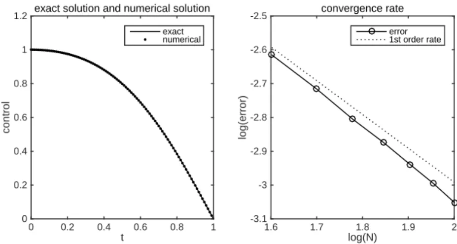
Example 2. Our second example is also from [12]. More precisely, we consider
J(u∗) = min
with J(u) = 1 2 ∫ T 0 E[( xt−x∗(t) )2] dt+1 2 ∫ T 0 u2(t)dt, K=U, dxt=(u(t)−r(t))dt+σu(t)dWt. Here we set r(t) =u∗(t)/2, x
0 = 0, T = 1, andσ is a constant. The deterministic
functionx∗ and the corresponding exact solutionu∗ are chosen as
u∗(t) = T−t σ2(T−t) + 1, x∗(t) = t 2σ2 − 1 2σ4ln σ2T+ 1 σ2(T −t) + 1+ 1.
In our computations, we chooseσ= 0.1,M = 105,ϵ
0= 10−5, andN = 40,50,· · ·,100.
The numerical results are shown in Figure 3Similar conclusions can be made as for example 1. The method converge with the first order accuracy.
t 0 0.2 0.4 0.6 0.8 1 control 0 0.1 0.2 0.3 0.4 0.5 0.6 0.7 0.8 0.9
1 exact solution and numerical solution exact numerical log(N) 1.6 1.7 1.8 1.9 2 log(error) -3.3 -3.25 -3.2 -3.15 -3.1 -3.05 -3 -2.95 -2.9 -2.85 -2.8 convergence rate error 1st order rate
Fig. 3. Numerical results for example 2.
Example 3. The previous discussions have been focused on the deterministic
con-trol, that is,u∈U. In this example, we will show that our method can also be used to solve stochastic optimal control problems with feed back control.
This example is set to be the same as in (2.1)-(2.2), except that the control constraint set is now a set of stochastic controls:
KF ={u∈UF
ut(ω)∈ Ca.e. a.s.}. (5.3)
It follows from the stochastic optimal control theory that the optimal control is actually a feedback control, more precisely, there exists a function ¯u∗ such that
u∗
t = ¯u∗(t, xt), see e.g. [43, 14]. Given a feedback control u with ut = ¯u(t, xt),
by introducing the adjoint processes (p, q) in the same way as in the deterministic case, and by applying the Itˇo’s formula, we can show that
J′(u)
t=ptb′u(xt, ut) +qtσ′u(xt, ut) +j′(ut). (5.4)
Notice thatut is a function oft and xt, then by (5.4) we know thatJ′(u)t is also a
function oft andxt. Therefore, due to the feedback property of the control, we can
writeJ′(u) pointwisely in time-space grids, namely,
J′(u)x tn=p x tnb ′ u ( x,u¯(tn, x))+qtxnσ ′ u ( x,u¯(tn, x))+j′(u¯(tn, x)), (5.5)
where x∈ Dh and J′(u)xt denotes J′(u)t valued at xt = x. In the above equation,
by introdcing our numerical solutions pn and qn, we get the approximatedJN′ (·) of
J′(·) : JN′ (u)kn =pknb′u ( xk,u¯(tn, xk))+qknσu′ ( xk,u¯(tn, xk))+j′(u¯(tn, xk)). (5.6)
Since the constraintK(5.3) is also pointwise in time and space, the projection problem at the grid point (tn, x),x∈Dh can be written as
¯
u∗(tn, x) =PC(¯u∗(tn, x)−ρJ′(u∗)xtn )
.
Here we shall not compute the feedback law explicitly, however, we do compute the values of the control at the grid point. Thenu∗ is updated in the following way:
¯
ui+1(t
n, xk) =PC(u¯i(tn, xk)−ρiJN′ (ui)kn
)
. (5.7)
Notice that due to the change of the space of control, we get rid of the expectation in the computation of J′(u), meaning that we no longer need the history
informa-tion before time t to compute J′(u)
t, but only the information at time instance t.
Consequently, if a proper space partition {xk}k is obtained, and the constraintK is
pointwise in time, then we can run the algorithm in a backward manner as described in Algorithm 2. Compared to Algorithm 1, we notice that under the same spacial
Algorithm 2Gradient projection method
Set the initial guess of the control{u¯(tn, xk)}n,k and the error tolerance ϵ0;
1. Set the terminal condition: pk
N =g(xk),xk∈Rh;
2. Forn=N−1,· · · ,1,0, do a. solve (pn, qn) by (3.38)-(3.39),
b. computeJN′ (u)kn by (5.6),
c. updateuby (5.7),
repeat a–c until supk|u¯i+1(tn, xk)−u¯i(tn, xk)| ≤ϵ0.
partition, Algorithm 2 can save a lot restoration.
We now test Algorithm 2 for Example 3 with K defined in (5.3), and compare the results using feedback control with the results obtained by using the deterministic control. For the feedback control, we shall use the rectangular rule and Monte Carlo method to compute the integral and the expectation of objective functional, respec-tively. The numerical results are listed in the Table 1. It is shown that the use of feedback control can indeed improve the results (produces a smaller value of objec-tive functional), and this is reasonable as we are minimizing the objecobjec-tive functional within a larger control set.
N J(u) with Algorithm 1 J(u) with Alogrithm 2
100 0.84833 0.62535
200 0.84797 0.64507
400 0.84777 0.65509
800 0.84770 0.66013
Table 1
Example 4. Our last example is a portfolio problem. We consider the following example which has been used in [9].
J(u∗) = min u∈KJ(u) with J(u) = 1 2E [ (xT −κ)2], K={u∈UF; −16ut61, a.e. a.s.}, dxt= (ζσut+r)xtdt+σutxtdWt.
The parameters are chosen as
T = 50, κ= 1000, x0= 300, r= 0.02, σ= 0.1, ζ= 0.05.
We setϵ0 = 10−4, L= 4, ρi = 0.01/i, and the space region is given by [−100,900].
The optimal value of J(u) given in [9] is 15023. To show the convergence rate, we perform experiments withN = 1000,2000,4000,8000, and choose M =N2/10. The
corresponding numerical solutions for J(u) are listed in the Table 2. It is clear that the method admits a first order rate of convergence. This example shows that the Algorithm 2 is capable of solving some optimal control problems involving feedback control.
N 1000 2000 4000 8000 optimal
J(u) 15196 15107 15069 15045 15023 CR - 1.0423 0.8688 1.0641
Table 2
Numerical results for example 5.4.
6. Conclusion. In this work, we propose a gradient projection method for solv-ing stochastic optimal control problems. The scheme contains a fixed-point iteration of the control, and an Euler scheme for solving the adjoint equation that is given by BSDEs. The Euler method is used to solve the adjoint BSDEs. We rigorously prove that our numerical method admits a first order rate of convergence. Several numerical tests are presented to support our theoretical finding.
REFERENCES
[1] O. Bahn, A. Haurie, and R. Malhame. A stochastic control model for optimal timing of climate policies. Automatica, 44(6): 1545-1558, 2008.
[2] M. Bardi and I. Capuzzo-Dolcetta, Optimal control and viscosity solutions of Hamilton-Jacobi-Bellman equations, Birkh¨auser, Boston, 1997.
[3] K. Barty, J.-S. Roy, and C. Strugarek. A stochastic gradient type algorithm for closed-loop problems. Mathematical Progamming, 119(1): 51-78, 2009.
[4] A. Bensoussan, Lecture on Stochastic Control, in Nonlinear Filtering and Stochastic Control, Lecture Notes in Mathematics 972, Proc. Cortona, Springer-Verlag, Berlin, New York, 1981. [5] A. Bensoussan, Stochastic Control by Functional Analysis Methods, North-Holland Publishing
Company, New York, 1982.
[6] D.P. Bertsekas, Dynamic programming and optimal control, vol. II. Athena Scientific, 2007. [7] F. Campillo, J. Nekkachi, and E. Pardoux, Numerical methods in ergodic stochastic control,
application to semi active vehicle suspensions, In Proceedings of the 29th IEEE conference on Decision and Control, Honolulu, 1990.
[8] P. Carpentier, G. Cohen, and A. Dallagi, Particle Methods for Stochastic Optimal Control Problems, Computational Optimization and Applications, 56: 635-674, 2013..
[9] J. Chen, Some Problems of Optimal Control and the Application in Financial Mathematics, Master’s Thesis, Tongji University, China, 2007.
[10] M. Crandall and P. L. Lions, Viscosity solutions of Hamilton-Jacobi equations, Trans. Amer. Math. Soc., 277 (1983), 1-42.
[11] A. Dallagi, M´ethodes particulaires en commande optimale stochastique. Th`ese de doctorat, Universit´e Paris 1, Panth´eon-Sorbonne, 2007.
[12] N. Du, J.T. Shi, and W.B. Liu, An effective gradient projection method for stochastic optimal control, International Journal of Numerical Analysis and Modeling, 4(2013), pp. 757-774. [13] R.J. Elliott, The Optimal Control of Diffusions, Applied Mathematics and Optimization, Vol.
22, pp. 229-240, 1990.
[14] W.H. Fleming and R.W. Rishel, Deterministic and Stochastic Optimal Control, Spring, New York, 2012.
[15] P. Girardeau, A comparison of sample-based stochastic optimal control methods, Mathematics, 2010.
[16] F.B. Hanson, Applied stochastic processes and control for Jump-diffusions: modeling, analysis, and computation. SIAM, 2007.
[17] U.G. Haussmann, Some examples of optimal stochastic controls or: the stochastic maximum principle at work. SIAM Review, 23(3): 292-307, 1981.
[18] H. Heitsch, and W. Romisch, Scenario Reduction Algorithms in Stochastic Programming. Com-putational Optimization and Applications, 24: 187-206, 2003.
[19] H. Heitsch, W. Romisch, and C. Strugarek, Stability of multistage stochastic programs. SIAM Journal on Optimization, 17: 511-525, 2006.
[20] C.S. Huang, S. Wang, and K.L. Teo, Solving Hamilton-Jacobi-Bellman Equations by a Modified Method of Characteristics, Nonlinear Analysis, Theory, Methods and Applications, Vol. 40, 2000, 279-293.
[21] R. Korn, Optimal Portfolios: Stochastic Models for Optimal Investment and Risk Management in Continuous Time, World ScientificSingapore, 1997.
[22] R. Korn, and H. Kraft, A stochastic control approach to portfolio problems with stochastic interest rates, SIAM Journal on Control and Optimization, Vol.40, No.4, 2001, 1250-1269. [23] D. Kuhn, P. Parpas, and B. Rustem. Stochastic optimization of investment planning problems
in the electric power industry, in Process Systems Engineering: Volume 5: Energy Systems Engineering, 2008.
[24] H.J. Kushner, Necessary Conditions for Continuous Parameter Stochastic Optimization Prob-lems, SIAM Journal on Control, Vol. 10, pp. 550-565, 1972.
[25] H.J. Kushner and P. Dupuis, Numerical methods for stochastic control problems in continuous time. 2nd ed., Springer-Verlag, New York, 2001.
[26] A. Li, E.M. Feng, and X.L. Sun, Stochastic optimal control and algorithm of the trajectory of horizontal wells, Journal of Computational and Applied Mathematics, vol. 212, no. 2, 2008, 419-430.
[27] J. P. Lemor, E. Gobet, and X. Warin, A regression-base monte carlo method for backward stochastic differential equations, Ann. Appl. Probab., 15 (2005).
[28] G. N. Milstein and M. V. Tretyakov, Numerical algorithms for forward-backward stochastic differential equations, SIAM J. Sci. Comput., 28 (2006), pp. 561-582.
[29] J. Ma and Jiongmin Yong, Forward-Backward Stochastic Differential Equations and their Ap-plications, Springer, 2007.
[30] R.C. Merton, Continuous-Time Finance. Blackwell, Cambridge, Massachusetts, 1992.
[31] Mastroianni G, Monegato G. Error estimates for Gauss-Laguerre and Gauss-Hermite quadrature formulas, Approximation and Computation: A Festschrift in Honor of Walter Gautschi. Birkhuser Boston, 1994: 421-434.
[32] S.G. Peng, A general stochastic maximum principle for optimal control problems, SIAM J. Control Optim., 28(4)(1990), 966-979.
[33] E. Pardoux and S. Peng, Adapted solution of a backword stochastic differential equaion, Systems Control Lett., 14(1990), pp. 55-61.
[34] S.G. Peng, Backward Stochastic Differential Equations and Applications to Optimal Control, Appl. Math Optim., 27(1993), 125-144.
[35] S.G. Peng, Probabilistic interpretation for systems of quasilinear parabolic partial differential equations, Stochastics Stochastics Reps., 37(1991), pp. 61-74.
[36] R. Raffard, J. Hu, and C. Tomlin, Adjoint-based optimal control of the expected exit time for stochastic hybrid systems, in M. Morari, L. Thiele (Eds.): Hybrid Systems: Computation and Control 2005, LNCS 3414, Springer-Verlag, 557-572, 2005.
[37] L.C.G. Rogers, Pathwise Stochastic Optimal Control. SIAM Journal on Control and Optimiza-tion, 46(3): 1116-1132, 2007.
[38] S.P. Sethi and Q. Zhang. Hierarchical decision making in stochastic manufacturing systems. Birkhauser Verlag, Basel, Switzerland, 1994.
[39] A. Shapiro and A. Ruszczynski, (Eds.): Stochastic Programming. Elsevier, Amsterdam, 2003. [40] J.T. Shi and Z. Wu, A Stochastic Maximum Principle for Optimal Control of Jump
Diffu-sions and Applications to Finance, Chinese Journal of Applied Probability and Statistics, 27(2011), 127-137.
[41] J.C. Spall, Stochastic Optimization II.6, in Handbook of Computational Statistics (J. Gentle, W. H¨ardle, and Y. Mori, eds.), Springer-Verlag, New York, 2004, 169-197.
[42] W.S. Xu, Maximum Principle for a Stochastic Optimal Control Problem and Application to Portfolio/Consumption Choice, Journal of optimization theory and applications: Vol. 98, No. 3, pp. 719-731, 1998.
[43] J. Yong and X.Y. Zhou, Stochastic Controls: Hamiltonian Systems and HJB Equations, Springer, New York, 1999.
[44] T. Tang, W. Zhao, and T. Zhou, Deferred Correction Methods for Forward Backward Stochastic Differential Equations, Numer. Math. Theor. Meth. Appl., 10(2), pp.222-242, 2017. [45] W. Zhao, L. Chen, and S. Peng, A new kind of accurate numerical method for backward
stochastic differential equations, SIAM J. Sci. Comput., 28 (2006), pp. 1563-1581.
[46] W. Zhao, Y. Fu, and T. Zhou, New kinds of high-order multistep schemes for coupled forward backward stochastic differential equations, SIAM J. Sci. Comput., 36 (2014), pp. A1731-A1751.
[47] W. Zhao, T. Zhou, and T. Kong, High order numerical schemes for second order FBSDEs with applications to stochastic optimal control, Commun. Comput. Phys., (21)2017, pp. 808-834.