This is a repository copy of
Deep learning to filter SMS spam
.
White Rose Research Online URL for this paper:
http://eprints.whiterose.ac.uk/150578/
Version: Accepted Version
Article:
Roy, Pradeep Kumar, Singh, Jyoti Prakash and Banerjee, Snehasish
orcid.org/0000-0001-6355-0470 (2020) Deep learning to filter SMS spam. Future
generation computer systems. pp. 524-533. ISSN 0167-739X
Reuse
This article is distributed under the terms of the Creative Commons Attribution-NonCommercial-NoDerivs (CC BY-NC-ND) licence. This licence only allows you to download this work and share it with others as long as you credit the authors, but you can’t change the article in any way or use it commercially. More
information and the full terms of the licence here: https://creativecommons.org/licenses/ Takedown
If you consider content in White Rose Research Online to be in breach of UK law, please notify us by
Deep Learning to Filter SMS Spam
Pradeep Kumar Roya,b,∗, Jyoti Prakash Singhc, Snehasish Banerjeed
aVellore Institute of Technology, Vellore, India
bMadanapalle Institute of Technology and Science, Madanapalle, Chittoor, India cNational Institute of Technology Patna, India
dThe York Management School, University of York, Freboys Lane, Heslington, York YO10 5GD
Abstract
The popularity of short message service (SMS) has been growing over the last decade. For businesses, these text messages are more effective than even emails. This is because while 98% of mobile users read their SMS by the end of the day, about 80% of the emails remain unopened. The popularity of SMS has also given rise to SMS Spam, which refers to any irrelevant text messages delivered using mobile networks. They are severely annoying to users. Most existing research that has attempted to filter SMS Spam has relied on manually identified features. Extending the current literature, this paper uses deep learning to classify Spam and Not-Spam text messages. Specifically, Convolutional Neural Network and Long Short-term memory models were employed. The proposed models were based on text data only, and self-extracted the feature set. On a benchmark dataset consisting of 747 Spam and 4,827 Not-Spam text messages, a remarkable accuracy of99.44%was achieved.
Keywords: Spam detection; SMS; Machine learning; Deep learning; Convolutional Neural Network; LSTM
1. Introduction
People are increasingly using mobile text messages as a way of communication. The popularity of short message service (SMS) has been growing over the last decade. The volume of SMS sent per month on average has increased by a whopping 7700% from 2008 to 2018. For businesses, text messages are more effective than even emails. This is because while 98% of mobile users read their SMS by the end of the day, about 80% of the emails remain unopened (SMS Comparison, 2018) (SMS, 2018). Hence, it is easy to understand why SMS has grown into a multi-billion dollar commercial industry (Almeida et al., 2011).
Unfortunately, over the years, mobile phones have also become the target for what is known as SMS Spam. SMS Spam refers to any irrelevant text messages delivered using mobile networks. They are severely annoying to users (Almeida et al., 2011; Wang et al., 2010). An example of an annoying spam text message is as follows (Yamakami, 2003; Gupta et al., 2019; Chen et al., 2018)“CONGRATS: YOUR MOBILE NO HAVE WON YOU £500,000 IN
——-∗I am corresponding author
Email addresses:[email protected](Pradeep Kumar Roy),[email protected](Jyoti Prakash Singh),
[email protected](Snehasish Banerjee)
MOBILE DRAW UK, TO CLAIM PRIZE SEND BANK DETAIL, NAME, ADDRESS, MOBILE NO, SEX, AGE, TO –. Such messages come not only from domestic but also international senders. A survey revealed that 68% of mobile phone users are affected by SMS Spam, with teenagers being the worst affected community1.
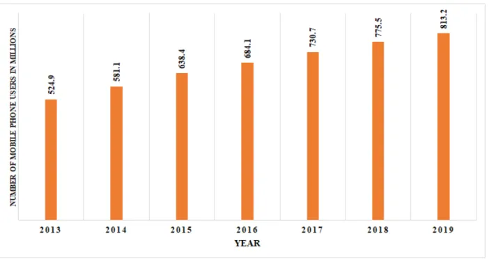
SMS Spam has become popular due to variety of reasons. For one, the cost of sending SMS has decreased dramatically and has even become zero in some cases. In addition, the mobile phone user-base is continually growing. The number of mobile phone users in countries such as India have increased to 775 million in 2018 and by following the patterns it may reach 813 million by 2019 as shown in Figure Figure 12.
Figure 1: The statistics of Mobile Phone users in India
Moreover, unlike emails that are supported with sophisticated spam filtering (Androutsopoulos et al., 2000; Drucker et al., 1999), SMS spam filtering is still not very robust. This is because most works that classify SMS spam (Chen et al., 2015, 2018; El-Alfy & AlHasan, 2016; Fu et al., 2014; Gupta et al., 2019; Kim et al., 2015; Osho et al., 2014) suffer from the limitation of manual feature engineering, which is not an efficient approach. Identifying prospective features for accurate classification requires prior knowledge and domain expertise. Even then, the selec-tion of the features needs to be reassessed based on criteria such as informaselec-tion gain and feature importance graph. Only then, it is possible to identify features that are helpful for the classification, and those that are not. Such an iterative trial-and-error process is expectedly time-consuming (Jain et al., 2019; Nguyen et al., 2017; Saumya et al., 2019).
One way to obviate this inefficient feature engineering process lies in the use of deep neural networks. Deep
1https://www.tatango.com/blog/text-message-spam-infographic/[Accessed on 30th November, 2018]
learning is a class of machine learning techniques in which several layers of information processing stages are ex-ploited for automatic pattern classification as well as unsupervised feature learning (Jain et al., 2019; Kumar & Singh, 2019). The components of a deep neural network work together to self-train itself iteratively in order to minimize classification errors. Over the years, deep neural network based architecture such as Convolutional Neural Network (Kalchbrenner et al., 2014), Recurrent Neural Network (Pascanu et al., 2013), Long Short-Term Memory (Hochreiter & Schmidhuber, 1997; Fischer & Krauss, 2018; Xia et al., 2018) and their variations have been shown to be helpful in obviating manual feature engineering. These networks have been successfully adopted in various research domains such as speech recognition (Dahl et al., 2012; Palaz et al., 2019), sentence modeling (Bengio et al., 2003; Gu et al., 2018; Yin et al., 2016), and image processing (Krizhevsky et al., 2012; Shang & Zhang, 2016; Zhang et al., 2019). However, deep neural networks have not yet been applied in the classification of SMS Spam.
To address the research gap, this paper seeks to harness the strength of deep neural networks for classifying SMS Spam. It leverages the Convolutional Neural Network (CNN) model. This is because CNN is helpful to capture local and temporal features including n-grams from texts (Kalchbrenner et al., 2014; Saumya et al., 2019). Another deep neural network called the Recurrent Neural Network (RNN) was deemed to be useful. This is because RNN is equipped to handle the long-term dependency of word sequences (Pascanu et al., 2013). By parsing just a few initial words of a message, RNN can determine if it is Spam or Not-Spam. The ability of RNN to remember long sequences of text could be useful because SMS do not necessarily have any length restrictions. Nonetheless, the standard RNN suffers from the vanishing gradient problem. Hence, a variant of RNN known as LSTM was used (Fischer & Krauss, 2018; Xia et al., 2018). After all, previous related research has also utilized LSTM (Jiang et al., 2018; Lee & Dernoncourt, 2016; Zhou et al., 2015).
Therefore, the objective of this paper is to classify mobile text messages as Spam or Not-Spam using the CNN and the LSTM model. Our main contributions are:
• We propose a deep learning based framework to classify SMS Spam.
• The proposed model outperforms traditional machine learning classifiers on balanced and imbalanced dataset, achieving a remarkable accuracy of99.44%.
The rest of the paper is organized as follows: Section 2 is the literature review, Section 3 is the proposed method-ology. In section 4, we discuss the detailed experimental setting along with their results. Section 5 discusses the theoretical and practical implications of the proposed model. The conclusion is presented in Section 6.
2. Literature Review
Over the years, computer scientists have proposed several machine learning models to separate Spam from Not-Spam (Abdullahi et al., 2016; AlaM et al., 2018; Chen et al., 2017; Cohen et al., 2018; Chan et al., 2015; Faulkner, 1997; Hancock, 2001; Hinde, 2002; Jeong et al., 2016; Lai, 2007; Li et al., 2017; Vorakulpipat et al., 2012; Wang &
Chen, 2007). These works are not only limited to mobile phone text messages but also include Web Spam (Makkar & Kumar, 2019), Email Spam (Androutsopoulos et al., 2000; Drucker et al., 1999), and Spam on social network platforms such as Facebook, Twitter, and Sina Weibo (Ahmed et al., 2015; Chen et al., 2017; Fu et al., 2018; Lee et al., 2010; Liu et al., 2017).
Jindal & Liu (2007) proposed a model to filter Spam and categorize them into different Spam categories on product advertising blogs. However, they did not consider the SMS Spam category. More recently, (Jiang et al., 2016) classified unfaithful messages into four categories called traditional spam, fake reviews, social spam and link farming. However, their taxonomy also failed to cover SMS Spam. It would seem that research on SMS Spam is relatively limited compared with that on other forms of Spam.
Delany et al. (2012) provided a survey of existing works for filtering Spam SMS. They mostly covered articles that relied on traditional machine learning approaches but not deep learning. For example, (Mathew & Issac, 2011) compared Bayesian classifier with other classification algorithms and found that the former was better to classify Spam text messages. They used the WEKA tool (Hall et al., 2009) for their implementation in which string texts are not accepted. Hence, they had to convert the text messages into the vector form using the WEKA function called StringToWordVector before employing the Bayesian classifier. Almeida et al. (2011) used the SVM classifier to classify Spam texts. They used word frequency as features, and found SVM to yield promising performance. Rafique et al. (2011) proposed the SLAVE framework (structural algorithm in vague environment) for real-time Spam detection. Their model divided the messages into different bytes such as 7-Byte, 8-Byte, and 16-Byte message and then used the 10-fold cross-validation technique. The model achieved a precision of 0.93 for the Spam class.
Another work on Spam classification of text messages used k-Nearest Neighbor (kNN) and SVM classifiers (Uysal et al., 2013). The messages were converted into the vector form using different permutations of the Bag of Words (BoW). The experimental results confirmed that the combination of the BoW features along with structural features performed better to classify Spam messages. Uysal et al. (2012) proposed another model using the Bayesian classifier. Their model achieved a good precision and recall value to predict spam on a large Spam and Not-Spam dataset. Androulidakis et al. (2013) proposed another model to filter Spam messages. Their model was based on the Android operating system in which the users mobile phone control was used to filter the Spam. The model checked the information of message senders against a predefined spammer list. So, when a message came from the users present in the list of spammers, it was treated as Spam; else Not-Spam. Zainal et al. (2015) proposed a model based on Bayesian classifier. They used the RapidMiner and WEKA tools for their implementation, and found both the tools to be comparable in predicting the Spam and Not-Spam messages.
Of late, researchers have started to use deep neural networks such as CNN (Popovac et al., 2018), and LSTM model (Barushka & Hajek, 2018; Jain et al., 2019) for spam filtering. Popovac et al. (2018) proposed a CNN-based architecture with one layer of convolution and pooling to filter SMS spam. They achieved an accuracy of 98.4%. Jain et al. (2019) used LSTM network (a variant of recurrent neural network) to filter SMS spam. With the help of 6000 features and 200 LSTM nodes, their model achieved an accuracy of 99.01%. They also used three different word
embedding techniques: i) Word2Vec, ii) WordNet, and iii) ConcepNet. For every input word, their model searches the word vectors in these embedding which leads to huge system overload or processing. Another deep neural network based model was proposed by (Barushka & Hajek, 2018). Using various machine learning based algorithms such as NB, RF, SVM, Voting, Adaboost and deep learning based models such as CNN, their proposed model achieved an accuracy of 98.51%. This paper extends these related works by achieving an even higher accuracy of 99.44%, as shown in Section 4.
3. Proposed Methodology
We discuss the traditional machine learning approaches in Section 3.1, the CNN model in section 3.2, the LSTM model in Section 3.3, and hyper-parameter tuning as well as training in Section 3.4.
3.1. Traditional Machine Learning Approach
We needed to identify some features from SMS to be used as input to the machine learning model. We used a supervised model for this work. The following features were extracted from the text: “Nouns, Adjectives, Verbs, Difficult Words, Fletch Reading Score, Dale Challe Score, Length, Set length, Stop Words, Total Words, Wrong Words, Entropy, One Letter Words, Two letter Words and Longer Letter Words”. A detailed description of the selected features are explained below:
• Noun: The number of nouns present in the message.
• Adjective: The number of adjective present in the message.
• Verb: The number of verbs present in the message
• Difficult Words: The words that are not understandable by an American fifth-grade student are known as difficult words.
• Flesh Reading Score: FRE : 206 : 835−(1 : 015∗AS L)−(84 : 6∗AS W) where ASL is average sentence length in words and ASW is the average syllables per word. FRE score lies between 0 and 100 with 0 being very confusing and 100 being easy to read.
• Dale Challe Score: Dale Challe formula uses a set of 3000 words that American fourth-grade students are familiar with, and any word outside that set is considered difficult.
• Stop Words: Stop words are the words which occurs very frequently in English text used such as “the”, “a”, “am” etc. The number of stop words present in the message is counted.
• Total Words: The total number of words present in the message are counted.
• Wrong Words: The words with wrong spelling are called as wrong words. The number of wrong words are counted.
• Entropy: The entropy of the message define the information content of the message
• One Letter Words: The number of one letter words present in the message are counted.
• Two Letter Words: The number of two-letter words present in the message are counted.
• Longer Letter Words: The words which are longer than 3 alphabets are called as longer letter word.
These features are used to classify the message into Spam and Not-Spam classes using classifiers such as i) Naive Bayes (NB), ii) Random Forest (RF), iii) Gradient Boosting (GB), iv) Logistic Regression (LR), and v) Stochastic Gradient Descent (SGD) Classifier. The detail experimental results are discussed in section 4.
3.2. Convolutional Neural Network (CNN)
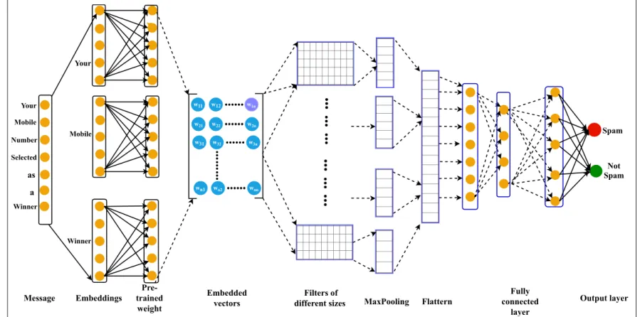
The feature extraction in machine learning based models are manual which required domain knowledge. The accuracy of the classifiers are highly dependent on these features. Deep learning eliminates the need of these manual feature extraction by identifying the hidden features from the data. CNN is one of the popular deep learning models which is able to extract the relevant features from the data . A CNN based model is given in Figure 2 CNN mainly works in three phases: i) the creation of word matrix, ii) identifying the hidden features from the text, and iii) classify them into predefined classes.
Creation of word matrix:Every messageMis the sequence of the words:w1,w2,w3, ,wn. From the given dataset, all unique word are bagged together to create a vocabulary (V) set. Each word of the V is assigned a unique inte-ger value. From the pre-trained word vector called Glove (Pennington et al., 2014), the word vector is extracted for every word present in theV, the word which is not present in the Glove are assigned a default word vector called un-known (UNK). The word vector extracted from the Glove is represented as:E(m)=e(w1),e(w2),e(w3), ,e(wn), where e(w1),e(w2),e(w3), ,e(wn) are the individual word vectors of the wordsw1,w2,w3, ,wn. Finally, the word vectors e(w1),e(w2),e(w3), ,e(wn) are concatenated to create a complete SMS word matrix.
M=e(w1)·e(w2)·e(w3)·e(wn) (1)
where.is the sign of concatenation. In general the SMS word matrix is represented asM1:nfor the messages of the
word 1 to n. In this way an SMS word matrixM∈Rd×|n|is created from every SMS.
M= w11 w12 w13 . . . w1d w21 w22 w23 . . . w2d . . . . . . . . . . . . . . . wn1 wn2 wn3 . . . wnd (2)
w11 w12 w1n w21 w22 w2n w31 w32 w3n wn1 wn2 wnn Your Mobile Number Selected as a Winner
Embeddings trainedPre weight
Embedded
vectors different sizes Filters of MaxPooling Flattern connectedFully layer Output layer Message Your Winner Mobile Spam Not Spam Figure 2: A Frame w ork of Con v olutional Neural Netw ork 7
Context dependent feature extraction phase: A CNN network consists of a series of convolution and pooling layers. For convolution we have used different sizes of kernels: F ∈ 2,3,4,5 (i.e., 2-grams, 3-grams, 4-grams and 5-grams). A convolution operation over the SMS matrixM∈Rd×|n|and kernel F,F∈Rd×|m|(where m=2 is the region
size of the kernel anddis the dimension) yields a feature matrix of dimension (|n| −Fm+1) The process of finding the feature vector is show below:
M= w11 w12 w13 . . . w1d w21 w22 w23 . . . w2d . . . . . . . . . . . . . . . wn1 wn2 wn3 . . . wnd ⊙ Fm= f m11 f m21 f m12 f m22 . . . . . . f m1d f m2d
Where⊙is the convolution operator.
The left matrixMis the message matrix having thennumber of messages with each message havingdword size. Initially, the message are of different sizes as some of the messages have more number of words and some of them have fewer. However, the CNN network does not accept the inputs having different lengths. Therefore, before creating the message matrix (M), we used the post padding technique to make the messages of equal length. The right matrix is the (Fm) is the 2-gram kernel which slides vertically over the message matrix (M) and finds the featuresOi. The featuresOiis calculated as follows:
WhereO1=w11f m11+w12f m12+· · ·+w1df m1d+w21f m21+w22f m22+· · ·+w2df m2d O2=w21f11+w22f12+· · ·+w2df m1d+w31f m21+w32f m22+· · · ·+w3df m2d and
On=w(n−1)1f m11+w(n−1)2f m12+· · ·+wn1f m21+wn2f m22+· · · ·+wndf m2d
These features were stored in a matrixK, the dimension of the matrixKis (n−2+1)×1 the featuresO1,O2,O3, .On are of context-dependent features extracted using the convolution operation.
C= O1 O2 . . . On
The feature matrix K is passed through an activation function called Rectified linear unit (ReLU) (Radford et al., 2015) ReLU is defined as follows (Equation 3).
σ(u)=max(0,u) (3)
The resulting values are stored in a separate matrixK′. InK′only positive values are present, the dimension of the
K′is also(n−2+1)×1. We identified the hidden features from the text using the convolution operations, but all
the features may not be equally important. Hence, to identify the important ones, we used another function called pooling. Pooling has different variants such as: max-pooling and min-pooling and average pooling. We checked all the three variants and found that max-pooling operation yielded the most promising performance. Hence we have used the max-pooling operation with the window sizek. Window sizekdefines the number of elements out of which a value is pulled out (Equation 4). For example, if the window sizek=5, then out of 5 features, a value (maximum) is pulled out in max-pooling operation.
˜
Oi=max(O1,O2,O3,Ok) (4)
In such way, we get the vector of important features: ˜O=[ ˜O1,O2,˜ O3,˜ OL) where˜ Lis defined as:
L=⌊On˜
k ⌋ (5)
At the end of proposed CNN model, a fully connected multilayer perceptron performed the classification task. The features identified using the convolution and pooling layer i.e.: ˜O=[ ˜O1,O˜2,O˜3,O˜L) is given to this dense layer to classify the messages into predefined classes. On output layer, a Softmax function (Wan et al., 2013) is applied to decide the probability of each message for the classes present at output layer. The Softmax functions is defined as (Equation 6): σ(w)j= ewj PN class=1ewclass (6) Where,wjis the probability of output class,wclassis the probability of individual classes andPN
class=1e
wclass=1 where
nis the number of classes. For our case the value ofnis 2. Among the classes Spam and Not-Spam, the class having the greater probability value is considered as the predicted class of the message.
Kernel size:CNN support the multi-gram of kernel sizes, we check the different possibilities by using the kernel size of 2, 3, 4, 5 and their different combinations and finally found the combinations of all together i.e., the kernel size of 2, 3, 4, 5 together gives the best performance for our case.
Dropout(Goodfellow et al., 2013): CNN support the regularization operator called dropout. Dropout are gener-ally used to reduce the complexity between the links present in the fully connected dense layer. Its a user dependent variable which take the input value from 0 to 1. We tested with different values as 0.2, 0.25, 0.3, 0.4 and 0.5 and found that 0.3 is the best dropout value for our case.
Optimizer:The role of the optimizer is to improve the accuracy of the model by reducing the error rate. For our case, the Adam optimizer work best as compared to others.
Activation Function:At the output layer, an activation function is used to decide the probability of the message. Out of the multiple activation functions such as: Sigmoid,Softmax, etc.,Softmaxactivation function gives the better
σ σ tanh tanh X X
+
X lt−1 lt lt+1 mt−1 mt mt+1W
σW
Figure 3: A model of LSTM Network (Hochreiter & Schmidhuber, 1997)
results is the present setting.
3.3. Long Short Term Memory (LSTM)
CNN can extract hidden features from the text. However, it is unable to remember the long sequences of the text. The LSTM network is able to do so. As shown in Figure 3. The LSTM network mainly has four different gates namely, input gate (it), an output gate (ot), a memory cellmt, a forget gate (ft) and a hidden state (ht). At every time stampt, a word vectorliis given to the LSTM network which processes it and yields an outputmias shown in Figure 3. The first step of the LSTM network is to find the information that is not relevant and throw away from the cell state. This decision is taken by the very first layer of the network i.e., Sigmoid layer which is called forget gate layer (ft) (Equation 7):
ft=σ(wf[p(t−1)lt]+bf) (7)
Wherewf is the weight, p(t−1)is the output from the previous time stamp, ltis the new input message word andbf is the bias. The next step of the network is to decide among the available information what we are going to store for further processing. This is done in two steps i.e., with the help of Sigmoid layer called input gate (it) and atanhlayer which generate a value (ct) that added with the input gate (it) values, thect anditare calculated by the Equation 8, and Equation 9:
ct=tanh(wc[h(t−1),lt]+bc) (8)
Now, the previous cell outputp(t−1)is updated to new stateptwhereptis defined as (Equation 10):
pt= ft∗p(t−1)+it∗ct (10)
Finally, with the help of Sigmoid layer, the outputot(Equation 11) of the network is decide, further the cell statectis pass through the functiontanh(Glorot et al., 2011) and multiplied by the output of the Sigmoid function.
ot=σ(wo[h(t−1),lt]+bo) (11)
mt=ot∗tanh(ct) (12)
We use the LSTM network to predict whether the message is a Spam or Not-Spam using the simple model and with the regularization parameter i.e., Dropout. The experimental result obtained using these models are discusses in the section 4.
3.4. Hyper-parameter tuning and training of the model
CNN consists of several parameters such as kernel size, feature map, size of pooling windows, types of pool-ing such as average, min or max-poolpool-ing, activation functions:, number of neurons for fully connected dense layer, optimization function, the value of dropout (regularization parameter), learning rate and others. To find the best parameters value for the proposed model, we adapted the values of each parameter manually.
Initially, we experimented the model with the setting: Kernel size: 2,3,4,5, Feature maps: 64, Pooling window size: 3, Pooling: Max pooling, Activation function: ReLu, Dense layer: 64 neurons, Dropout rate: 0.2, Learning rate: 0.001, and optimizer: SGD. Different optimization functions such as Adam, RMSProp and Stochastic gradient descent optimizer were used while the remaining parameters were set to their default values.
Performance was particularly superior with Adam optimizer, which provided the lowest loss during the training of the model. Hence, we used Adam optimizer. Next, with respect to feature map and pooling windows, we tested the model loss by varying the sizes of feature map i.e., 64, 128, and 256 and pooling window size by 3, 4, and 5. The best results were produced with a feature map of 128 along with pooling window size of 5. The model was further tested with different batch size such as 20, 40, 60, 100, and 120. The best result was obtained with the batch size 100. In addition, we checked the model performance with different dropout values 0.2, 0.25, 0.3, 0.4 and 0.5. The model performed better with a dropout value as 0.3. Different combinations of n-gram kernels, i.e., 2, 3, 4 and 5 grams, were also tested. The best results were obtained when these kernels were applied together with other identified settings.
Training Process:During the training process of the CNN model, the input data was supplied to the network batch wise. Hence, an epoch consisted of several batches of the training sample. Once an epoch was completed, the loss was computed. If the obtained loss is not desirable, the complete training sample data was again supplied to the network, and the loss was recomputed at the end of the epoch.
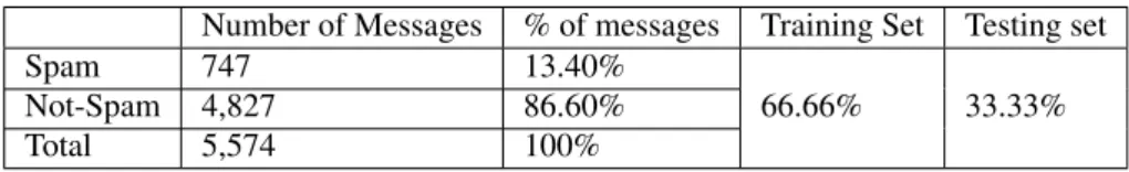
Table 1: Statistics of the dataset
Number of Messages % of messages Training Set Testing set
Spam 747 13.40%
Not-Spam 4,827 86.60% 66.66% 33.33%
Total 5,574 100%
This process was repeated until the loss was deemed to be acceptable. Before the repetition of the new epochs, the weight between the neurons was recomputed based on the loss obtained at the output layer. To minimize chances of model overfitting, a regularization parameter called (dropout) was used with a value between 0-1. The dropout parameter, disables (drops) the connection between the neurons during the training to reduce computational overhead and the likelihood of over-fitting (Kumar & Singh, 2019; Liu et al., 2018).
4. Result Analysis
In this section, we present a comprehensive results of the proposed model. We started our experiment with a machine learning based model in which the features are extracted from the text and then it was given to the classifiers such as: NB (Rish, 2001), RF (Breiman, 2001), GB (Friedman, 2001), LR (Nasrabadi, 2007), SGD (Bottou, 2010). Thereafter, the dataset was fed to the proposed CNN and LSTM model to classify the messages into Spam and Not-Spam class.
For the current research, we have used the benchmark dataset downloaded from the UCI Repository (Almeida et al., 2011). As shown in Table 1, it contains the total number of 5574 instances (Spam and Not-Spam text messages in English). Among them, the Spam messages are 747 and Not-Spam messages are 4827. These messages were collected from a variety of sources. These include Grumbletext–a UK public forum3, the SMS corpus from National University of Singapore, and Caroline Tagg’s PhD Thesis (Tagg, 2009).
4.1. Performance Evaluation
To evaluate the performance of the proposed model, we used the well-known metrics for the classification tech-niques such as, Precision (P), Recall (R), F1-Score (F1), Accuracy and Area Under Receiver Operating Curve (For-man, 2003).
Precision (P): It is defined as the fraction of circumstances in which the correct SMS Spams is returned (Equation 13).
Precision(P)= Tp
Tp+Fp
(13) Recall (R): It is defined as proportion of actual SMS Spams is predicted correctly. Mathematically it is defined in the Equation 14.
Recall(R)= Tp
Tp+Fn
(14)
F1-Score (F1): It is defined as harmonic mean of the precision and recall as given in Equation 15.
F1−S core(F1)=2∗ P∗R
P+R (15)
Accuracy: It is the fraction of SMS Spams Messages that were correctly predicted among the SMS Messages (Equation 16).
Accuracy(A)= Tp+Tn
Tp+Fp+Tn+Fn (16)
We also find the Receiver Operating Characteristic (ROC) curve and find the area under the ROC curve. ROC curve is the plot between True positive rate (TPR) (Equation 17) and False positive rate (FPR) (Equation 18). The area under the ROC curve is used to measure the accuracy of the classifier. Greater the AUC value greater is the accuracy of the model.
T PR= Tp Tp+Fn (17) FPR= Fp Fp+Tn (18) 4.2. Result using the traditional machine learning approach
To classify the text messages into Spam and Not-Spam classes, the extracted textual features are given to the classifiers such as: i) NB, ii) RF, iii) GB, iv) LR, and v) SGD Classifier. The experimentation was started with NB classifier and found that the value of precision (P), recall (R) and F1- Score (F1) for Spam class is 0.21, 0.16 and 0.18 respectively, whereas for Not-Spam class, the values of P, R and F1 is 0.87, 0.90 and 0.89. The obtained result is impressive for the Not-Spam class however for the Spam class the results were very poor. Next the same set of features were given to another traditional machine learning classifier called RF. RF classifier is a ensemble based classifier which work based on the voting mechanism. The RF classifier gives the P, R and F1 values as 0.15, 0.02, and 0.04 for Spam class and 0.86, 0.98 and 0.92 for Not-Spam class. The RF class also yield the better performance for the Not-Spam Class but very poor for Spam class. As the obtained results are not satisfactory, we tested two more classifiers i.e., GB and LR with the same set of features and these classifiers also gave the good results for the Not-Spam only. The detailed results of the selected classifiers are presented in Table 2 and Table 4.
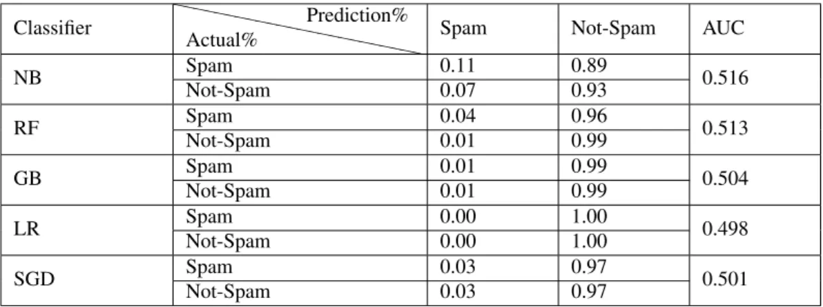
As can be seen from Table 2, all the classifiers give satisfactory results for Not-Spam whereas none of the classifier gave the satisfactory result for Spam prediction. The more detailed result can be seen from Table 3 using the confusion matrix of the classifiers along with the AUC values. These results also confirmed that the set of classifiers are unable to differentiate the Spam and Not-Spam messages efficiently. A probable reason for the poor performance is that the instances of Spam and Not-Spam text messages are not uniformly distributed. The number Spam instances is 747
Table 2: Results using the different classifiers on Imbalanced dataset
Classifier Class Precision (P) Recall (R) F1-Score (F1)
NB Spam 0.213 0.163 0.184 Not-Spam 0.867 0.896 0.883 RF Spam 0.154 0.021 0.036 Not-Spam 0.860 0.980 0.916 GB Spam 0.332 0.018 0.034 Not-Spam 0.871 0.988 0.925 LR Spam 0.000 0.000 0.000 Not-Spam 0.863 0.997 0.925 SGD Spam 0.129 0.022 0.037 Not-Spam 0.862 0.976 0.915
Table 3: Confusion Matrix using the different classifiers on Imbalanced dataset
Classifier ` ` ` ` ` ` ` ` ` ` `` Actual% Prediction%
Spam Not-Spam AUC
NB Spam 0.11 0.89 0.516 Not-Spam 0.07 0.93 RF Spam 0.04 0.96 0.513 Not-Spam 0.01 0.99 GB Spam 0.01 0.99 0.504 Not-Spam 0.01 0.99 LR Spam 0.00 1.00 0.498 Not-Spam 0.00 1.00 SGD Spam 0.03 0.97 0.501 Not-Spam 0.03 0.97
whereas in Not-Spam 4,825 number of data instances are present. To overcome the data imbalance, we balanced the dataset using the SMOTE over sampling technique (Chawla et al., 2002).
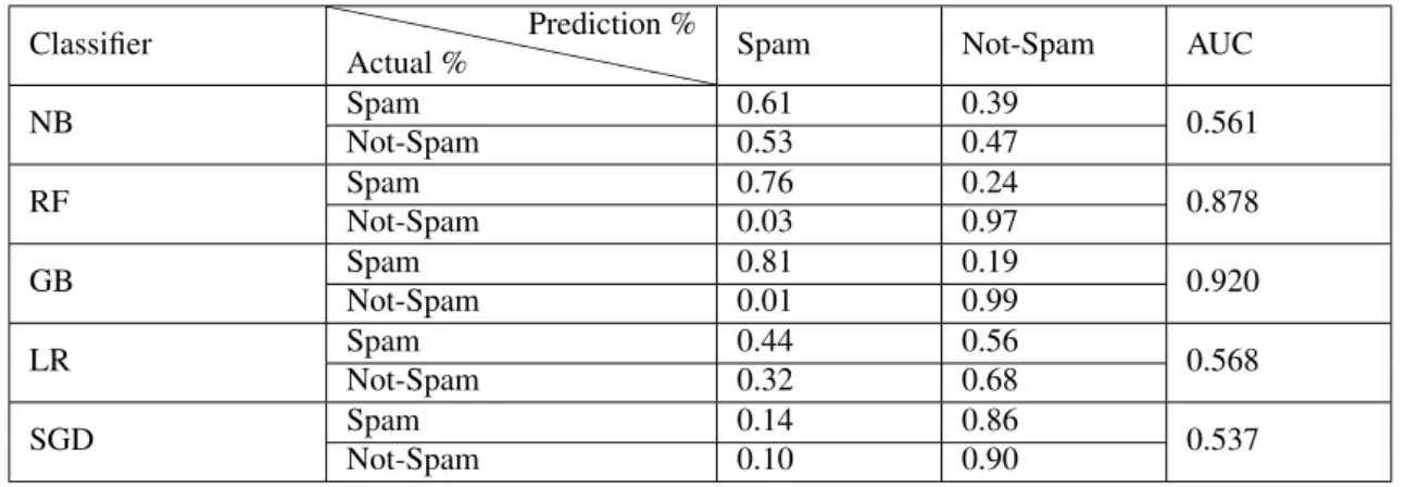
On the balanced version of the dataset, we again applied the same set of classifiers, namely, NB, RF, GB, Logistic Regression, and SGD. The detailed results are presented in Table 4. As can be seen from the Table 4, the results on balanced dataset is improved as compared to unbalanced dataset. The P, R and F1 for the Spam class is 0.99, 0.82 and 0.88 and for Not-Spam class is 0.85, 0.99 and 0.91 respectively using the GB classifier. The obtained results is improved as the recall values is reached to 0.88 for the best case. Recall value 0.88 indicates that 88% of time the Spam message will be predicted as Spam only whereas 12% of time it may be presented as Not-Spam. Since, the SMS messages is directly accessible from the smartphone, it is very important to filter the Spam as much as possible. Since, we checked number of different classifiers and achieved 0.88 recall value which can be improved if a better combination of features set were supplied to the machine learning classifiers. The performance of the traditional machine learning based classifiers can also be seen from the confusion metrics as presented in Table 5.
Table 4: Results on balanced dataset using the different classifiers
Classifier Class Precision (P) Recall (R) F1-Score (F1)
NB Spam 0.549 0.651 0.596 Not-Spam 0.550 0.469 0.506 RF Spam 0.962 0.763 0.851 Not-Spam 0.804 0.971 0.880 GB Spam 0.993 0.809 0.891 Not-Spam 0.839 0.994 0.910 LR Spam 0.581 0.449 0.507 Not-Spam 0.551 0.676 0.607 SGD Spam 0.501 0.753 0.602 Not-Spam 0.504 0.254 0.338
Table 5: Confusion Matrix using the different classifiers on balanced dataset
Classifier ` ` ` ` ` ` ` ` ` ` `` Actual % Prediction %
Spam Not-Spam AUC
NB Spam 0.61 0.39 0.561 Not-Spam 0.53 0.47 RF Spam 0.76 0.24 0.878 Not-Spam 0.03 0.97 GB Spam 0.81 0.19 0.920 Not-Spam 0.01 0.99 LR Spam 0.44 0.56 0.568 Not-Spam 0.32 0.68 SGD Spam 0.14 0.86 0.537 Not-Spam 0.10 0.90
4.3. Result using deep learning approaches
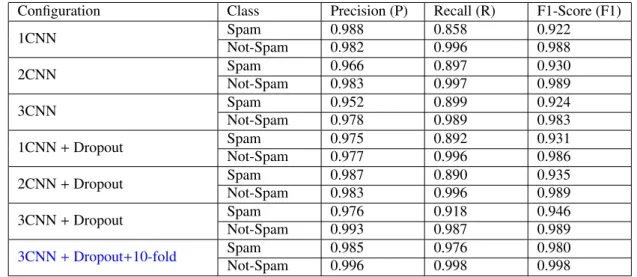
We started with the basic configuration on CNN using a five-gram kernel along with the word vectors created using the Glove (Pennington et al., 2014) model. The batch size was fixed to 30. As can be seen from Table 6, the model yields the P, R, and F1 values as 0.99, 0.86 and 0.92 respectively for Spam prediction. As can be seen from Table 6, the recall value for Spam prediction was not improved, so we tuned the parameters of the model and increase the convolution layer (2CNN) and used three 2-gram, 3-gram, and 4-gram and 5-gram kernels together. With 2CNN, the model yield the P, R, and F1 value as 0.97, 0.90, and 0.93 respectively. The recall value of Spam prediction is increased from 0.86 to 0.90. Further, we increase one more layer of convolution to test whether the performance will increase or not and found the P, R, and F1 value as 0.95, 0.90, and 0.93 respectively with 3CNN. This results confirmed that the 3CNN model does not help to improve the performance of the model, as the recall value of the Spam prediction was same as 2CNN model, but the precision is decreased from 0.97 to 0.95. This experiment confirmed that, adding the convolution layers not help to get more accurate Spam prediction. So, we added the regularization parameter as Dropout on CNN network and test the model with all three configuration i.e., 1CNN, 2CNN, and 3CNN. The detailed results obtained using the different configuration of the CNN models are presented in Table 6 and their confusion matrix is presented in Table 7.
Table 6: The results obtained using the different configurations of CNN models
Configuration Class Precision (P) Recall (R) F1-Score (F1)
1CNN Spam 0.988 0.858 0.922 Not-Spam 0.982 0.996 0.988 2CNN Spam 0.966 0.897 0.930 Not-Spam 0.983 0.997 0.989 3CNN Spam 0.952 0.899 0.924 Not-Spam 0.978 0.989 0.983 1CNN+Dropout Spam 0.975 0.892 0.931 Not-Spam 0.977 0.996 0.986 2CNN+Dropout Spam 0.987 0.890 0.935 Not-Spam 0.983 0.996 0.989 3CNN+Dropout Spam 0.976 0.918 0.946 Not-Spam 0.993 0.987 0.989 3CNN+Dropout+10-fold Spam 0.985 0.976 0.980 Not-Spam 0.996 0.998 0.998
The experimented results confirmed that adding a regularization parameter to the CNN model helps to get more accurate predictions. The best results obtained using the 3-CNN (with dropout) where the P, R and F1 values are 0.98, 0.92 and 0.95 respectively for Spam class prediction whereas for Not-Spam, the model gave the P, R and F1 values as 0.99, 0.99, 0.99 respectively. For the best case, our proposed 3CNN with Dropout and 3CNN with 10-fold cross validation models yielded an accuracy of 98.63% and 99.44% respectively.
We checked another deep learning based model called Long Short-term Memory (LSTM) network in order to improve the recall value of the target class (i.e., Spam) prediction. The detailed results obtained using the LSTM models are presented in Table 8.
As can be seen from Table 6 and Table 8, the results obtained using the CNN and LSTM models were better as compared to the traditional machine earning based classifiers on both the unbalanced dataset (Table 3) and the balanced dataset (Table 5). Also, the experimental results confirmed that among all the experimented variant of machine learning and deep learning algorithms, the deep learning model (3-CNN with Dropout) predicted the Spam and Not-Spam messages correctly with an accuracy of 98.63% on the mentioned size of test sample. The same model when tested with 10 fold cross-validation, where the folds were created through random partitioning, yielded an accuracy of 99.44% as shown in Table 9.
5. Discussion
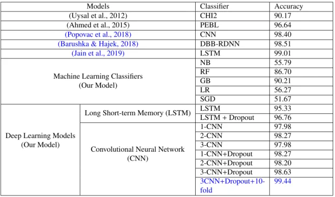
In this paper, a deep learning based model was proposed to filter SMS Spam. The model classified Spam and Not-Spam text messages with a remarkable accuracy of 99.44%. Initially, traditional machine learning-based classifiers were also tested with selected textual feature set. The classification recorded an accuracy of 51.67% with SGD, 55.79% with NB, 56.27% with LR, 86.70% with RF, and 90.21% with GB as shown in Table 9. Later, we tested two different models of deep learning i) CNN and ii) LSTM. The experimental results confirmed that the CNN model
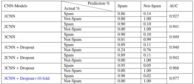
Table 7: The Confusion Matrix of the CNN models CNN-Models ` ` ` ` ` ` ` ` ` ` ` ` Actual % Prediction %
Spam Not-Spam AUC
1CNN Spam 0.86 0.14 0.927 Not-Spam 0.00 1.00 2CNN Spam 0.90 0.10 0.941 Not-Spam 0.00 1.00 3CNN Spam 0.90 0.10 0.949 Not-Spam 0.01 0.99 1CNN+Dropout Spam 0.89 0.11 0.940 Not-Spam 0.24 0.76 2CNN+Dropout Spam 0.89 0.11 0.942 Not-Spam 0.00 1.00 3CNN+Dropout Spam 0.95 0.05 0.968 Not-Spam 0.00 1.00 3CNN+Dropout+10-fold Spam 0.98 0.02 0.977 Not-Spam 0.00 1.00
Table 8: The results obtained using the different configurations of LSTM model
Configuration Class Precision (P) Recall (R) F1-Score (F1)
LSTM Spam 0.849 0.777 0.811 Not-Spam 0.972 0.976 0.973 LSTM+Dropout(0.2) Spam 0.889 0.852 0.870 Not-Spam 0.982 0.976 0.978 LSTM+Dropout(0.3) Spam 0.896 0.842 0.868 Not-Spam 0.977 0.989 0.982
outperformed the LSTM model. We compared the accuracy of the CNN model with the earlier models proposed by (Uysal et al., 2012) and (Ahmed et al., 2015) and found that our model outperformed in terms of classification accuracy as shown in Table 9.We also compared our work with some recent works proposed by (Barushka & Hajek, 2018; Jain et al., 2019; Popovac et al., 2018). Popovac et al. (2018) also used a Convolutional neural network based architecture and achieved an accuracy of 98.4% for the best case. A model called DBB-RDNN-Rel proposed by (Barushka & Hajek, 2018) which achieved 98.51% accuracy for Spam prediction. Jain et al. (2019)used LSTM network (a variant of recurrent neural network) and achieved an accuracy of 99.01%. They used three different word embedding techniques: i) Word2Vec, ii) WordNet, and iii) ConcepNet to achieve the said accuracy. The outcome of our proposed 3CNN with Dropout and 3CNN with 10-fold cross validation models yielded an accuracy of 98.63% and 99.44% respectively.
The paper is significant for both theory and practice. Theoretically, it contributes to the machine learning literature by showing the possibility to mitigate the dependency of feature selection in order to predict SMS Spam and Not-Spam messages. Machine learning-based classification models cannot process textual data. Hence, they need to be provided with a set of relevant features. However, finding the relevant features for any problem is itself a separate research area as it requires the specific domain expertise. In contrast, the proposed deep learning based model such
Table 9: Summary of the experimental results with different models
Models Classifier Accuracy
(Uysal et al., 2012) CHI2 90.17
(Ahmed et al., 2015) PEBL 96.64
(Popovac et al., 2018) CNN 98.40
(Barushka & Hajek, 2018) DBB-RDNN 98.51
(Jain et al., 2019) LSTM 99.01
Machine Learning Classifiers (Our Model) NB 55.79 RF 86.70 GB 90.21 LR 56.27 SGD 51.67
Deep Learning Models (Our Model)
Long Short-term Memory (LSTM) LSTM 95.33
LSTM+Dropout 96.76
Convolutional Neural Network (CNN) 1-CNN 97.98 2-CNN 98.27 3-CNN 97.98 1-CNN+Dropout 98.27 2-CNN+Dropout 98.20 3-CNN+Dropout 98.63 3CNN+Dropout+10-fold 99.44
as CNN and LSTM uses a number of hidden layers to extract the context-dependent features from the text with the help of multiple iterations. Hence, these models do not have such feature dependency. As a result, the proposed CNN based model reduced the major overhead of feature engineering. Also, the model can easily be applied to address any text classification problems such as Email Spam, Web Spam, Blog Spam, and Opinion Spam.
On the practical front, the model developed in this paper could be utilized to filter SMS Spam. There are multiple industry sectors that use SMS to communicate with their customers. These range from banking and e-commerce to travel and insurance as well as online booking portals. It is important to separate legitimate text messages from those that are fraudulent. This will ensure that appropriate text messages from businesses will get the required attention from users while those that are spam are automatically flagged.
6. Conclusion
This paper focused on how to filter SMS Spam efficiently. In particular, it used deep learning based models such as CNN and LSTM along with machine learning based classifiers such as NB, RF, GB, LR, and SGD classifier are tested. The experimental results confirmed that the CNN based model with the regularization parameter (dropout)on
randomly sampled 10-fold cross validation data performed best by securing an accuracy of 99.44%to filter Spam and
Not-Spam text messages. A limitation of the work is that it was dependent on text messages written in English only. Therefore, this paper invites future research to employ similar deep learning approaches to filter Spam and Not-Spam text messages written in other languages too. The efficacy of a similar approach could also be tested on other contexts
of spam such as authentic versus fake online reviews, and real versus fake news.
References
Abdullahi, M., Ngadi, M. A. et al. (2016). Symbiotic organism search optimization based task scheduling in cloud computing environment.Future Generation Computer Systems,56, 640–650.
Ahmed, I., Ali, R., Guan, D., Lee, Y.-K., Lee, S., & Chung, T. (2015). Semi-supervised learning using frequent itemset and ensemble learning for sms classification.Expert Systems with Applications,42, 1065–1073.
AlaM, A.-Z., Faris, H., Hassonah, M. A. et al. (2018). Evolving support vector machines using whale optimization algorithm for spam profiles detection on online social networks in different lingual contexts.Knowledge-Based Systems,153, 91–104.
Almeida, T. A., Hidalgo, J. M. G., & Yamakami, A. (2011). Contributions to the study of sms spam filtering: new collection and results. In
Proceedings of the 11th ACM symposium on Document engineering(pp. 259–262). ACM.
Androulidakis, I., Vlachos, V., & Papanikolaou, A. (2013). Fimess: filtering mobile external sms spam. InProceedings of the 6th Balkan Conference in Informatics(pp. 221–227). ACM.
Androutsopoulos, I., Koutsias, J., Chandrinos, K., Paliouras, G., & Spyropoulos, C. (2000). An evaluation of naive bayesian anti-spam filtering. In
Proceedings of the Workshop on Machine Learning in the New Information Age, 11 th European Conference on Machine Learning(pp. 9–17). Barushka, A., & Hajek, P. (2018). Spam filtering using integrated distribution-based balancing approach and regularized deep neural networks.
Applied Intelligence, (pp. 1–19).
Bengio, Y., Ducharme, R., Vincent, P., & Jauvin, C. (2003). A neural probabilistic language model. Journal of machine learning research,3, 1137–1155.
Bottou, L. (2010). Large-scale machine learning with stochastic gradient descent. InProceedings of COMPSTAT’2010(pp. 177–186). Springer. Breiman, L. (2001). Random forests.Machine learning,45, 5–32.
Chan, P. P., Yang, C., Yeung, D. S., & Ng, W. W. (2015). Spam filtering for short messages in adversarial environment. Neurocomputing,155, 167–176.
Chawla, N. V., Bowyer, K. W., Hall, L. O., & Kegelmeyer, W. P. (2002). Smote: synthetic minority over-sampling technique.Journal of artificial intelligence research,16, 321–357.
Chen, C., Wen, S., Zhang, J., Xiang, Y., Oliver, J., Alelaiwi, A., & Hassan, M. M. (2017). Investigating the deceptive information in twitter spam.
Future Generation Computer Systems,72, 319–326.
Chen, L., Yan, Z., Zhang, W., & Kantola, R. (2015). Trusms: a trustworthy sms spam control system based on trust management.Future Generation Computer Systems,49, 77–93.
Chen, Z., Yan, Q., Han, H., Wang, S., Peng, L., Wang, L., & Yang, B. (2018). Machine learning based mobile malware detection using highly imbalanced network traffic.Information Sciences,433, 346–364.
Cohen, Y., Gordon, D., & Hendler, D. (2018). Early detection of spamming accounts in large-scale service provider networks.Knowledge-Based Systems,142, 241–255.
Dahl, G. E., Yu, D., Deng, L., & Acero, A. (2012). Context-dependent pre-trained deep neural networks for large-vocabulary speech recognition.
IEEE Transactions on audio, speech, and language processing,20, 30–42.
Delany, S. J., Buckley, M., & Greene, D. (2012). Sms spam filtering: methods and data.Expert Systems with Applications,39, 9899–9908. Drucker, H., Wu, D., & Vapnik, V. N. (1999). Support vector machines for spam categorization. IEEE Transactions on Neural networks,10,
1048–1054.
El-Alfy, E.-S. M., & AlHasan, A. A. (2016). Spam filtering framework for multimodal mobile communication based on dendritic cell algorithm.
Future Generation Computer Systems,64, 98–107.
Faulkner, G. (1997). A new and nasty way to flood networks with spam.Computers&Security,7, 622–623.
Fischer, T., & Krauss, C. (2018). Deep learning with long short-term memory networks for financial market predictions. European Journal of Operational Research,270, 654–669.
Forman, G. (2003). An extensive empirical study of feature selection metrics for text classification. Journal of machine learning research,3, 1289–1305.
Friedman, J. H. (2001). Greedy function approximation: a gradient boosting machine.Annals of statistics, (pp. 1189–1232).
Fu, J., Lin, P., & Lee, S. (2014). Detecting spamming activities in a campus network using incremental learning.Journal of Network and Computer Applications,43, 56–65.
Fu, Q., Feng, B., Guo, D., & Li, Q. (2018). Combating the evolving spammers in online social networks.Computers&Security,72, 60–73. Glorot, X., Bordes, A., & Bengio, Y. (2011). Deep sparse rectifier neural networks. InProceedings of the fourteenth international conference on
artificial intelligence and statistics(pp. 315–323).
Goodfellow, I. J., Warde-Farley, D., Mirza, M., Courville, A., & Bengio, Y. (2013). Maxout networks.arXiv preprint arXiv:1302.4389, . Gu, J., Wang, Z., Kuen, J., Ma, L., Shahroudy, A., Shuai, B., Liu, T., Wang, X., Wang, G., Cai, J. et al. (2018). Recent advances in convolutional
neural networks.Pattern Recognition,77, 354–377.
Gupta, V., Mehta, A., Goel, A., Dixit, U., & Pandey, A. C. (2019). Spam detection using ensemble learning. InHarmony Search and Nature Inspired Optimization Algorithms(pp. 661–668). Springer.
Hall, M., Frank, E., Holmes, G., Pfahringer, B., Reutemann, P., & Witten, I. H. (2009). The weka data mining software: an update.ACM SIGKDD explorations newsletter,11, 10–18.
Hancock, B. (2001). Fighting spam in europe.Computers&Security,20, 18–18.
Hinde, S. (2002). Spam, scams, chains, hoaxes and other junk mail.Computers and Security,21, 592–606. Hochreiter, S., & Schmidhuber, J. (1997). Long short-term memory.Neural computation,9, 1735–1780.
Jain, G., Sharma, M., & Agarwal, B. (2019). Optimizing semantic lstm for spam detection.International Journal of Information Technology,11, 239–250.
Jeong, S., Noh, G., Oh, H., & Kim, C.-k. (2016). Follow spam detection based on cascaded social information.Information Sciences,369, 481–499. Jiang, K., Feng, S., Song, Q., Calix, R. A., Gupta, M., & Bernard, G. R. (2018). Identifying tweets of personal health experience through word
embedding and lstm neural network.BMC bioinformatics,19, 210.
Jiang, M., Cui, P., & Faloutsos, C. (2016). Suspicious behavior detection: Current trends and future directions. IEEE Intelligent Systems,31, 31–39.
Jindal, N., & Liu, B. (2007). Review spam detection. InProceedings of the 16th international conference on World Wide Web(pp. 1189–1190). ACM.
Kalchbrenner, N., Grefenstette, E., & Blunsom, P. (2014). A convolutional neural network for modelling sentences.arXiv preprint arXiv:1404.2188, .
Kim, S.-E., Jo, J.-T., & Choi, S.-H. (2015). Sms spam filterinig using keyword frequency ratio.SERSC: International Journal of Security and Its Applications,9, 329–336.
Krizhevsky, A., Sutskever, I., & Hinton, G. E. (2012). Imagenet classification with deep convolutional neural networks. InAdvances in neural information processing systems(pp. 1097–1105).
Kumar, A., & Singh, J. P. (2019). Location reference identification from tweets during emergencies: A deep learning approach. International journal of disaster risk reduction,33, 365–375.
Lai, C.-C. (2007). An empirical study of three machine learning methods for spam filtering.Knowledge-Based Systems,20, 249–254.
Lee, J. Y., & Dernoncourt, F. (2016). Sequential short-text classification with recurrent and convolutional neural networks. arXiv preprint arXiv:1603.03827, .
Lee, K., Caverlee, J., & Webb, S. (2010). Uncovering social spammers: social honeypots+machine learning. In Proceedings of the 33rd international ACM SIGIR conference on Research and development in information retrieval(pp. 435–442). ACM.
Li, L., Qin, B., Ren, W., & Liu, T. (2017). Document representation and feature combination for deceptive spam review detection.Neurocomputing,
254, 33–41.
Transactions on Intelligent Systems and Technology (TIST),10, 6.
Liu, S., Wang, Y., Zhang, J., Chen, C., & Xiang, Y. (2017). Addressing the class imbalance problem in twitter spam detection using ensemble learning.Computers&Security,69, 35–49.
Makkar, A., & Kumar, N. (2019). Cognitive spammer: a framework for pagerank analysis with split by over-sampling and train by under-fitting.
Future Generation Computer Systems,90, 381–404.
Mathew, K., & Issac, B. (2011). Intelligent spam classification for mobile text message. InComputer Science and Network Technology (ICCSNT), 2011 International Conference on(pp. 101–105). IEEE volume 1.
Nasrabadi, N. M. (2007). Pattern recognition and machine learning.Journal of electronic imaging,16, 049901.
Nguyen, D. T., Al Mannai, K. A., Joty, S., Sajjad, H., Imran, M., & Mitra, P. (2017). Robust classification of crisis-related data on social networks using convolutional neural networks. InEleventh International AAAI Conference on Web and Social Media.
Osho, O., Ogunleke, O. Y., & Falaye, A. A. (2014). Frameworks for mitigating identity theft and spamming through bulk messaging. InIEEE 6th International Conference on Adaptive Science and Technology, Ota, Nigeria.
Palaz, D., Magimai-Doss, M., & Collobert, R. (2019). End-to-end acoustic modeling using convolutional neural networks for hmm-based automatic speech recognition.Speech Communication,108, 15–32.
Pascanu, R., Gulcehre, C., Cho, K., & Bengio, Y. (2013). How to construct deep recurrent neural networks.arXiv preprint arXiv:1312.6026, . Pennington, J., Socher, R., & Manning, C. (2014). Glove: Global vectors for word representation. InProceedings of the 2014 conference on
empirical methods in natural language processing (EMNLP)(pp. 1532–1543).
Popovac, M., Karanovic, M., Sladojevic, S., Arsenovic, M., & Anderla, A. (2018). Convolutional neural network based sms spam detection. In
2018 26th Telecommunications Forum (TELFOR)(pp. 1–4). IEEE.
Radford, A., Metz, L., & Chintala, S. (2015). Unsupervised representation learning with deep convolutional generative adversarial networks.arXiv preprint arXiv:1511.06434, .
Rafique, M. Z., Alrayes, N., & Khan, M. K. (2011). Application of evolutionary algorithms in detecting sms spam at access layer. InProceedings of the 13th annual conference on Genetic and evolutionary computation(pp. 1787–1794). ACM.
Rish, I. (2001). An empirical study of the naive bayes classifier. InIJCAI 2001 workshop on empirical methods in artificial intelligence(pp. 41–46). IBM volume 3.
Saumya, S., Singh, J. P., & Dwivedi, Y. K. (2019). Predicting the helpfulness score of online reviews using convolutional neural network. Soft Computing, (pp. 1–17).
Shang, E.-X., & Zhang, H.-G. (2016). Image spam classification based on convolutional neural network. In2016 International Conference on Machine Learning and Cybernetics (ICMLC)(pp. 398–403). IEEE volume 1.
SMS, C. (2018). The real value of sms to businesses.https://www.smscomparison.co.uk/sms-gateway-uk/2018-statistics/, Accesed on March 2019, . Tagg, C. (2009).A corpus linguistics study of SMS text messaging. Ph.D. thesis University of Birmingham.
Uysal, A. K., Gunal, S., Ergin, S., & Gunal, E. S. (2012). A novel framework for sms spam filtering. InInnovations in Intelligent Systems and Applications (INISTA), 2012 International Symposium on(pp. 1–4). IEEE.
Uysal, A. K., Gunal, S., Ergin, S., & Gunal, E. S. (2013). The impact of feature extraction and selection on sms spam filtering. Elektronika ir Elektrotechnika,19, 67–73.
Vorakulpipat, C., Visoottiviseth, V., & Siwamogsatham, S. (2012). Polite sender: A resource-saving spam email countermeasure based on sender responsibilities and recipient justifications.Computers&Security,31, 286–298.
Wan, L., Zeiler, M., Zhang, S., Le Cun, Y., & Fergus, R. (2013). Regularization of neural networks using dropconnect. InInternational Conference on Machine Learning(pp. 1058–1066).
Wang, C., Zhang, Y., Chen, X., Liu, Z., Shi, L., Chen, G., Qiu, F., Ying, C., & Lu, W. (2010). A behavior-based sms antispam system.IBM Journal of Research and Development,54, 3–1.
Wang, C.-C., & Chen, S.-Y. (2007). Using header session messages to anti-spamming.Computers&Security,26, 381–390.
Xia, W., Zhu, W., Liao, B., Chen, M., Cai, L., & Huang, L. (2018). Novel architecture for long short-term memory used in question classification.
Neurocomputing,299, 20–31.
Yamakami, T. (2003). Impact from mobile spam mail on mobile internet services. InInternational Symposium on Parallel and Distributed Processing and Applications(pp. 179–184). Springer.
Yin, W., Sch¨utze, H., Xiang, B., & Zhou, B. (2016). Abcnn: Attention-based convolutional neural network for modeling sentence pairs. Transac-tions of the Association for Computational Linguistics,4, 259–272.
Zainal, K., Sulaiman, N., & Jali, M. (2015). An analysis of various algorithms for text spam classification and clustering using rapidminer and weka.International Journal of Computer Science and Information Security,13, 66.
Zhang, Y.-D., Dong, Z., Chen, X., Jia, W., Du, S., Muhammad, K., & Wang, S.-H. (2019). Image based fruit category classification by 13-layer deep convolutional neural network and data augmentation.Multimedia Tools and Applications,78, 3613–3632.