GLOBAL JOURNAL OF ADVANCED ENGINEERING TECHNOLOGIES AND SCIENCES COMPARISON OF MAXIMUM POWER POINT TRACKING ALGORITHMS FOR PV SYSTEM USING MATLAB/SIMULINK Ch Nayak Bhukya *1 , Abera Eshetu 2& Kalidas Gera3

(1)

[Bhukya

et al.

, 4(11): November, 2017]

ISSN 2349-0292

Impact Factor 2.675

GLOBAL JOURNAL OF ADVANCED ENGINEERING TECHNOLOGIES AND

SCIENCES

COMPARISON OF MAXIMUM POWER POINT TRACKING ALGORITHMS FOR

PV SYSTEM USING MATLAB/SIMULINK

Ch Nayak Bhukya

*1

_{, Abera Eshetu}

2

_{& Kalidas Gera}

3

*1,2&3

_{Dept. of Electrical and Computer Engineering, Assosa University, Assoa, Ethiopia}

ABSTRACT

Maximum power point tracking (MPPT) is animportant part of solar photovoltaic (PV) system. It increases the efficiency of a solar panel by tracking the maximum power point. There are several MPPT control algorithms in use. In this paper, four control algorithms are analyzed comparatively [1]. Using MATLAB/Simulink a solar PV system with MPPT controlled buck-boost dc-dc converter is modeled. Then the efficiency of each algorithm is calculated using typical daily insulation and temperature variation. Finally, a comparative analysis of the algorithms is presented.

KEYWORDS: Solar photovoltaic; Maximum power point tracking; P&O ; Incremental Conductance; Fuzzy logic; Simulink..

INTRODUCTION

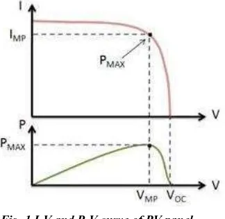
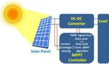
When a PV panel is directly connected to a load, the operating point is rarely at maximum power point. The maximum power point tracker maintains the PV array operating point at maximum power point. Fig. 1 shows the I-V and P-V characteristic curve and maximum power point of a PV panel. To track the maximum power point a dc-dc converter is placed between the panel and the load. The converter’s duty cycle is set such that the power flow from the panel is maximum and the load voltage is as per requirement. The I-V characteristic of solar panel depends on the irradiance and cell temperature. So, the maximum power point changes with varying conditions and the duty cycle also needs to be changed accordingly. The tracker uses some control algorithm to do this task. Fig. 2 shows a block diagram of solar PV system with MPPT.

Fig. 1 I-V and P-V curve of PV panel.

(2)

[Bhukya

et al.

, 4(11): November, 2017]

ISSN 2349-0292

Impact Factor 2.675

open-circuit voltage and fractional short-circuit current algorithms are relatively easier and cheaper to implement. In recent time, some artificial intelligence based algorithms have emerged such as fuzzy logic based algorithm, stimulated annealing, particle swarm optimization etc. In this paper, four algorithms are analyzed namely perturb-and-observation, incremental conductance, fractional open-circuit voltage and fuzzy logic based method. The efficiency of the algorithms is determined from (1).

 

1

0 0



 _t

MAX t

actual mppt

dt t P



Where is the actual (measured) power produced by the PV array under the control of the MPPT, and is the true maximum power the array could produce under a given temperature and irradiance.

Fig. 2 Block diagram of solar PV system with MPPT.

DESCRIPTION OF ANALYSED MPPT ALGORITHMS

A. Perturb and observe (P&O)

The Perturb and observe algorithm is the most commonly

used in practice because of its ease of implementation. In the P&O algorithm, the operating voltage of the PV array is perturbed by a small increment, and the resulting change in power, P, is measured. If P is positive, then the perturbation of the operating voltage moved the PV array’s operating point closer to the MPP. Thus, further voltage perturbations in the same direction (that is, with the same algebraic sign) should move the operating point toward the MPP. If P is negative, the system operating point has moved away from the MPP, and the algebraic sign of the perturbation should be reversed to move back toward the MPP. These can be summarized using the Table I [3].

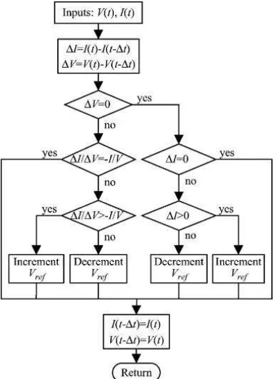
B. Incremental Conductance (IC)

The incremental conductance method is based on the fact that the slope of the PV array power curve is zero at the MPP, positive on the left of the MPP, and negative on the right, as seen in the Fig. 2 [3].

TABLE I.

SUMMARY OF P&O ALGORITHM

Perturbatio n

Change in Power

Next

perturbation

Positive Positive Positive

Positive Negative Negative

Negative Positive Negative

(3)

[Bhukya

et al.

, 4(11): November, 2017]

ISSN 2349-0292

Impact Factor 2.675

dP /dV =0, at MPP,

dP /dV >0, left of MPP,

dP /dV <0, right of MPP.

Since,

 

_{ }

₂

V V V I dV dI V I dV

IV d dV dP

      

∆I/ΔV = -I/V, at MPP.

∆I/ΔV > -I/V, left of MPP.

∆I/ΔV < -I/V, right of MPP.

Fig. 3 Flow chart of Incremental Conductance algorithm.

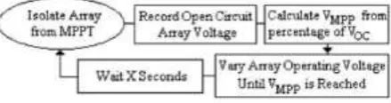
C. Fractional Open Circuit Voltage

(4)

[Bhukya

et al.

, 4(11): November, 2017]

ISSN 2349-0292

Impact Factor 2.675

The constant voltage algorithm can be implemented using the flowchart shown in Fig. 4. The solar array is temporarily isolated from the MPPT, and a measurement is taken. Next, the MPPT calculates the correct operating point using Equation and the pre set value of K, and adjusts the array’s voltage until the calculated is reached. This operation is repeated periodically to track the position of the MPP [2].

Although this method is extremely simple, it is difficult to choose the optimal value of the constant K. The literature reports success with K values ranging from .71 to .80. In this paper, K=.71 was used as it gives the best efficiency.

Fig. 4 Flowchart of fractional open circuit voltage algorithm.

D. Fuzzy Logic based algorithm

Recently fuzzy logic controllers have been widely used for industrial processes owing to their simplicity and effectiveness for both linear and nonlinear systems. A MPP search based on fuzzy logic does not need any parameter information. It consists of a step wise adaptive search as well as leads to fast convergence. The fuzzy controller consists of three functional blocks: 1) Fuzzification, 2) Fuzzy rule algorithm and 3) Defuzzification [5]. Also the fuzzy logic controller should be modified and optimized base on the system it is controlling. In this thesis, we devised a fuzzy logic controlled MPPT which is optimized for this MPPT system.

These functions are described as follows:

1) Fuzzification: The fuzzy logic based MPPT method hastwo input variables, namely dP(k) and dV(k), at a sampling instant k. The output variable is dD(k+1) which is duty cycle change that causes voltage to change at next sampling instant

(k+1). The variable dP(k) and dV(k) are expressed as follows:

dP(k)=P(k)-P(k-1) (4)

dV(k)=V(k)-V(k-1) (5)

In Fig. 5(a), the membership functions of the input variable dP(k) is assigned five fuzzy sets, including positive big (PB), positive small (PS), zero (ZE), negative small (NS), and negative big (NB). The membership functions are denser at the center in order to provide more sensitivity against variation in the PV array terminal voltage. In Fig. 5(b), the membership functions of the input variable dV(k) is assigned three fuzzy sets, including positive (P), zero (Z), and negative(N). Fig. 5(c) shows the membership functions of the output variable dD(k+1) which is assigned fuzzy sets, including positive big (PB), positive middle (PM), zero (ZE), negative middle (NM), and negative big (NB).

(5)

[Bhukya

et al.

, 4(11): November, 2017]

ISSN 2349-0292

Impact Factor 2.675

(a)

(b)

(c)

Fig. 5 Membership function of (a) dP(k), (b) dV(k) and (c) dD(k+1)

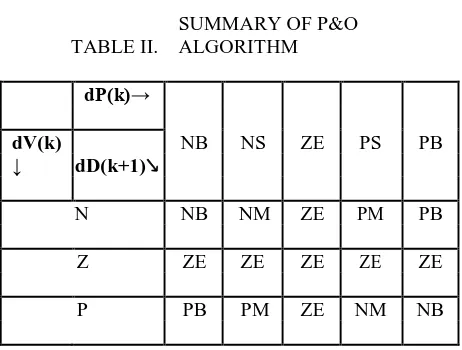
TABLE II.

SUMMARY OF P&O ALGORITHM

dP(k)→

NB NS ZE PS PB dV(k)

↓ dD(k+1)↘

N NB NM ZE PM PB

Z ZE ZE ZE ZE ZE

P PB PM ZE NM NB

3) Defuzzification: After the rules have been evaluated, thelast step to complete the fuzzy control algorithm is to calculate the crisp output of the fuzzy control with the process of defuzzification. The well known center of gravity method for defuzzification is used here. It computes the center of gravity from the final fuzzy space, and yields a result which is highly related to all of the elements in the same fuzzy set. The crisp value of control output dD(k+1) is computed by the following equation:

 

6

1 1

    

n

i i W n

i i dD i W

dD

(6)

[Bhukya

et al.

, 4(11): November, 2017]

ISSN 2349-0292

Impact Factor 2.675

D(k+1) = D(k) + dD(k+1) (7)

Approaches infinity the terminal equation for the current and voltage of the array becomes as follows.

Using the steps mentioned above, the fuzzy controller was implemented in real time for MPPT.

MODELING OF SOLAR PV SYSTEM WITH MPPT

To analyze the efficiency of the MPPT algorithms a solar PV system with MPPT is modeled in MATLAB/Simulink. First Solar PV panel, DC-DC converter with battery and MPPT block were modeled and then they were connected to make the system.

A. PV panel modeling

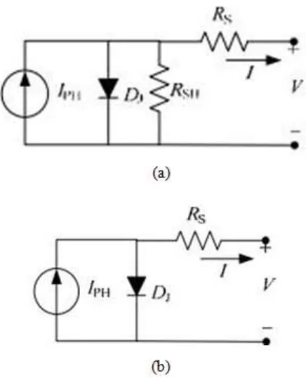
A general mathematical description of I-V output characteristics for a PV cell has been studied for over the past four decades. Such an equivalent circuit-based model is mainly used for the MPPT technologies [4]. The equivalent circuit of the general model which consists of a photo current, a diode, a parallel resistor expressing a leakage current, and a series resistor describing an internal resistance to the current flow, is shown in Fig. 6. The

voltage-current characteristic equation of a solar cell is given as





_{ }

8 1 exp _                          SH S C S S PH R IR V A KT IR V q I I I

Is the cell saturation of dark current, q (=1.6x10-19 C) is an electron charge, k (=1.38x10-23 J/K) is a Boltzmann’s constant, TC is the cell’s working temperature, A is an ideal factor, RSH is a shunt resistance, and

RS is a series resistance. The photocurrent mainly depends on the solar insolation and cell’s working

temperature, which is described as,







SC I C ref





 

9

PH I K T T

I   

Where is the cell’s short-circuit current at a 25° C and 1kW/ 2_{, is the cell’s short-circuit current temperature}

coefficient, is the cell’s reference temperature, and λ is the solar irradiance in kW/ 2_{. On the other hand, the}

cell’s saturation current varies with the cell temperature, which is described as





 

10

1 1 exp 3                          KA T T qE T T I

I ref C

G ref

C RS S

Where IRSthe cell’s reverse saturation is current at a reference temperature and a solar irradiationEGis the

bang-gap energy of the semiconductor used in the cell. The ideal factor A is dependent on PV technology.

The shunt resistance RSH is inversely related with shunt leakage current to the ground and it can be assumed as

infinity without leakage current to ground. The appropriate model of PV solar cell with suitable complexity is shown in (11). Equation (8) can be rewritten to be





_{ }

11 1 exp                   A KT IR V q I I C S S PH I

Since a typical PV cell produces less than 2W at 0.5V approximately, the cells must be connected in series-parallel configuration on a module to produce enough high power. The equivalent circuit for the solar module arranged inNp parallel and Ns series is shown in Fig. 2(a). As shunt resistance.

(7)

[Bhukya

et al.

, 4(11): November, 2017]

ISSN 2349-0292

Impact Factor 2.675

Fig. 6 (a) General model and (b) appropriate model of a solar cell

Fig. 7 generalized model of a PV array.

Since normally IPH>>IS and ignoring the small diode and ground-leakage currents under zero-terminal voltage,

the short-circuit ISC is approximately equal to the photocurrent. On the other hand, the VOC parameter is obtained

by assuming the output current is zero. Given the PV open-circuit voltage at reference temperature and ignoring the shunt-leakage current, the reverse saturation current at reference temperature can be approximately obtained as,

 

₁

 

13

exp

    

 

    

 

    

  

A NsKT

Voc q

Isc I

(8)

[Bhukya

et al.

, 4(11): November, 2017]

ISSN 2349-0292

Impact Factor 2.675

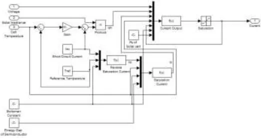
Fig. 8 Solar panel model

Using these equations a generalized solar panel mask model was made in MATLAB/Simulink [3]. The solar panel.

The MPPT block contains necessary parameters and codes for implementing MPPT. Fig. 12 shows subsystemmodel takes voltage, irradiance and cell temperature as input and gives current as output.

Fig. 9 Subsystem implementation of generalized PV array model.

B. DC-DC converter modeling

The buck converter is a step down converter where boost is step up converter. The buck-boost converter can act both as a step up and step down converter according to the duty cycle

[6]. This topology was used for DC-DC converter for MPPT system. In Simulink, SimPowerSystems library was used to create a buck-boost converter. The input was connected to the solar panel block and output with a battery. MOSFET was used as the switch.

(9)

[Bhukya

et al.

, 4(11): November, 2017]

ISSN 2349-0292

Impact Factor 2.675

(b)

Fig. 10 (a) MATLAB model and (b) subsystem implementation of buck-boost converter with battery as load

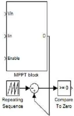
C. MPPT modeling

MPPT block can be described as the brain of the system. It controls the duty cycle of the converter by using some algorithm to track the MPP of the solar panel. After the duty cycle, D is calculated it is converted to pulses using repeating sequence, sum and compare to zero block. The PWM frequency was selected to be 20 KHz. Fig. 11 shows the Simulink model.

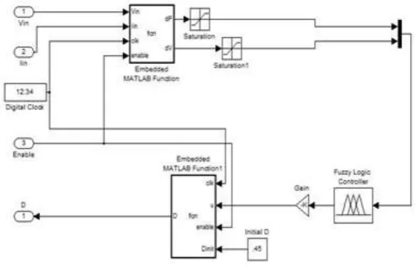
The Embedded MATLAB Function block contains codes. For P&O, IC and fractional open circuit voltage algorithms MATLAB codes were written using Table I, Fig. 3 and Fig. 4. Fuzzy Logic based algorithm subsystem implementation is different from Fig. 12 and presented in Fig. 13

(10)

[Bhukya

et al.

, 4(11): November, 2017]

ISSN 2349-0292

Impact Factor 2.675

Fig. 12 Subsystem implementation of P&O, IC and fractional open circuit voltage MPPT block.

Fig. 13 MATLAB/Simulink based PV array MPPT system.

D. Total PV system modelling

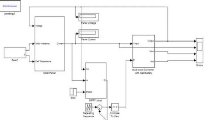
The PV panel block, Converter with battery block and MPPT block previously created were connected as the Fig. 14.

The output of the solar panel block is the panel current (Iinput) and is connected to the input of the converter. The

converterwith battery block gives panel voltage (Vinput), Load voltage (Vout) and current (Iout) as the output.

Panel voltage (Vinput) is input of the solar panel block. The MPPT block takesVinputand Iinputas the input and gives

(11)

[Bhukya

et al.

, 4(11): November, 2017]

ISSN 2349-0292

Impact Factor 2.675

Fig. 14 MATLAB/Simulink based PV array MPPT system.

SIMULATION

The MPPT algorithms were simulated for two profiles of solar irradiance and cell temperature. Case 1 depicts when the irradiance and temperature undergoes relatively low changes. The irradiance level changes from 800 W/m2_{to 1000 W/m}2_{and then to 900 W/m}2_{. The temperature changes from 30°C to 32°C.}

Case 2 depicts the condition when the irradiance andTemperature is highly varying. The irradiance level changes from 600 W/m2_{to 400 W/m}2_{to 500 W/m}2_{to 700 W/m}2_{and finally to 900 W/m}2_{. The temperature}

changes from 26°C to 25°C to 27°C. The time duration for both cases of simulation duration was 1.02 sec and MPPT was enabled after.02 second.

Fig. 15 Irradiance and temperature profile for (a) Case 1 and (b) Case 2

Simulation was done for 5 cases. First case was no MPPT or the battery was directly connected to the panel. The voltage and current were multiplied and then taken to workspace to calculate the harvested energy. Similarly, simulation were done for perturb and observation, incremental conductance, fractional open circuit voltage and fuzzy logic based.

To determine the true maximum power the array could produce under a given temperature and irradiance the P-V curves were plotted under that condition. From that curve the maximum available power were determined.

RESULTS

(12)

(13)

[Bhukya

et al.

, 4(11): November, 2017]

ISSN 2349-0292

Impact Factor 2.675

Fig. 16 Actual maximum power available (blue line) and power produced by PV array with (a) no MPPT, (b) P&O, (c) IC, (d) Fractional open circuit voltage and (e) fuzzy logic based MPPT algorithm (red line)

(14)

[Bhukya

et al.

, 4(11): November, 2017]

ISSN 2349-0292

Impact Factor 2.675

Fig. 17 Average efficiency of Solar PV system with and without different MPPT algorithms

CONCLUSION

Fig. 17 presents a comparison of the efficiencies of four MPPT control algorithms with no MPPT situation. From the simulation results we found that all MPPT algorithms performed much better than the case where no MPPT was used. So, we can say that using MPPT can increase the efficiency of the solar PV system considerably.

The fractional open circuit voltage method was the simplest considering ease of implementation and number of sensors but its performance was least impressive with 93.89% efficiency. Other three MPPT algorithms have higher efficiency. Among them Perturb and observation is the most popular algorithm and by optimizing the step size we found out that its performance is satisfactory with 98.43% efficiency. Incremental Conductance has higher efficiency (98.57%) than P&O and Fuzzy logic based algorithm has the highest efficiency (98.67%). We also found out that among the four algorithms fuzzy logic based algorithm performed best in case 1 and incremental conductance on case 2. On an average basis the fuzzy logic based algorithm outperformed other algorithms. But the complexity of implementing higher implementation cost can only be justified in much larger PV systems.

REFERENCES

[1] Md. Rashed Hassan Bipu, Syed Mohammad Sifat Morshed Chowdhury, Manik Dautta and Md. Zulkar Nain. 2014. Study and analysis of solar charge controller and different mppt algorithms, B.Sc. Thesis, Bangladesh University of Engineering and Technology.

[2] D. P. Hohm and M. E. Ropp, “Comparative Study of Maximum Power Point Tracking Algorithms”, PROGRESS IN PHOTOVOLTAICS: RESEARCH AND APPLICATIONS, Published online 22 November 2002.

[3] Trishan Esram and Patrick L. Chapman, “Comparison of Photovoltaic Array Maximum Power Point Tracking Techniques”, IEEE TRANSACTIONS ON ENERGY CONVERSION, VOL. 22, NO. 2, JUNE 2007.

[4] Huan-Liang Tsai, Ci-Siang Tu, and Yi-Jie Su, “Development of Generalized Photovoltaic Model Using MATLAB/SIMULINK”, Proceedings of the World Congress on Engineering and Computer Science 2008, San Francisco, USA.

[5] Jiyong Li and Honghua Wang, “Maximum Power Point Tracking of Photovoltaic Generation Based on the Fuzzy Control Method”.M. Young, The Technical Writer’s Handbook. Mill Valley, CA: University Science, 1989.