Multi-Stage Meta-Learning for Few-Shot with Lie Group Network Constraint

Multi-Stage Meta-Learning for Few-Shot with Lie

Group Network Constraint

Fang Dong1,, Fanzhang Li1,*

School of Computer Science and Technology, Soochow University, Suzhou 215006, Jiangsu, China; [email protected](F.D.)

* Correspondence: [email protected]

Abstract:Deep learning has achieved lots of successes in many fields, but when trainable sample are extremely limited, deep learning often under or overfitting to few samples. Meta-learning was proposed to solve difficulties in few-shot learning and fast adaptive areas. Meta-learner learns to remember some common knowledge by training on large scale tasks sampled from a certain data distribution to equip generalization when facing unseen new tasks. Due to the limitation of samples, most approaches only use shallow neural network to avoid overfitting and reduce the difficulty of training process, that causes the waste of many extra information when adapting to unseen tasks. Euclidean space-based gradient descent also make meta-learner’s update inaccurate. These issues cause many meta-learning model hard to extract feature from samples and update network parameters. In this paper, we propose a novel method by using multi-stage joint training approach to post the bottleneck during adapting process. To accelerate adapt procedure, we also constraint network to Stiefel manifold, thus meta-learner could perform more stable gradient descent in limited steps. Experiment on mini-ImageNet[1] shows that our method reaches better accuracy under 5-way 1-shot and 5-way 5-shot conditions.

Keywords:meta-learning; lie group; machine learning; deep learning; convolutional neural network

1. Introduction

With the rapid improvement of computer performance and the scale of trainable data, deep learning models trained on large scale dataset could achieve huge improvement, some of them even has better performance than human in many scenes like classification[2] and regression. Most deep learning model could increase performance as the trainable data increase. But not every field has enough data using in training model, tradition deep learning models are difficult to have the same level learning ability and adaptability as humans when number of trainable samples is seriously insufficient.

One of the great advantages of human intelligence is that even children can learn to recognize new unseen things through few information. For example, give child a image of certain animal, and he can use it to grasp the feature of this species, and easily identify them when facing other images of this animal. The logic behind this example is that human beings can complete the construction of new task’ s feature and structures through the existing knowledge, and master faster and more accurate learning methods based on the continuous experience. Tradition deep learning models are dedicated to extracting embedding features from large scale data which belong to the same distribution and use them to classify new samples. Thus, once the trainable data amount is insufficient, or be required to quickly adapt to new unseen tasks, tradition models are difficult to deal with.

Meta-learning is used to explore and handle machine learning problems with limited trainable data. The state-of-the-art approach in this field is Model-Agnostic Meta-Learning[3], which denoted as MAML, this model provides a whole new structure to enhance the generalization performance. Generally, MAML-based models contain three parts: i) common initial basics; ii) adapting process and iii) gradient based updating rules to change network parameters inside meta-learner. These three parts correspond to the basic knowledge, learning process and learning approach in human’s

learning process in order. Meta-learning models usually embed a meta-learner which used to save and generate initial parameters. Meta-learner can adapt to new unseen tasksT by finetuning network parameters from few samples which has same classes inT. After meta-learner adapting to unseen taskT, some new samples are used to measure the performance of meta-learner by accuracy, then model use optimizer to optimize the loss function object to update the whole model.

Since the adapting rule of meta-learner is fixed in MAML and model updates all parameters in meta-learner’s network, MAML needs much more time to converge. Also, MAML starts training meta-learner from a randomly initialized networkθ, this force the model updatesFeature Extractor andClassify Layerof meta-learner at the same time, Arnoldet al.[4] point out that MAML-based models need much more network parameters than theoretically needed, because they should handle basic knowledge and new knowledge in one network, and meta-learner use low-level layers to extract features from sample data, use high-level layers such as full connect linear layer to classify.

As mentioned in Arnold’s conclusion, tiny change in high-level layers contribute much more performance than layers in feature extractor during meta-test phase, so model can hardly optimize feature extractor and classify layer from few samples. Most of meta-learners in MAML-based methods only hold a shallow network which use few convolution layers as feature extractor. This factor further limits the meta-learner’s ability to extract embedding features. In this paper, we tried deeper network structure by perform pretrain on meta-learner’s feature extractorφ. Many excellent methods[5][6][7] in meta-learning area execute pretrain to seek a feature extractor with enough generalization. Pretrained on large scale data could let meta-learner focus more on how to do better classify based on higher utilization of samples.

The updating rule is another issue of MAML that meta-learner perform evaluation on each step in adapting process, but only the last evaluation result been taken into to judge the performance of model. Meta-learner often executes multi updates in adapting process, it’s obviously that test accuracy on new samples increase with the gradient descent performed on meta-learner’s network and the increasement of accuracy is not linear related to steps, the increasement severely reduces in the middle and late stage in adapting process, updating process would easily falls into the bottleneck without manual intervention. Thus, we introduce multi-stage optimization method into MAML-based method. Model sets some checkpoints during the middle and late stage in adapting process to improve performance when stucks. This approach improves the utilization rate of training data under the limited update steps. Differential based gradient descent often applied in adapting process, therefore even if the network is very shallow, it still cannot guarantee the stability and the accuracy of direction in every gradient descent step, especially for the scene that trainable sample and number of update steps are extremely few.

In order to make up for the shortcomings that too much randomness in gradient descent, this paper introduces method which used in Manifold learning that define network under the orthonormal constraints. By constraint network geometry as Stiefel manifold or Lie group, the gradient on this network can be presented by Lie algebra and projection from orthogonal spaceO(m)to Stiefel manifold spaceSt(m,n). This constraint reduces the scale of parameter search space during gradient descent and improve the accuracy of gradient descent. In the remainder of this paper, we discuss detail of methods and then execute experiment on open source image dataset mini-ImageNet to evaluate our method.

The concept of meta-learning has been proposed decades ago, it first appear in education industry[8][9][10] to represent a frame that students should make better use of existing knowledge during learning and acquire better performance by mastering some basic knowledge and cooperating with continuous improvement of learning methods in the life-long learning process.

cosine distance;the second approach use a small extra neural network to replace gradient descent by outputting the corrected gradient value during adapting process[13] to makes meta-learner learn how to learnandwhat to learnrather than just learn a initial value;the third waybased on gradient descent, most of them based on MAML’s framework. These models update every layer of the neural network inside meta-learner by apply gradient descent. Specifically, MAML-based approach is the state-of-the-art algorithm in meta-learning field.

The detail of MAML algorithm is to embed meta-learner, a fully functional neural network model, into meta-learning model. It uses meta-learner to adapt to unseen tasks by learning from training data and output predictions. These methods constitute a dual-layer loop structure, this dual-layer loop allows model optimize the adapting process as a whole to equip initial knowledge with great generalization performance. MAML is also a framework for training and the design a model, thus it has better versatility even in reinforcement learning[14][15][16].

Based on MAML, Probabilistic model-agnostic meta-learning[17] introduces probabilistic into model to represent initial data, Kim[18] and Gupta[19] proposed Bayesian way into MAML to establish relationship between post result and pre data by Bayesian prior probability. Meta-SGD[20] and Task-Agnostic Meta-Learning(TAML)[21] try to make meta-learner learn how to learn better rather than only remember initial knowledge.

After deeper neural networks such as Residual network(ResNet)[22] and Dense network[23] been applied in machine learning, Qiaoet al.[5]’s experiment shows that meta-learner could benefit from deeper and more complex network and model could has much better feature extractor ability, as mentioned by Arnoldet al.[4] above. Training of meta-learner becomes harder with the scale expanded, which not only reflected in program running speed but also the stability during training.

To reduce the amount of parameters need to be updated, Rusuet al.[6] mapping parameters to a low-dimensional latent space as a way to reduce dimensions, then calculate gradients in latent space to make gradient descent more stable. Sunet al.[7] also work on this direction by reducing the number of parameters need to be optimized. We show that the most important part of MAML-based models is feature extractor in experiment. Our meta-test approach comes from Meta-Transfer Learning for Few-Shot Learning(MTL).

The idea that optimize the gradient descent itself by explore the geometry of homogeneous space exists for many years, often treat networks as matrices in Manifold learning[24][25] and Lie group learning[26][27] and constraint matrices to orthogonal group. Nishimoriet al.[28] explore the gradient on high-dimension space and this allows meta-learner make better use of limited data and information in Euclidean space. Nishimori also derived this theory to a more general case which treat linear layer as Stiefel manifold which orthogonal constrainted and use Lie group transitive to simplify calculation process to a linear approximation. Yang et al.[29] has taken this approach in image classification problem and got excellent performance.

2. Methods

Meta-learning model using lots of tasks{T } ∼P(T)to train meta-learner whichT is the smallest cell of training data, also denoted asmeta-task. Training batch contains multi tasks, each task consists of{Ttra,Tqry}. Meta-learner updates network parameters by usingTtra, then got prediction onTqry. The common setup for few-shot learning problem is(5-way 1-shot)and(5-way 5-shot), it means each task consists of 5 classes of data, the count of training samples is 1 or 5, the number of samples used to update model denoted asKshot. The diagram ofT is shown in Figure 1.

For example,(5-way 1-shot)learning problem means meta-learner been used to classify 5 classes with only one trainable sample. A full train-test process contains two parts:meta−trainandmeta−

࣮௧௥௔ ࣮௤௥௬

ǥ

ǥ

ǥ ǥ ǥ ǥ

ݓܽݕ

ܭݍݑ݁ݎݕ ǥ

ǥ

ǥ ǥ ǥ ǥ

ܭݏ݄݋ݐ

Figure 1.Overview of a taskT used in meta-train phase includesTtraandTqry. As described above, the number ofTtraisKshotand the number ofTqryisKquery.

ߠ଴௣௥௘

ߠ଴௣௢௦௧

ߠଵ௣௥௘

ߠଵ௣௢௦௧

ߠ௠௣௥௘

ߠ௠௣௢௦௧ ࣮௧௥௔

ْ

ْ ْ

࣮௤௥௬

ࣦ௤௥௬଴ ࣦ௤௥௬ଵ ࣦ௤௥௬௠

ْ

ْ ْ

ܵݑ݉ሺ _ǥ ሻ

ܥ݄݁ܿ݇݌݋݅݊ݐݏሺ ͳǣ ݓ଴ Ͳǣ ݓଵ Ͳǣ ݓଶ ǥ ͳǣ ݓ௠ሻ

՜ ࣦ

ሺ݂

೘೛೚ೞ೟ሿ

ሻ

ْǣ ݑ݌݀ܽݐ݁ ݋݊ ܵݐ݂݈݅݁݁ ݂݉ܽ݊݅݋݈݀ ߠ଴௣௥௘ǣ ݅݊݅ݐ݈݅ܽ ݊݁ݐݓ݋ݎ݇ ݌ܽݎܽ݉݁ݐ݁ݎݏ ߠଶ௣௥௘

ߠଶ௣௢௦௧ ْ

ْ

ࣦ௤௥௬ଶ

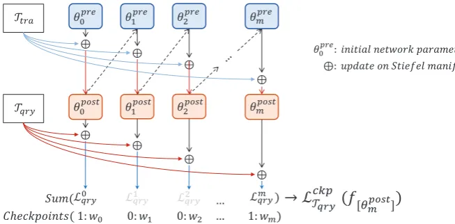
Figure 2.Diagram of our method, a fully inner loop process to optimize networkθin meta-learner.

Meta-task often splitted into two parts:{Ttra,Tqry}, there areKshotsamples inTtraandKqrery samples inTqry. When meta-learner finish learning fromTtra, model generate loss function based on the prediction onTqry, then use optimizers such as SGD or Adam[30] to optimize it.

In this paper, we denote the process which meta-learner update its parameters byTtraasinner loop, and denote the optimizing process on meta-learning model asouter loop. Therefore, we conclude that the largest different between no-meta-learning structure model and MAML-based model is that MAML-based model not only optimize the performance of meta-learner’s prediction accuracy but also make it possible that optimize the process as a whole, no matter what meta-learner did and how it did during inner loop. After every inner loop finished, model got a loss function object, this setup allows model to use almost any approach to optimize the result from inner loop process. The updating rules of inner and outer loop in MAML as follows.

θk,i=θk,i−1−α∇_θk,i−1LT_kf(θk,i−1) (1)

θ←θ−β∇_θ(

∑

k∼BatchLTk(f(θk,m))) (2)

2.1. Pretrained by Large Scale Data

Training of parameters of meta-learner’s network starting from randomly initialization in meta-train phase, it causes that every single parameter in meta-learner requires been updated to fit few-shot setup conditions. The whole model should focus more on how to adapt under a series of limitations rather than learns how to extract features from samples. Recently many meta-learning models split meta-learner into two pieces logically:Feature extractorandClassify layer, thus some models trend to pretrain the feature extractor part on large scale dataset[5][6][7]. Starting meta-train phase after pretrain process completed can greatly reduce the pressure of meta-learner.

Models in few-shot learning and some transfer learning approaches actually learn bias which related to new tasks of their parameters[31]. Our approach of pretrain consists with Sunet al.[5], first construct a model with deep neural network trained on mini-ImageNet dataset’s subset[train∪val], then save weights except classify layer. Additionally, we transfer these parametersφto another model to classify dataset’s test set and only update last classify layer to confirm the performance of this feature extractor. updating rule shows in equation (3).

θ←θ−α∇_{θf c}Lf(θ) (3)

We draw conclusion that it’s possible to extract features from other data with different classes using network trained on large scale dataset. The pretrain algorithm is summarized in Algorithm 1.

Algorithm 1Pretrain

Require: D:{batch} ∼p(T)on large dataset

Require: α,epoch: learning rate and number of training epoches

1: Randomly initialize feature extractorφand classify layerθ

2: DenoteLas loss function 3: fori<epochdo

4: whilenot donedo

5: Sample mini-batch{(x0,y0),(x1,y1)..}fromD

6: Optimize [φ,θ] by gradient descent:φ←φ−α∇φLmini−batch(f[φ,θ]),

θ←θ−α∇_θLmini−batch(f[φ,θ]) 7: end while

8: end for

9: Save parametersφas pretrain initialφpre

Training feature extractor on different dataset could reduce the burden of meta-learner during adapting processes and improve the whole model performance significantly. We modify updating methods both in inner loop and outer loop, for inner loop part, meta-learner only apply gradient descent on its classify layer and fix other parameters, this can speed up program speed and reduce space cost; for outer loop, still not every parameter get optimized, model optimizes meta-learner’s classify layer, all bias, convolutions layers which its filter’s kernel size is(1×1)and related batch normalization parameters. Specifically, our meta-learner uses wide residual network[32] with deep scaleWRN-Kfor 10, selective optimization reduce the number of parameters need to be updated by 90.9% compared to method of MTL[7]. Our optimize principle trends to updating inductive biases of network to keep the ability of continuous adapting.

2.2. Multi-Stage Optimization

test the performance at regular intervals to identify problems and make improvements on a timely basis rather than only focus on last exam result.

Inner loop process is similar to human education, the increasement of performance during inner loop adapting process are not linear, the accuracy on Tqry increase rapidly in first half but almost stopped increasing at the middle even if there are still steps to end. Other MAML-based approaches only focused on what meta-learner does in last step of inner loop[3][33][20] and they do not optimize the performance in time when meta-learner enter the bottleneck, it causes that lots of hidden information been wasted during adapting processes.

Under the premise of optimizing the result of the last step, we add some checkpoints to match inner loop’s bottleneck places. This ensures that the accuracy keep increase to post the difficult points and keep the accuracy until meets the end. Meta-learner produces a copy[φ,θ0]of network parameters [φ,θ]at every step in inner loop. Model use these parameters to make predictions onTqrywhich compared to the grand true labels to generate loss function of this step. The count of inner loop denoted asm, we manually decide where to be optimized.Checkpointsare indexes which denote the place to joint current loss function into whole loss function which would be optimized in outer loop. Checkpointsare as follows.

ckp:= [r1,r2, ..ri] i<m (4) When step index inckp, generate loss function LT_qry(f_[φ,θ0

])by using query data Tqry, model

collectedm+1 loss functions after inner loop completed:Lckp_T

qry(f[φ,θ0]) =∑L

ckpi

Tqry(f[φ,θ0]), then adjust their importance by multiplying the weight coefficientWn = [w1,w2, ...wi],wx ∼[0, 1]. The update approach of outer loop shows in following.

[φ,θ]←[φ,θ]−β grad_[φ0

,θ]Wm⊗

∑

(5)

2.3. Lie Group Network Constrained

As mentioned before, meta-learning are required use as few steps as possible when adapting to novel tasks to satisfy the requirements of rapid adaptation.

Most meta-learning methods apply update by gradient descent using∇f(θ), but it’s difficult for meta-learner to generate gradient which can along nearest line when network holds tons of parameters. The sensitivity of Euclidean gradient descentE-GDto the initial value of learning rate also makes these models violate the original intention of the design such likeAdaptabilityandRobustness. Although there are proofs that Euclidean space based gradient descent offers better performance than some other adaptive optimizers[34], but the conditions of meta-learning limits the number of steps, this reduce the upper limit of gradient descent.

Adaptive optimizers such like Adam[30], AdaDelta[35] and SGD[36], they usually have faster convergence speed during model training phase using same number of steps. When the number of steps decreases further, the advantage overE-GDbecomes tiny, this could be explained as adaptive optimizers usually change the length of each steps but not edit the direction of descentV. Model works on classify layer’s parametersθin inner loop process, the single full connect linear layer structure allows us defineθas a matrixw∈ Rm×n, which dimension ism×n, elements in this isx ∈ R, set

m>nto simplify the expression.

Thus the output pass through feature extractor and classify layer of meta-learner can be modeled as:

Updating rule byE-GDto optimize the loss function formed by outputs and grand true labels as follows,αis the step size.

w←w−α∇wLxf(w) (7)

The network’s parameter search space isRm×nwhen usingE-GD, so it’s difficult for model with few updates to reach the convergence in time. There perhaps some latent geometric structures among neural networks[28] and this allows us treat the full connection layer as a manifold. Gradient descents on manifold have some advantages toE-GD: i) manifold limits by conditions, this significantly reduce the scale of parameter space; ii) the gradients via geodesic flows offer better accuracy to speed up convergence process. The geodesics is a distance minimizing curve between points in space with or without structures. The optimizing process of neural network can be seen as connecting the initial value position and stationary point of the loss function with the shortest path. Orthogonal constraint often be used when considering add conditions to parameter matrixw:

w∈St(m,n) ={w∈Rm×n |wTw=In} (8) Matrices satisfy this constraint are the points in Stiefel manifold, which can be seen as a Lie group, it means allwof networks updating process constitute Stiefel manifold which belong to a O(m,n)homogeneous space as the subspace of orthogonal Lie groupO(m). DenoteSt(m,n)as a Stiefel manifold with dimensionm×n,O(m,n)is an orthogonal space with dimensionm×nand O(m)’s dimension ism×m. The regular way calculating geodesic on the manifold is searching nearest subset from start point to target position[37][38].

Firstly, generate the neighborhood subset∪s ={xi |0<i<l}of start pointxsand analyze this subset by propose an invariant scalar productgij(xi)under the automorphism at the identity element position, then calculategij(xi)and use results into equation follows.

d(xi,xj) = v u u t

i,j=1

∑

n

gij(xi)(xii−xji)(xij−xjj) (9)

Find everyxiwhich less than thresholddby calculating the Euclidean distance betweenxiandxj in set∪s={xi|0<i<l}. Repeat this process till comes up geodesic from start pointxsto endxe.

But this approach costs too much computing resource because every point search paths passed by has its neighborhood, these neighborhoods contain some elements which also have their own neighborhoods, this defect becomes more and more serious as the dimension of parameter space increases.St(m,n)usually be embedded into aO(m)matrix: ˜W= (w,I₍m,m−n))by addingO(n−p) orthogonal column vectors, ˜W is a special case of Stiefel manifold whenm= n. So it’s possible to use Lie algebra to simplified geodesic searching process on orthogonal group. Linear mapping based on matrix multiplication could naturally projectionO(m) to St(m,n). Stiefel manifold itself is a homogeneous space, thus there is transitive action by Lie group on it. From initial point ˜W0, network value can reach every position in Stiefel manifold by left multiplication G-action ˜W1=RW˜0[26].

˜

W←_Wexp(˜ −γW˜ntVH˜ ) (10)

˜

VH =λ{∇f(g(W˜))−W˜∇f(g(W))˜ TW˜} (11) g(W)˜ :O(m)→St(m,n), ˜W∈O(p),g(W) =˜ w∈St(m,n) (12) Linear approximation could avoid exponential calculations by projection gradient fromO(m)in ˜

WtoSt(m,n)[39]. Natural gradient on Stiefel manifold described by the following formula.

gradSt(f(w)) =∇f(w)−w∇f(w)Tw (13) Our method replaces the differential in Euclidean space with natural gradient in Stiefel manifold and comes up the updating rule in inner loop process.

θ

0

=θ−α ∇_θLTsup(f[φ,θ])−θ× ∇θTLTsup(f[φ,θ])×θ

(14)

We also compared the performance of the model using Stiefel manifold structure andE-GDunder the same other conditions. The method that use linear approximation natural gradient descent guarantees the computational efficiency in backpropagation, and does not introduce new extra parameters. Approaches in meta-train phase presented in Algorithm 2.

Algorithm 2Meta-Train

Require: φpre: pretrained feature extractor parameters

Require: {α},β,γ: learning rates for inner loop and outer loop Require: p(T): tasks from training data

1: Restore values fromφpretoφ

2: Initialize classfiy layerθto orthogonal matrix as a Stiefel manifold

3: whilenot donedo

4: Sampletasksfromp(T)as a batch 5: for allTi_intasksdo

6: Algorithm 3 7: end for

8: Sum evaluation results in every checkpoint:Lckp_T

qry(f[φ,θ0_i]) =∑L

ckpi Ti

qry(f[φ,θ

0_])

9: Optimizeφ←φ−β ∇ φ0L

ckp

Tqry(f[φ,θ_i0])

by optimizer 10: Updateθ←θ−γ ∇

θ0L ckp

Tqry(f[φ,θ_i0])−θ

0

× ∇T

θ0L ckp

Tqry(f[φ,θ_i0])×θ

0

via geodesic flows on the Stiefel

manifold 11: end while

Algorithm 3Inner Loop

Require: T: a task in current batch

Require: {α}: learning rates of gradient descent SplitT into{Tsup,Tqry}

Get Euclidean gradient:∇_θLTsup(f[φ,θ])usingTsup

Update θ by natural gradient descent on Stiefel manifold with scaling {α}: θ

0

= θ− {α} ⊗

∇_θLTsup(f[φ,θ])−θ× ∇ T

θLTsup(f[φ,θ])×θ

3. Experiments

3.1. Dataset

Dataset used in experiment is the universal image dataset used in few-shot learning area: mini-ImageNet[1], which is the subset of ImageNet[40]. Images in this dataset are natural photos, there are 100 classes pictures and each class contain 600 images which usually cropped to 80×80 pixels in deep learning models. Mini-ImageNet often be splitted into three parts:Train,ValidationandTest. Training subset contains 64 classes images with 38400 samples, validation subset has 16 classes, 20 classes for test set.

3.2. Model Detail

Our completed training process consists of three phases: pretrain phase, meta-train phase and meta-test phase. Training set and val set were used during pretrain phase, pretrain model and meta-train model share the same network structure.

3.2.1. Pretrain Phase

We train a model on subsets[train∪val]of mini-ImageNet to classify 80 classes images. Network structure used in feature extractor part is wide residual network[32] with 22 convolutional layers, extended from Residual Network[22], the depth scale of filters in convolutional kernel is 10. Denote this network asWRN-22-10.

Input data preprocessed by the initial partConv-Batch normalization-ReLUin model. Depth of residual block sets progression in three stages[160, 320, 640], each residual block set has 3 residual blocks. Convolutional layer with 3×3 kernel size shrinks the feature map size with stride 2 and extend the depth, thenBatch normalizationand activation functionReLU[41] applied before data meet second convolution layer. After two 3×3 convolutional operations, the processed feature map been added to the original input data.

Specifically, we insert dropout layer between convolutional layers in each residual block to make its structurewide-dropout, the convolutional layers type we use isB(3, 3). According to Zagoruykoet al.[32], dropout layer inside blocks could prevent overfitting, thekeep−rateof these dropout set at 0.5. Global average pooling withkernel size=10 applied before data reach the classify layer.

We use this WRN-22-10 as feature extractor and add 2 linear layers withReLU, output nodes of classify layer is[1000, 5]. Initial learning rate set in 0.1 which used in the SGD optimizer. Batch size is the smallest exponent of 2 greater than classes 80 at 128. Fully pretrain phase contains 100 epochs, learning rate decay by 20% per 30 epochs.

3.2.2. Meta Train Phase

Because the gradient descent approach was changed to using natural gradient via geodesic, we use single linear layer as the classify layer. The structure of feature extractor in meta-train phase was same as pretrain model, whom parameters extended from pretrained model. Wide-drop[32] also been used in meta-train stage but disabled in meta-test phase.

Parameters splitted into two parts during meta-train: classify layerθand biases of feature extractor φ0. Initial learning rate of inner loop use decay strategy, the learning rate multiply 0.99 after every gradient descent. Loss function generated by query data Tqry and [θ

0

,φ] was optimized in outer loop. Optimizer used on parameters in feature extractor is Adam[30] with initial learning rate 1e−4. Network in classify layer was updated by Stiefel manifold natural gradient to keep matrix always orthogonal, the learning rate in this optimizing process is 0.01.

phase is 5Kcompared with 240Kused in MAML as batch size=1, the number of iterations is also 15K. Model uses weights trained on[train∪val]to test performance ontestsubset.

4. Results

0 20 40 60 80 100 epoch 0.0 0.2 0.4 0.6 0.8 1.0 ac cu ra cy D

0 20 40 60 80 100 epoch 0.65 0.70 0.75 0.80 0.85 0.90 ac cu ra cy E

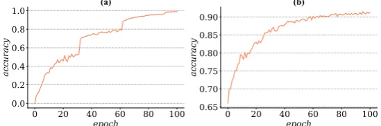
Figure 3.(a) Testing accuracy on mini-ImageNet dataset during pretrain phases for 100 epochs. (b) The accuracy that transfer feature extractor to classify test subset, result shows that model can reach the pretty high accuracy even only trains the classify layer.

0 7 20 60 160 480₁₂80₃₂10₅₁20₉₀50 1536 0 step 50 52 54 56 58 60 62 ac cu ea cy ( % ) (a) normal no sti & no stage

0 7 20 60 160 480 ₁₂80₃₂10₅₁20₉₀50 1536 0 step 50 52 54 56 58 60 62 (b) no stage no sti & no stage

0 7 20 60 160 480 ₁₂80₃₂10₅₁20₉₀50 1536 0 step 72 74 76 78 ac cu ea cy ( % ) (c) normal no sti & no stage

0 7 20 60 160 480₁₂80₃₂10₅₁20₉₀50 1536 0 step 72 74 76 78 (d) no stage no sti & no stage

Figure 4.(a)(b) represent the accuracy results of 5-way 1-shot learning on mini-ImageNet dataset with different settings,no stiin figures means gradient descent is Euclidean gradient,no stageis the setting that disable the multi-stage optimizing method. (c)(d) show results under the setting 5-way 5-shot.

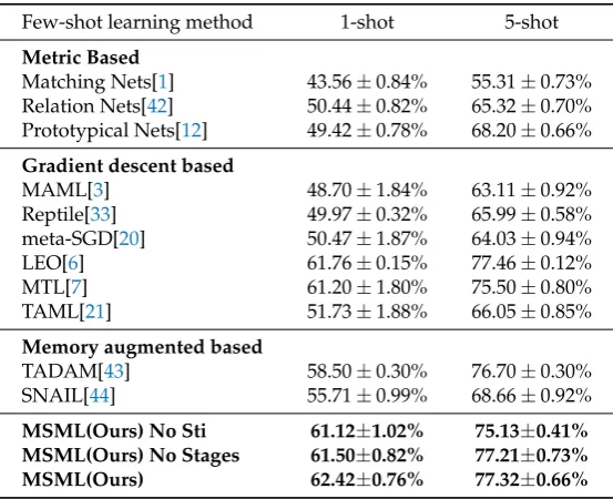
The classification accuracies of our method and other baselines are shown in Table 1. We achieved the state-of-the-art results of the 5-way 1-shot and 5-way 5-shot on mini-ImageNet dataset. Performance of 5-way 1-shot is similar to LEO[6]. Compared with our base model MTL[7], our method proves a certain improvement by using manifold learning approach.

We also present contributions from each method we proposed, results show that deeper network provide significant improvements on feature extraction. The application of Stiefel manifold learning makes the performance of model increase by almost 1% on the basis in 5-way 1-shot learning problem. It’s clear that feature extraction performance reaches the bottleneck when transfer to test set, multi-stage optimization provide tiny improvements to the model. In the setting of machine learning, especially for deep learning, the data in a dataset belong to a certain distribution, which make it possible for neural network to learn the common information from the dataset, but whether these data actually belong to a latent distribution is still unknown, so in a dataset there is a gap on training feature extraction capabilities onsubset1 and applying it tosubset2.

5. Discussion

We introduced three approaches to solve problems of MAML: i) feature extraction; ii) information utilization and iii) the efficiency of gradient descent. By saving intermediate states during adapting processes, we postponed the position of bottleneck to increase the performance of model. Network constrainted to Stiefel manifold offers better descent accuracy. These methods make our model demonstrated the new state-of-the-art result under the setting of 5-way 1-shot and 5-shot.

Table 1. Image classification results on mini-ImageNet under the setting of 5-way 1-shot or 5-way 5-shot. Results in this table reported from their papers.

Few-shot learning method 1-shot 5-shot

Metric Based

Matching Nets[1] 43.56±0.84% 55.31±0.73% Relation Nets[42] 50.44±0.82% 65.32±0.70% Prototypical Nets[12] 49.42±0.78% 68.20±0.66%

Gradient descent based

MAML[3] 48.70±1.84% 63.11±0.92%

Reptile[33] 49.97±0.32% 65.99±0.58%

meta-SGD[20] 50.47±1.87% 64.03±0.94%

LEO[6] 61.76±0.15% 77.46±0.12%

MTL[7] 61.20±1.80% 75.50±0.80%

TAML[21] 51.73±1.88% 66.05±0.85%

Memory augmented based

TADAM[43] 58.50±0.30% 76.70±0.30%

SNAIL[44] 55.71±0.99% 68.66±0.92%

MSML(Ours) No Sti 61.12±1.02% 75.13±0.41% MSML(Ours) No Stages 61.50±0.82% 77.21±0.73% MSML(Ours) 62.42±0.76% 77.32±0.66%

use completely different calculation methods and corresponding learning rates, how to coordinate the step size between the two parts of the model through the adaptive learning rate is also a question to solved. These are works need to be studied in the future to improve the adaptability of model.

6. Materials and Methods

6.1. Computational Requirements

Code used in experiments based on PyTorch and runs on Linux. Softwares required are Python 3.6, CUDA and cuDNN. We recorded the resource usage when running these experiments, program requires 10.1GB GPU memory and 1.8GB memory under the setup of 5-way 5-shot learning.

6.2. Program Availability

Dataset and runnable code used in our experiments are available inhttps://github.com/Chacrk/ MSML_Project, detailed running instructions is also available in repository.

6.3. Running Experiment

Download mini-ImageNet dataset, images are croped to(84×84), unzip file by run command python3 proc_dataset.pyin data folder. Enter directory pretrainand runpython3 pretrain.py to get pretrained weights data.

Pretrain phase last about 5.1 hours by using NVIDIA TITAN Xp and Intel Xeon E5-2620 v4. Enter meta folder while pretrain process done and run commandpython3 main.pyto run the experiment. Author Contributions: All authors contributed to this article, conceptualization, F.D. and F.L.; software, F.D; validation, F.D. and F.L.; writing–original draft preparation, F.D; writing–review and editing, F.D. and F.L.; visualization, F.D.; supervision, F.L.; funding acquisition, F.L.

Funding: This research is supported by National Natural Science Foundation of China under grant number 61902269 and National Key Research and Development Plan "Key Scientific Issues of Transformative Technology" of China(grant number 2018YFA0701701).

Conflicts of Interest:The authors declare no conflict of interest.

References

1. Vinyals, O.; Blundell, C.; Lillicrap, T.; Wierstra, D.; others. Matching networks for one shot learning. Advances in neural information processing systems, 2016, pp. 3630–3638.

2. Szegedy, C.; Vanhoucke, V.; Ioffe, S.; Shlens, J.; Wojna, Z. Rethinking the inception architecture for computer vision. Proceedings of the IEEE conference on computer vision and pattern recognition, 2016, pp. 2818–2826.

3. Finn, C.; Abbeel, P.; Levine, S. Model-agnostic meta-learning for fast adaptation of deep networks. Proceedings of the 34th International Conference on Machine Learning-Volume 70. JMLR. org, 2017, pp. 1126–1135.

4. Arnold, S.M.; Iqbal, S.; Sha, F. Decoupling Adaptation from Modeling with Meta-Optimizers for Meta Learning. arXiv preprint arXiv:1910.136032019.

5. Qiao, S.; Liu, C.; Shen, W.; Yuille, A.L. Few-shot image recognition by predicting parameters from activations. Proceedings of the IEEE Conference on Computer Vision and Pattern Recognition, 2018, pp. 7229–7238.

6. Rusu, A.A.; Rao, D.; Sygnowski, J.; Vinyals, O.; Pascanu, R.; Osindero, S.; Hadsell, R. Meta-learning with latent embedding optimization. arXiv preprint arXiv:1807.059602018.

7. Sun, Q.; Liu, Y.; Chua, T.S.; Schiele, B. Meta-transfer learning for few-shot learning. Proceedings of the IEEE Conference on Computer Vision and Pattern Recognition, 2019, pp. 403–412.

8. Glass, G.V. Primary, secondary, and meta-analysis of research. Educational researcher1976,5, 3–8. 9. Powell, G. A Meta-Analysis of the Effects of" Imposed" and" Induced" Imagery Upon Word Recall.1980. 10. Adey, P.; Shayer, M. Strategies for meta-learning in physics. Physics education1988,23, 97.

11. Koch, G.; Zemel, R.; Salakhutdinov, R. Siamese neural networks for one-shot image recognition. ICML deep learning workshop, 2015, Vol. 2.

12. Snell, J.; Swersky, K.; Zemel, R. Prototypical networks for few-shot learning. Advances in Neural Information Processing Systems, 2017, pp. 4077–4087.

13. Ravi, S.; Larochelle, H. Optimization as a model for few-shot learning2016.

14. Gupta, A.; Eysenbach, B.; Finn, C.; Levine, S. Unsupervised meta-learning for reinforcement learning.

arXiv preprint arXiv:1806.046402018.

15. Nagabandi, A.; Clavera, I.; Liu, S.; Fearing, R.S.; Abbeel, P.; Levine, S.; Finn, C. Learning to adapt in dynamic, real-world environments through meta-reinforcement learning. arXiv preprint arXiv:1803.11347

2018.

16. Al-Shedivat, M.; Bansal, T.; Burda, Y.; Sutskever, I.; Mordatch, I.; Abbeel, P. Continuous adaptation via meta-learning in nonstationary and competitive environments. arXiv preprint arXiv:1710.036412017. 17. Finn, C.; Xu, K.; Levine, S. Probabilistic model-agnostic meta-learning. Advances in Neural Information

Processing Systems, 2018, pp. 9516–9527.

18. Kim, T.; Yoon, J.; Dia, O.; Kim, S.; Bengio, Y.; Ahn, S. Bayesian model-agnostic meta-learning.arXiv preprint arXiv:1806.038362018.

19. Yoon, J.; Kim, T.; Dia, O.; Kim, S.; Bengio, Y.; Ahn, S. Bayesian model-agnostic meta-learning. Advances in Neural Information Processing Systems, 2018, pp. 7332–7342.

20. Li, Z.; Zhou, F.; Chen, F.; Li, H. Meta-SGD: Learning to learn quickly for few-shot learning. arXiv preprint arXiv:1707.098352017.

21. Jamal, M.A.; Qi, G.J. Task Agnostic Meta-Learning for Few-Shot Learning. Proceedings of the IEEE Conference on Computer Vision and Pattern Recognition, 2019, pp. 11719–11727.

22. He, K.; Zhang, X.; Ren, S.; Sun, J. Deep residual learning for image recognition. Proceedings of the IEEE conference on computer vision and pattern recognition, 2016, pp. 770–778.

23. Zhang, Y.; Tian, Y.; Kong, Y.; Zhong, B.; Fu, Y. Residual dense network for image super-resolution. Proceedings of the IEEE Conference on Computer Vision and Pattern Recognition, 2018, pp. 2472–2481. 24. Cai, D.; He, X.; Han, J.; Zhang, H.J. Orthogonal laplacianfaces for face recognition. IEEE transactions on

25. Zhang, Z.; Chow, T.W.; Zhao, M. M-Isomap: Orthogonal constrained marginal isomap for nonlinear dimensionality reduction. IEEE transactions on cybernetics2012,43, 180–191.

26. Fan-Zhang, L.; Huan, X. SO (3) classifier of Lie group machine learning2007. 27. Li, F.z.; Xu, H. SO (3) classifier of Lie group machine learning. Learning2007,9, 12.

28. Nishimori, Y. A Neural Stiefel Learning based on Geodesics Revisited.WSEAS Trans. Syst.2004,3, 513–520. 29. Yang, M.; Li, F.; Zhang, L.; Zhang, Z. Lie group impression for deep learning.Information Processing Letters

2018,136, 12–16.

30. Kingma, D.P.; Ba, J. Adam: A method for stochastic optimization.arXiv preprint arXiv:1412.69802014. 31. Battaglia, P.W.; Hamrick, J.B.; Bapst, V.; Sanchez-Gonzalez, A.; Zambaldi, V.; Malinowski, M.; Tacchetti,

A.; Raposo, D.; Santoro, A.; Faulkner, R.; others. Relational inductive biases, deep learning, and graph networks. arXiv preprint arXiv:1806.012612018.

32. Zagoruyko, S.; Komodakis, N. Wide residual networks.arXiv preprint arXiv:1605.071462016.

33. Nichol, A.; Achiam, J.; Schulman, J. On first-order meta-learning algorithms.arXiv preprint arXiv:1803.02999

2018.

34. Keskar, N.S.; Socher, R. Improving generalization performance by switching from adam to sgd. arXiv preprint arXiv:1712.076282017.

35. Zeiler, M.D. ADADELTA: an adaptive learning rate method. arXiv preprint arXiv:1212.57012012. 36. Bottou, L. Large-scale machine learning with stochastic gradient descent. InProceedings of COMPSTAT’2010;

Springer, 2010; pp. 177–186.

37. Belkin, M.; Niyogi, P. Semi-supervised learning on Riemannian manifolds. Machine learning2004,

56, 209–239.

38. Li, F.Lie Group Machine Learning; Press of University of Science and Technology of China, 2013.

39. Nishimori, Y.; Akaho, S. Learning algorithms utilizing quasi-geodesic flows on the Stiefel manifold.

Neurocomputing2005,67, 106–135.

40. Deng, J.; Dong, W.; Socher, R.; Li, L.J.; Li, K.; Fei-Fei, L. Imagenet: A large-scale hierarchical image database. 2009 IEEE conference on computer vision and pattern recognition. Ieee, 2009, pp. 248–255.

41. Maas, A.L.; Hannun, A.Y.; Ng, A.Y. Rectifier nonlinearities improve neural network acoustic models. Proc. icml, 2013, Vol. 30, p. 3.

42. Sung, F.; Yang, Y.; Zhang, L.; Xiang, T.; Torr, P.H.; Hospedales, T.M. Learning to compare: Relation network for few-shot learning. Proceedings of the IEEE Conference on Computer Vision and Pattern Recognition, 2018, pp. 1199–1208.

43. Oreshkin, B.; López, P.R.; Lacoste, A. Tadam: Task dependent adaptive metric for improved few-shot learning. Advances in Neural Information Processing Systems, 2018, pp. 721–731.