Article
Time Evolving Undirected Graphical Model for
Protein-Protein Interaction Networks
Yasanthi Malika Hirimutugoda1
1 Department of Information Technology, Sri Lanka Institute of Advanced Technological Education, Sri Lanka * Correspondence: [email protected]
Abstract: Proteins are the workhorses of the cell that perform biological functions by interacting with other proteins. Many statistical methods for protein-protein interaction (PPI) have been studied without considering time-dependent changes in networks and the functionalities. I introduced a novel method that models PPI networks as being dynamic in nature and evolving time-varying multivariate distribution with Conditional Random Fields (CRF). This research is directed towards implementing this new combinatorial algorithm on massively parallel architectures such as Graphics Processing Units (GPUs) for efficient computations for large scale bioinformatics datasets. I compared Conditional Random Fields (CRF) and the proposed novel method using CRF combined with the Block Coordinate Descent algorithm for human protein-protein interaction data set. Both are implemented on GPU-Accelerated Computing Architecture and the proposed novel method showed the advantages in predicting protein-protein interaction sites.I also show that the proposed approach is more efficient in 6.13% than standalone CRF++ in predicting protein-protein interaction sites.
Keywords: Proteins, time-varying, parallel, architectures, Conditional Random Fields (CRF), Graphics Processing Units, Block Coordinate Descent algorithm
Introduction:
Proteins are the molecular machinery of life. The living cell is made of proteins. All data in biological system are processed, integrated, and executed through complex interactions networks. Protein-Protein Interaction Network (PPIN) generates various kind of relationships between proteins, such as physical interactions, regulatory and metabolic pathways, similarity in sequence motifs, gene expression profiles, cellular localization etc.,[1].
In PPIN, proteins correspond to nodes and relationships between proteins correspond to edges. With highly non-linear relationships and rapid dynamics, these networks are a complex system. Also PPINs generate topological structures, complex functions and dependencies, including hierarchical structures, multiple types of edges, but these structures and dependencies are weakly understood, poorly characterized, and more challenging, if dynamic nature is not considered [1].
However, the complexity in biological networks is often approached in a static and time-invariant manner without considering rapidly changing regulatory mechanisms as well as acquired evolutionary relationships between proteins. Such approaches describe that network relationships happen only at an instant during the evolution of system. Such time-dependencies in the PPIN can entirely redefine network topology with completely different functional relationships between proteins at various times and states of the system. These time-dependent functional and topological changes in the network are crucial for identifying malfunctioning regulatory pathways at different disease stages [2, 3]. Real-time analysis of PPIN is important for detecting anomalies, predicting border. Real-time analysis of PPIN is important for detecting anomalies, predicting vulnerability, and assessing the potential impact of interventions in biological systems.
With increasing vast amounts of data in PPI networks, performance and scalability issues are becoming a critical limiting factor [4, 5]. Because of that, it is important to find a solution for its high performance and efficiency.
The main objective of this study is to build a fast parallel time-varying graphical model for a large scale protein-protein interaction networks to address above issues. By considering functions of biological building blocks such as proteins, genes, small molecules, protein complexes etc, the next
attempt is to create a general model that can map with the topologies of these dynamically change biological networks. My last objective is to build a solution for performance and efficiency for large scale data set.
Related Work and Overview
A PPI network can be described as a complex system of proteins linked by interactions. The computational analysis of PPI networks begins with the representation of the PPI network structure. The simplest representation takes the form of a mathematical graph consisting of nodes and edges. Proteins are represented as nodes in such a graph; two proteins that interact physically are represented as adjacent nodes connected by an edge. Based on this graphic representation, various computational approaches, such as data mining, machine learning, and statistical approaches, can be designed to reveal the organization of PPI networks at different levels. An examination of the graphic form of the network can yield a variety of insights [6].
In 2006, Chung investigated that this relation and used the clustering as a post-processing strategy to remove the isolated interface residues predicted by SVMs, and included the noninterface residues surrounded by several predicted interface residue [7]. Before this, several researches have successfully applies many machine learning method such as SVM, Neural Networks.
In 2006, Conditional Random Fields has been successfully applied by Sutton to solve sequence labeling problems, and are also proved their effectiveness in solving problems in protein secondary structure prediction and protein fold recognition [8].
In 2011, Morihiro Hayashida proposed a novel method which combines conditional random fields with the domain based model of protein-protein interactions. Furthermore, they have improved the method by introducing mutual information. In order to give better performance, they have introduced mutual information to the probabilistic model [9].
In contrast, in recent years, high throughput view of the PPI consider proteins as logical entities and they represent their interactions as a network but statically without considering time-dependent changes in the network and the functionality.
In 2008, Shuheng Zhou has shown how to estimate the sequence of graphs for non-identically distributed data, where the distribution evolves over time. In this paper, they have developed a nonparametric method for estimating time varying graphical structure for multivariate Gaussian distributions [10].
In 2011, Jun Sung Joon has presented a fast parallel implementation using commodity graphics hardware based a well-known sequential complex finding algorithm to address the computational challenge. This parallel algorithm is implemented on the NVIDIA parallel computing architecture of CUDA. It is evaluated for a various kinds of large-scale PPI networks [11]. In the same year, Alhadi Bustamam has introduced a very fast Markov clustering algorithm (MCL) using CUDA to perform parallel sparse matrix-matrix computations and parallel sparse Markov matrix normalizations, which are at the heart of MCL. They have utilized sparse format to allow the effective and fine-grain massively parallel processing to cope with the sparse nature of interaction networks datasets in bioinformatics applications [12].
In 2009, Ming-Hui Li and Lei Lin have mentioned and proved, CRF is the best way to model biological networks like PPINs. The advantage of CRFs is that it can integrate both rich state features and transition features between label states. Furthermore, CRFs have advantages over traditional graphical models such as hidden Markov models (HMMs) and maximum entropy Markov models (MEMMs). It is one of the outstanding methods used for labeling sequence data [13].
PPI have been studied in different perspectives. In the classical view, PPI prediction has been studied as a classification task and separately studied each residue, so one interface residue is identified at a time. The disadvantage of these methods is the relation between two labels of neighboring residues is not considered. However, sequentially or spatially neighboring residues should have similar characters in building interfaces [16,17].
Markov Cluster Algorithm, a fast and scalable unsupervised cluster algorithm for networks (also known as graphs) based on simulation of flow in graphs. Also Markov Clustering Algorithm has been used to with CUDA for data networks. As this algorithm is based on the graph theory, parallel computing architecture.
Research Methodology and Algorithms
Graphical models are a marriage between probability theory and graph theory. The graphical model is the fundamental solution to model a complex system by combining simpler parts. Probability theory provides the glue whereby the parts are combined, ensuring that the system as a whole is consistent, and providing ways to interface models to data. The graph theoretic side of graphical models provides both an intuitively appealing interface by which humans can model highly-interacting sets of variables as well as a data structure that lends itself naturally to the design of efficient general-purpose algorithms [13].
Network models are the most popular way to represent complex systems by considering the relational patterns among observed variables. In various research areas such as biology, astronomy and social sciences, successful network models are based on the Gaussian graphical models (GGMs).The precision matrix represents conditional dependencies between random variables and a network representation is obtained by linking conditionally dependent variables in the framework of the GGMs. This graphical representation provide additional insight into the system under observation by showing how different parts of the system interact. [18]
CRF is the best graphic representation to model biological networks like PPINs on the above review. The advantage of CRFs is that it can integrate both rich state features and transition features between label states. It is one of the outstanding methods used for labeling sequence data. In my study, each residue needs to be labeled as an interface residue or noninterface residue in given a protein sequence with structural information. Furthermore, considering advantages of CRFs over traditional graphical models such as hidden Markov models (HMMs) and maximum entropy Markov models (MEMMs), the CRF was used rather than other graphical models. [17,23].
Markov Cluster Algorithm, a fast and scalable unsupervised cluster algorithm for networks (also known as graphs) based on simulation of flow in graphs[19]. Also Markov Clustering Algorithm has been used to with CUDA for data networks. As this algorithm is based on the graph theory, parallel computing architecture can be applied to model my approach.
1. Undirected Graphical Model
A graph consists of a set of vertices (nodes), along with set of joining some pairs of the vertices. In graphical models, each vertex represents a random variable, and the graph gives a visual way of understanding the joint distribution of the entire set of random variables [20].
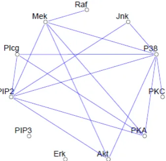
Figure 1 Example of a sparse undirected graph, estimated from a flow cytometry dataset, with p = 11 proteins measured on N = 7466 cells. The network structure was estimated using the graphical lasso procedure
In these graphs, the absence of an edge between two vertices has a special meaning: the corresponding random variables are conditionally independent, given the other variables [20].
Figure 1shows an example of a graphical model for a flow-cytometry dataset with p = 11 proteins measured on N = 7466 cells. Each vertex in the graph corresponds to the real-valued expression level of a protein.The network structure was estimated assuming a multivariate Gaussian distribution, using the graphical lasso procedure [21].
1.1. Markov Graphs and Their Properties
Figure 2 shows four examples of undirected graphs. A graph G consists of a pair (V,E), where V is a set of vertices and E the set of edges (defined by pairs of vertices).Two vertices X and Y are called adjacent if there is an edge joining them; this isdenoted by X ∼ Y.
A path X1, X2, . . . ,Xn is a set of vertices that are joined, that is X i−1 ∼ Xi for i = 2, . . . , n. A complete graph is a graph with every pair of vertices joined by an edge. A subgraph U ∈ V is a subset of vertices togetherwith their edges.
In a Markov graph G, the absence of an edge implies that the corresponding random variables are conditionally independent given the variables at the other vertices. This is expressed with the following notation:
For example, (X, Y,Z) in Figure 2(a) form a path but not a complete graph [20]. No edge joining X and Y ⇐⇒ X ⊥ Y |rest
Where “rest” refers to all of the other vertices in the graph. For example in Figure 2(a), X ⊥ Z|Y. These are known as the Pairwise Markov Independencies of G [20].
In a Markov graph G with sub-graphs A, B and C, if C separates A and B then A ⊥ B|C.
A probability density functionf over a Markov graph G can be can represented as Eqn. 1
Where C is the set of maximal cliques, and the positive functions ψC(·) are called clique potentials. These are not in general density functions, but rather are affinities that capture the dependence in XC by scoring certain instances XC higher than others. The quantity is the normalizing constant, also known as the partition function. Alternatively, the representation (Eqn. 1) implies a graph with independence properties defined by the cliques in the product.This result holds for Markov networks G with positive distributions, and is known as the Hammersley Clifford Theorem [22, 25].
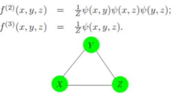
A graphical model does not always uniquely specify the higher-order dependence structure of a joint probability distribution. Consider the complete three-node graph in Figure 3. It could represent the dependence structure of either of the following distributions as equation 3 and 4.
Figure 3. A complete graph does not uniquely specify the higher-order dependence structure in the joint distribution of the variables.
The Eqn.2 specifies only second order dependence (and can be represented with fewer parameters). Graphical models for discrete data are a special case of log linear models for multiway contingency tables [24] in that language
f
(2) is referred to as the “no second-order interaction” model.1.2. Conditional random field model for PPI
1.2.1. Conditional random fields used for labeling sequence
CRF has a single exponential model for the joint probability of the entiresequence of labels given the observation sequence. Conditional random fields (CRFs) were proposed for labeling sequence data [16].
Protein surface residues were extracted and the surface residue segments were treated as sequence data. Residues on surface segments were labeled as interface or noninterface residues using Conditional Random Field [17].
The graphical model representation for chain-form CRFs is shown in Fig. 5, where we have one state assignment for each residue in the sequence. Especially the conditional probability P(Y/X) is defined as Equation 5.
(1)
(2)
(3)
(4)
Where fk can be arbitrary features, including overlapping or long-range interaction features. Given a sequence of observations X = (x1, x2, …, xn), we want to get the most probable label sequence Y = (y1, y2, …, yn), i.e.The parameters λ = (λ1……..λk) are computed by minimizing the regularized log-loss of the conditional probability of the training data [26].
Figure 5: Graphical model representation of and chain-structured CRF 1.3 Time-arraying probabilistic graphical model with PPI Networks
The time-varying multivariate Gaussian distribution and the undirected graph associated with it provide a useful statistical framework for modeling complex dynamic networks.
A stationary undirected probabilistic graphical model (PGM), also known as a Markov Random Field, is a tuple M= (V; E; F). Here V is a set of nodes corresponding to a collection of random variables, E is a set of undirected edges encoding them conditional independencies between random variables, and F is a set of functions, also known as factors, on the nodes and edges. A Markov Random Field factors the joint distribution as the products of the factors. When each random variable is distributed according a Gaussian distribution, it is called Gaussian Graphical Model (GGM) [27,28].
We can extend the stationary model to the time varying case by making the set of edges and the parameters of the functions a function of t. That is, our model has the form: M(t) = (V;E(t); F(t)). First parameter estimation of a regularized Gaussian Graphical Model studied and extended to the algorithm to learn the time varying GGM [28].
1.4 Multivariate Gaussian Graphical Models
Gaussian Graphical Models are multivariate probability distributions encoding a network of dependencies among variables. Let θ = [θ1; θ2; ::; θn] be a set of n variables, and let f(θ=D) be the value of the probability density function at a particular value D[28,34].
A multivariate GGM factors this as in Equation 6.
Where Z is the normalization coefficient. The parameters of this distribution are µ and ∑ [27,28].
1.5 Regularized Time Varying Gaussian Graphical Model
1.5.1 Convex Optimization for Parameter Estimation of Regularized Time Varying GGM
Let D 1..T(1)…(m) be the set of training data, where each Dt(i) is a sample represented by n variables. The time varying GGM parameter estimation algorithm extends the stationary GGM parameter learning as follows in equation 7 [28].
Here, S(t) is the weighted covariance matrix, and is calculated as follows in equation 8.
The weights wst are defined by a symmetric nonnegative kernel function. As a kernel with a larger span will cause the time varying model to be less sensitive to abrupt changes in the network and capture the slower and more robust behaviors. On the other hand, as the kernel function span decreases, the time varying will be able to capture more short term patterns of interaction [28].
(6)
(7)
I used Block Coordinate Descent Algorithm to solve the stationary and time varying problems. This method has been proposed by Banerjee [41], and proceeds by forming the dual for the optimization case, and applying block coordinate descent to the dual form [28].
Recall that the basic form of both the stationary and time varying case is as follows in equation 9.
We first rewrite the L1-norm as:∞
In equation 10, where ||U||∞ denotes the maximum absolute value element of the matrix U. Given
this change of formulation, we can rewrite the primary form of the problem as in equation 11.
Thus, the optimal ∑-1 is the one that maximizes the worst case log likelihood, over all additive perturbations of the covariance matrix, S [28].
Next, to obtain the dual form, we exchange the min and max, and the inner max objective function can now be solved analytically taking the gradient and setting it to zero. This results in the new form of the objective function:
Where n is the number of features in each sample.
Once we solve this problem, the optimal ∑-1 can be computed as ∑-1 = (S + U*)-1. Performing one last change of variables W = S +U, and forming the dual of the problem will bring us to the final form of our objective.
1.5.2 The Block Coordinate Descent Algorithm
For any matrix A, let A\k\j denote the matrix produced by removing column k and row j of the matrix. Let Aj also denote the column j, with diagonal element Ajj removed. The Block Coordinate Descent algorithm proceeds by optimizing one row and one column of the variable matrix W at a time. The algorithm iteratively optimizes all columns until a convergence criteria is met. The algorithm as follows [28,29].
The W(j)s produced in each step are strictly positive definite. This property is important because the dual problem estimates the covariance matrix ∑, rather than the inverse covariance matrix, ∑-1,
The network conditional dependencies which we are interested in are encoded in the inverse covariance matrix, so the strictly positivity of W(j) will guarantee that the optimum ∑ will be reversible, and that we can compute the final answer ∑-1 from the W(j) [28]
2. Graphics processing units (GPUs) for large-scale protein interaction networks
A protein-protein interaction network is represented as proteins are nodes and interactions between proteins are edges. Protein complexes and functional modules can be identified as highly interconnected subgraphs and computational methods are now inevitable to detect them from protein interaction data. As the interaction dataset increases, the scale of interconnected protein networks
(9)
(
10)(11)
(12)
increases exponentially so that the increasing complexity of network gives computational challenges to analyze the networks[11,30].
Markov clustering (MCL) is becoming a key algorithm within bioinformatics for determining clusters in networks [17]. Here I used "Molecular Complex Detection" (MCODE) algorithm also makes the visualization of large networks manageable by extracting the dense regions around a protein of interest. The MCODE algorithm operates in three stages, vertex weighting, complex prediction and optionally post processing to filter or add proteins in the resulting complexes by certain connectivity criteria [30].
This MCODE algorithm has the advantage over other graph clustering methods of having a directed mode that allows fine-tuning of clusters of interest without considering the rest of the network and allows examination of cluster interconnectivity, which is relevant for protein networks [30]. Parallel MCODE Algorithm for protein Complex Prediction
d: vertex weight percentage Wv: vertex weight of v
S
v: vertex weight of seed of vNv : seed vertex of v Sv← v, for all v
while there is any changes of Sv for all v neighbors of n do in parallel if Nv <> Nn then
if Wv < Sn AND Wv> (1-d) Sn then Sv ← Sn
Nv ← Nn
else if Wv = Sn AND Cv > Cn then Nv ← Nn
end if end if
synchronize all threads end while
3. Data and Implementation
The Human protein-protein interaction data file “Hsapi20170205.txt” from DIP database was used [32, 33] for analyzing. All DIP database records available through this Web Site are freely available under the terms set by the Creative Commons Attribution-NoDerivs License [33]. Initially I started with 9025 number of protein interactions entries of Homo sapiens which are given in Hsapi20170205.txt file of DIP database. As some entries among these interactions were not matched with their primary sequences, the multi-stage refinement was applied to remove the interactions with incomplete information. After processing them step by steps it was reduced uptown 168 in our Homo sapiens training dataset. [33].
CRF++ is a simple, customizable, and open source implementation of Conditional Random Fields (CRFs) for segmenting/labeling sequential data. CRF++ is designed for generic purpose and will be applied to a variety of NLP tasks, such as Named Entity Recognition, Information Extraction and Text Chunking [36].
Table 1: Results for training and test datasets using the CRF model and our novel model for human computer data for mutual information protein interactions
Training Recognitio n of Testing
Testing Recognition of Testing
1 98.31% 74.51% 98.45% 84.92%
2 98.81% 74.67% 97.57% 82.72%
3 93.45% 84.02% 98.59% 83.93%
Average 96.86% 77.73% 98.23% 83.86%
CRF++, less memory usage both in training and testing, has been written in C++ with STL. By combining the two approaches CRF++ and Block Coordinate Descent algorithm using C++, I obtained an implementation that is very competitive and often outperforms other state-of-the-art approaches for this problem. I also show that the proposed approach is more efficient in practice than the one implemented in standalone CRF++ for human protein data set.
Both were implemented on GPU-Accelerated Computing Architecture. AllegroMCODE plugin, a well-known molecular complex detection tool was integrated in the open-source network visualization and analysis platform of Cystoscape platform [30]. This parallel MCODE algorithm is implemented on the NVIDIA parallel computing architecture of CUDA [11].
4. Result
In order to evaluate our method, I compared two models, the CRF and proposed method CRF with the Block Coordinate Descent algorithm. Both models were implemented GPU-Accelerated Computing Architecture. Table 1 shows the results for training and test datasets using the CRF model and our novel model for human computer data for mutual information protein interactions.
5. Conclusion
Conditional Random Fields (CRF) and the proposed novel method which combines CRF with the Block Coordinate Descent algorithm were compered for Human Protein interaction Data with mutual information. Both are implemented on GPU-Accelerated Computing Architecture and the proposed novel method show more efficiency in 6.13% than standalone CRF in predicting protein-protein interaction sites .
Acknowledgements: I would like to thank all the people in my academic and personal life who motivated, supported, and, most importantly, believed in me. Further, I would like to extend thank my former research advisor Dr G Wijerathne whose encouragement, and advice have been a driving force of my work. Also I would like to extend my thanks to SLIATE by providing the research grant according to the DMS circular for encouraging our research culture.
References
[1] Jonathan Pevsner (2009) Second Edition, Bio informatics and functional Genomic,
[2] Joaquín Goñi, Francisco J Esteban, Nieves Vélez de Mendizábal, Jorge Sepulcre, Sergio Ardanza-Trevijano, Ion Agirrezabal and Pablo Villoslada (2008) A computational analysis of protein-protein interaction networks in neurodegenerative diseases, BMC Systems Biology.
[3] C. M. Schneider ,R.F.S.Andrade ,T.Shinbrot and H. J. Herrmann (2011) The fragility of protein-protein interaction networks
[4] Alhadi Bustamam (2011) Modelling Static Networks in Bioinformatics Applications Using Advanced Computing.
[5] V. Spirin and L. A. Mirny,(2003) “Protein complexes and functional modules in molecular networks,” Proceedings of the National Academy of Sciences of the United States of America, vol. 100, no. 21, pp. 12123– 12126
[6] Aidong Zhang (2009) State university of New York, Protein Interaction Networks Computational Analysis [7] Jo-lan Chung, Wei Wang, Philip E. Bourne (2006) Exploiting sequence and structure homologs to identify
[8] Sutton C, McCallum (2006) An introduction to conditional random fields for relational learning. In: Getoor L, Taskar B, editors. Introduction to Statistical Relational Learning. MIT Press, Cambridge, Massachusetts, USA; [9] Morihiro Hayashida, Mayumi Kamada, Jiangning Song, and Tatsuya Akutsu, (2010) Conditional random field
approach to prediction of protein-protein interactions using domain information,China
[10]Shuheng Zhou, John D. Lafferty, and Larry A. Wasserman. (2008) Time varying undirected graphs. In COLT, pages 455–466
[11]Jun Sung, Yoon, Won Hyong, GPU-accelerated Bioinformatics Application for Large-scale Protein Interaction Networks
[12]Alhadi Bustamam , Kevin Burrage, Nicholas A. Hamilton, Fast Parallel Markov Clustering in Bioinformatics using Massively Parallel Computing on GPU with CUDA and ELLPACK-R Sparse Format
[13]Ming-Hui Li, Lei Lin, Xiao-Long Wang and Tao Liu (2007) Bioinformatics Research Group, ITNLP Lab, Protein–protein interaction site prediction based on conditional random fields, Department of Computer Science and Technology, Harbin Institute of Technology, Harbin, China.
[14]Micheal I Jordan (1986) Serial Order: A Parallel Distributed Processing Approach, Institute of Cognitive Science, Calilifonia
[15]Chia, J.M., Kolatkar, P.R.: (2004) Implications for domain fusion protein-protein interactions based on structural information. BMC Bioinformatics 5, 161
[16]Espadaler, J., Romero-Isart, O., Jackson, R., Oliva, B. (2005) Prediction of protein-protein interactions using distant conservation of sequence patterns and structure relationships. Bioinformatics.21(16), 3360–8
[17]John Lafferty, Andrew McCallum, Fernando C.N. Pereira (2001) Conditional Random Fields: Probabilistic Models for Segmenting and Labeling Sequence Data, Proceedings of 8th International Congress on machine learning, pages 282-289
[18]Michael Jordan (1998) Learning in Graphical Models
[19]Mladen Kolar, Eric P. Xing, On Time Varying Undirected Graphs.
[20]Trevor Hastie, Robert Tibshirani, Jerome Friedman (1993) The Elements of Statistical Learning, Data Mining, Inference, and Prediction,
[21]Sachs, K., Perez, O., Pe’er, D., Lauffenburger, D. and Nolan, G. (2003). Causal protein-signaling networks derived from multipara meter single-cell data, Science 308(5721): 523–529.
[22]Samson Cheung (2008) Proof of Hammersley-Clifford Theorem
[23]Lafferty, J (2001) Conditional Random Fields: Probabilistic Models for Segmenting and Labeling Sequence Data. 18th International Conference on Machine Learning (ICML). 282-289.
[24]Bishop, Y., Fienberg, S. and Holland, P. (1975). Discrete Multivariate Analysis, MIT Press, Cambridge, MA. [25]Hammersley, J. M. and Clifford, P. (1971). Markov field on finite graphs and lattices, unpublished.
[26]Yan Liu (2005) Conditional Graphical Models for Protein Structure Prediction.
[27]Franz Pernkopf, Robert Peharz, Sebastian Tschiatschek, (2014) Introduction to Probabilistic Graphical Models [28]Narges Sharif Razavian, Subhopdeep Moitra, Hetunandan Kamisetty, Arvind Ramanathan, Christopher
James Langmead (2010) Time-varying Gaussian Graphical Models of Molecular Dynamic Data, Carnegie Mellon University, Pittsburgh.
[29]Zhiwei Qin , Katya Scheinberg, Donald Goldfarb (2013) Efficient block-coordinate descent algorithms for the Group Lasso, Springer-Verlag Berlin Heidelberg and Mathematical Optimization Society.
[30]G. D. Bader and C. W. V. Hogue (2003) "An automated method for finding molecular complexes in large protein interaction networks", BMC Bioinformatics, 4(2), 2003
[31]Fort Lauderdale, FL, USA. Volume 15 of JMLR: W&CP 15. (2011). Appearing in Proceedings of the 14th International Conference on Artificial Intelligence and Statistics (AISTATS),
[32] L. Salwinski, C. S. Miller, A. J. Smith, F. K. Pettit, J. U. Bowie, and D. Eisenberg. (2004) The Database of Interacting Proteins: 2004 update. Nucleic Acids Research, 32:D449–D451
[33]http://dip.mbi.ucla.edu/dip/download?mst=1:2:5&tbs=5:0, DIP Archival Datasets [34]Philip Bachman, Doina Precup, Improved Estimation in Time Varying Models,
[36]https://taku910.github.io/crfpp/, CRF++: Yet Another CRF toolkit
[37]Guangyu Cui,Y u Chen, De-Shuang Huang and Kyungsook Han (2007) An Algorithm for Finding Functional Modules and Protein Complexes in Protein-Protein Interaction Networks, Journal of Biomedicine and Biotechnology,South Korea
[38]Amr Ahmed, Le Song, Eric P, Xing (2008) Time-Varying Networks: Recovering Temporally Rewiring Genetic Networks During the Life Cycle of Drosophila melanogaster,USA
[39]Xenarios I, Salwinski L, Duan XJ, Higney P, Kim S, Eisenberg D (2002) DIP: The Database of Interacting Proteins. A research tool for studying cellular networks of protein interactions.
[40]Brijesh K. Sriwastava , Subhadip Basu, Ujjwal Maulik, Dariusz Plewczynski (2013) PPIcons: identification of protein-protein interaction sites in selected organisms.