Simulation of the supply capability of sheep on the Mitchell grass downs of north west Queensland

Full text

(1)Simulation of the Supply Capability of Sheep on the Mitchell Grass Downs of North West Queensland P.M. Peppera, L.B. Dunlopb, E.J. Westonc and D. Cloonand a. Agency for Food and Fibre Sciences, Queensland Department of Primary Industries, Locked Mail Bag No. 4, Moorooka Q4105. ([email protected]). b. Agency for Food and Fibre Sciences, Queensland Department of Primary Industries, Locked Mail Bag No. 2, Goondiwindi Q4390. ([email protected]) c. d. Agency for Food and Fibre Sciences, Queensland Department of Primary Industries, P.O.Box 102, Toowoomba Q4350. ([email protected]) Agency for Food and Fibre Sciences, Queensland Department of Primary Industries, G.P.O.Box 46, Brisbane Q4001. ([email protected]). Abstract: Sheep in western Queensland have been predominantly reared for wool. When wool prices became depressed interest in the sheep meat industry, increased. For north west Queensland producers, opportunities may exist to participate in live sheep and meat export to Asia. A simulation model was developed to determine whether this sheep producing area has the capability to provide sufficient numbers of sheep under variable climatic conditions while sustaining the land resources. Maximum capacity for sustainability of resources (as described by stock numbers) was derived from an in-depth study of the agricultural and pastoral potential of Queensland. Decades of sheep production and climatic data spanning differing seasonal conditions were collated for analysis. A ruminant biology model adapted from Grazplan was used to simulate pregnancy rate. Empirical equations predict mortalities, marking rates, and weight characteristics of sheep of various ages from simple climatic measures, stocking rate and reproductive status. The initial age structure of flocks was determined by running the model for several years with historical climatic conditions. Drought management strategies such as selling a proportion of wethers progressively down to two-tooth and oldest ewes were incorporated. Management decisions such as time of joining, age at which ewes were cast-for-age, wether turn-off age and turning-off rate of lambs vary with geographical area and can be specified at run time. The model is run for sequences of climatic conditions generated stochastically from distributions based on historical climatic data correlated in some instances. The model highlights the difficulties of sustaining a consistent supply of sheep under variable climatic conditions. Keywords: Sheep; Supply capability; Variable climate; Simulation. 1.. INTRODUCTION. As wool prices became depressed in 1994, the possibility of wool producers in north west Queensland participating in the live sheep and meat export to Asia was raised. From May to August supplies from southern States are low and cast-for-age sheep and young wethers could find a market if sufficient numbers of acceptable quality could be supplied. In north west Queensland, native pastures provide the major source of feed although there is some potential for increasing the livestock carrying capacity through. the development of sown pastures [Weston et al., 1981]. Climate variability has a major influence on the capability of the sheep industry to provide a consistent quality product. The rangelands are shared with the beef industry and movement between the two industries largely depends on This paper describes the economics. development of a model simulating the age structure and weight of the flocks depending on the season. The numbers of ewes and wethers simulated are compared with historical ABS data [Australian Bureau of Statistics, 1960 to 1997] for.

(2) the sheep producing shires (Cloncurry, Flinders, McKinlay and Richmond) in the north west Queensland Division (NW). Sequences of climatic conditions are generated stochastically from distributions based on historical climatic measures to investigate the supply capability under different management strategies.. 2.. 2.3 Prediction of Liveweight and Liveweight Gain/Loss of Ewes and Wethers in Various Age Classes Data from field trials [Jordan et al., 1989; Rose and Young, 1988] were analysed by multiple regression to predict fleece free liveweight (kg) at joining for ewes of age i in season j.. METHOD OF MODEL DEVELOPMENT Wij= 42.8 – 0.0341dayj-1 + 0.0144rdjj+ 3.01agei – 0.250agei2 (2). 2. 1 Description of Seasons Simple climatic measures derived from meteorological data (Table 1) were used to describe the seasons. These measures were included as possible predictors in the empirical equations estimating reproduction, mortalities and weight of sheep of various age classes.. 2.2 Generation of Seasons From 39 years of meteorological data from Toorak Sheep Field Research Station, means, µ, standard deviations, σ, and correlations, ρ, were determined for the climatic measures. As the distribution of rainfall was skewed, logarithms of rainfall were taken. Values for two correlated climatic measures, Y1 and Y2, were generated as follows [Tocher, 1963]:Y1 = µ1 + σ1r1 Y2 = µ2 + σ2(r1ρ + r2√(1 – ρ2)). (1). where r1 and r2 were two random variates from a normal distribution with a mean of zero and standard deviation of one. In this way any number of years of seasons could be simulated.. where agei = 1.5,2.5 …..age cast-for-age (years). The predictor variables explained 82% of variation in weight of ewes in the field trials. Stocking rate was not included as a predictor as ewes grazed at the district average stocking rate. As there could be potential for Queensland producers to sell wethers during winter months, empirical equations to predict the May weight of wethers (WWij; kg) of age i for season j and the rate of gain/loss in weight from May to September (ADGij; kg/day) were calculated using data from field trials [McMeniman et al., 1986; Phelps et al., 1994]. WWij= 21.4 + 0.0265rdwj + 0.0155rdj-1 + 0.18agei + 0.481agei2 – 2.26SRj (3) ADGij= – 0.0653 – 0.0102agei + 0.00481rddaysj – 0.0156SRj (4) where SRj= dry sheep equivalents/ha for season j.. Table 1. Climatic measures derived from Toorak Sheep Field Research Station, Julia Creek (Latitude 21o 2’ Longitude 141o 48’) and used for NW Queensland. Measure Description Mean Min. Max. rdj. rdwj rdjj dayj-1 rddaysj rdbreak. Rainfall, mm, in the current growing season i.e. year j. Beginning of the growing season was defined as first date after 1 July when the sum of the rain over three days was greater than 10 mm and the average temperature greater than 140C. End of season was specified by the date of the last similar event before 30 June of the next year rainfall, mm, in the current growing season prior to May rainfall, mm, in the current growing season prior to start of joining days from end of previous growing season to mid-joining period number of rain days in the growing period if current season breaks, rainfall from that time to mid joining eg if joining is in November and there are early storms, the growing season is still defined as the previous spring summer and the rainfall since the first significant event to mid-joining recorded as a separate variable; Probability of early storms = 0.33.. 392. 112. 1251. 372 392 582 27 49. 112 112 504 10 10. 1217 1251 664 59 153.

(3) The predictor variables explained 72% of variation in wether weight and 39% of variation in average daily gain/loss of the field trials.. removals occurred were used to determine equation (8) which explained 36% of variation:MR = 1/(1+e-y); y = – 3.00+0.943SRj. 2.4 Prediction of Marking Rate of Ewes of Different Age Classes While pregnancy rates could be predicted satisfactorily from a process model [Freer et al., 1997; Pepper et al., 1999], prenatal and post-natal losses were difficult to predict. Hence, empirical equations were fitted to field data [Rose, 1976; Jordan et al., 1989] to predict marking rate (MARij ) from climatic measures and age of the ewes. MARij= 0.295 – 0.0007dayj-1 + 0.00998rddaysj + 0.144agei – 0.0141agei2. (5). Equation (5) explained 71% of variation of marking rate of the field data.. 2.5 Prediction of Mortalities of Wethers of Various Ages. Ewes and. The mortalities between joinings for ewes aged 1.5 years and over were determined using data from field trials [Jordan et al., 1989; Rose, 1976]. MRij =1/(1+e-y);. In the model, mortalities were estimated as the maximum of MR and MRij.. 2.6 Adjustments for Flooding, Pests and Predators Unusually severe flooding as occurred in the 1974/75 season was programmed into the model by assuming an increase in mortality of k1 and a decrease in marking rate of k2. Such a flood was assumed to occur if: > mean(rddaysj) + 2.33standard rddaysj deviation(rddaysj) and log(rdj ) > mean(log(rdj)) + 2.33standard deviation(log(rdj)). Such a flood would be an extremely unlikely event (Probability <0.01). In a run of good seasons, parasites and predators such as pigs can build up causing the marking rate to be lower than the expected rate. Therefore mortality rate of weaners was assumed to increase by pest factors (k3) and (k4) and marking rate to reduce by (k31) and (k41) respectively under the following conditions:rddaysj for two consecutive seasons ≥ the 90% quantile of historical data - pest factors (k3), (k31). y = – 1.80 – 0.776agei+ 0.0995agei2 + 2.18pri –0.00242rdj-1. (8). (6). where pri = pregnancy rate of ewes aged i years estimated from the process model which is dependent on time of joining and weight of the ewe [Freer at al., 1997; Pepper et al., 1999]. Equation (6) explained 66% of variation in mortalities in the field trials. Mortalities from marking to first joining were estimated from limited data from field trials at Toorak Research Station [Rose, 1972].. rddaysj for three consecutive seasons ≥ the 70% quantile - pest factors (k4), (k41) rddaysj for two consecutive seasons ≥ the 70% quantile and rain in spring (rdbreak > 0 for spring joining) - pest factors (k4), (k41) rddaysj for season ≥ the 90% quantile and previous year a pest year - pest factors (k4), (k41) If there is spring rain in the year after a flood, pest factors (k3) and (k31) are assumed.. MR1j = 1/(1+e-y); y = 0.295 – 0.102rddaysj. (7). Equation (7) explained 64% of the variation. One estimate of mortalities of wethers was determined from equation (6) setting pri to zero. Few mortality data are available from research data as measures are taken to avoid stock deaths. However some data were available from a utilisation trial [Phelps et al., 1994] in which animals weighing less than 30 kg were removed from the trial. Data from treatments in which. 2.7 Drought Strategies In a drought year the strategy of selling off a proportion k5 of wethers aged over 1.5 years and reducing the number of ewes joined by a factor k6 was assumed. A drought year was defined as follows:rdj and rdj-1 < the 20% quantile and dayj-1 > the 80% quantile of historical data rdj < the 10% quantile of historical data.

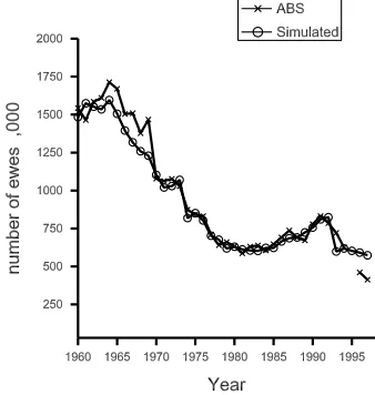
(4) 2.8 Sustainable Livestock Capacity An estimate of sustainable livestock capacity expressed as dry sheep equivalents (SDSE) was obtained from Weston et al. [1981]. Using the area of native and sown pasture in each of 13 vegetation zones which occur in the identified shires, and a stocking rate considered to be sustainable, the livestock capacity was estimated to be 7.45 million DSE in 1976/79. This figure is still considered appropriate today.. comparison with ABS numbers the ceiling in DSE was set at 8,050,000 until 1990 when it was reset at 7,490,000 to accommodate the second of these two peaks. ABS records show the number of sheep establishments decreasing (eg 265 in 1974/75 to 149 in 1994/95). Hence, when the number of sheep exceeded the ceiling, sheep of both sexes and all ages were sold off until the ceiling was reached ie k7 =0.5. 3.2 Initial Flock Structure. 2.9 Sustainable Sheep Capacity and Strategies for Competition from Cattle Assuming seven sheep to be equivalent to one bovine the maximum number of sheep, MAXi, was calculated as (SDSE-7(cattle numbers)) at time i. As sheep predominately graze Mitchell grass which can be stocked at 1.7 ha per DSE, the area available for sheep at time i was calculated as 1.7 MAXi. When the simulated number of sheep reached MAXi, proportions (k7) of ewes and (1-k7) of wethers were sold off. All age classes were sold. 2.10 Estimation of Number of Ewes and Wethers of Various Age Classes =no. of ewe lambs in year j = 0.5 Σi=1…n (NDij*MARij) = NW0j =no. of wether lambs NDi+1,j+1 =NDij – DD ij – CD ij + RDij NWi+1,j+1=NWij – DW ij – CW ij + RWij ND0j. (9). where NDij = no. of ewes of age i in year j; i=0.5……n, DDij = no. of ewes of age i which died in year j = MRij NDij, CDij = no. of ewes of age i culled in year j = cdI (NDij- DDij), cdi = 1 for i≥age culled or else 0, RDij = no. of ewes of age i bought in year j. Similarly, NWij, DWij, CWij and RWij were defined for wethers. Total ewes and wethers turned off were estimated from Σi=1…n CDij and Σi=1…n CWij respectively. 3.. COMPARISON WITH ABS FIGURES. 3.1 Modification of Strategies Competition from Cattle Sustainability of Resources. for and. During the expansion of cattle numbers in the late seventies the maximum DSE exceeded the estimated sustainable livestock capacity. For. To determine the initial proportion of ewes and wethers in each age class the model was run for several years of average seasons. 3.3 Input Data The following values were used for the input parameters of the model: maximum number of sheep equivalents before and after 1990 = 8,050,000; 7,490,000 fraction of sheep lost in flood k1 = 0.3 fraction marking decreased from flood k2 =0.3 proportion of weaners lost from predators and parasites k3 = k4 = k31 = k41 = 0.3 proportion of wethers over 1.5 years sold in drought k5 = 0.3 proportion of oldest ewes sold in drought k6 = 0 ratio of ewes sold when overstocked k7 =0.5 age ewes cast-for-age = 8.5 age wethers culled = 8.5 number of weeks in joining period = 8 mid point of joining (day 318; 14 November) No records are available on sheep brought into the area so the number is assumed to be negligible. 3.4 Comparison of Simulated and ABS Numbers using ABS Marking and Mortality Values in the Model To give confidence in the model the simulated values for numbers of sheep were compared with ABS figures for NW Queensland. To investigate whether the cattle competition adjustments and drought strategies applied were appropriate, ABS marking and mortality rates were initially used in the model and the simulated total number of ewes compared with the ABS figures for breeding ewes and maidens plus half the lambs and hoggets. Similarly the total number of simulated wethers was compared with the ABS figures for wethers, rams, and other ewes plus half the lamb and hoggets. The model triggered the drought strategy in 1966, 1970, 1984, 1989, 1996, 1997 and the overstocking strategy in 1977 and 1979..

(5) The years defined as drought agreed with falls in cattle numbers which was reassuring as cattle are more susceptible to hard conditions than sheep. However, the ABS figures show wethers were being sold off prior to the 1989 model defined drought and after the 1970 drought. This was not reflected in the model and the simulated selling was too severe in 1966. 3.5 Comparison of Simulated and ABS Numbers using Simulated Marking and Mortality Values in the Model Similar results were obtained when marking and mortality rates were simulated using the empirical equations and adjustments for floods and pests (Figures 1 and 2).. The overstocking strategy was triggered in 1977, 1978, 1979, 1993, 1995; the drought strategy as before; the flood effect in 1974/75 and the pests effect in 1976, 1977, 1978, 1983 and 1992. The problem with triggering the drought strategy remains. 4.. POTENTIAL USE OF MODEL. 4.1 Input Data To illustrate the use of the model in determining the supply capability of sheep, 50 years climatic measures were generated for NW Queensland. The input parameters are those described in section 3.3 with the exception that wethers were turned off after 2.5 years. Initial flock structure was assumed to be that at the end of the above simulation but with all wethers over 2.5 years sold off. This had the effect of lowering the stocking rate. Cattle numbers are assumed to remain constant at 870,000. The maximum number of sheep was set at the sustainable limit. 4.2 Prediction of the Number of Young Wethers and Cast-for-age Ewes available for Turn-off. Figure 1. Comparison of ABS and simulated ewe numbers.. Figure 2. Comparison of ABS and simulated wether numbers.. The difficulty of sustaining a consistent supply of sheep under variable conditions is illustrated by figure 3. No floods were simulated. Drought was simulated in years 17, 21, 28, 30, 32, 42, 48 and pests in year 46. Weight of wethers ranged from 34kg to 60kg (mean 42±5kg) and cast-for-age ewes from 30 to 43 (mean 36±3kg) depending on the season.. Figure 3. Simulated number of young wethers and cast-for-age ewes available for turn-off..

(6) 5.. CONCLUSIONS. The data show why NW sheep are low in value and low in disposable numbers. Numbers need to be retained due to low reproductive and survival rates. Wether weights of 42 kg are just adequate and ewe weights of 36kg are inadequate for market requirements. Also, it would be difficult to sustain a live sheep export industry from this region of Queensland unless some variables can change, as in excess of 100,000 sheep p.a. would be required. Figures 1 and 2 show a good fit of the data to actual seasonal changes. They also show the perilously small numbers of breeding ewes (<1,000,000) from which the NW flock can regenerate after drought and forced turn-off. Technology is available to overcome the husbandry problems that this hostile environment presents. Economics, however, has determined that the main income from this area has historically been from wool production and the substitution of sheep by cattle for a reliable meat turn-off. To introduce a sheep meat enterprise (live exports, meat breeds, prime lambs, twotooth Merino wether turn-off) requires some modification of the Merino and the environment (to gain continuity of supply and consistency of specifications) at a cost that may exceed the benefit in some years. However, higher value products may cause the historical sheep/cattle substitution (which has been strongly in favour of cattle in the last 30 years) to swing in favour of sheep and this would enhance the number of animals available for turn-off. While further validation against ABS data from other regions and further refinement of the triggers for drought strategy need to be undertaken, the model does have potential to investigate various strategies to overcome the difficulties of sustaining a consistent supply of sheep of acceptable dressed weight. By simulating near-actual circumstances and highlighting the trends of production from the NW zone of Queensland, we now have confidence to expand the model into other regions of Queensland. We also have the confidence to alter the variables to model different scenarios by region for a number of seasons, which can then be assessed by economic models to determine cost benefit ratios of sheep enterprise proposals.. 6.. REFERENCES. Australian Bureau of Statistics, Agricultural Industry, Queensland, Section 3 – Livestock and livestock products, 1960 to 1997.. Freer, M., A.D. Moore, and J.R. Donnelly, GRAZPLAN: decision support systems for Australian grazing enterprises-II. The animal biology model for feed intake, production and reproduction and the GrazFeed DSS, Agricultural Systems, 54, 77-126, 1997. Jordan, D.J., D.M. Orr, N.P. McMeniman, L.B. Dunlop, and C.J. Evenson, The magnitude of reproductive wastage to lamb marking in 30 Merino flocks in south-west Queensland, Australian Veterinary Journal, 66, 202-6, 1989. McMeniman, N.P., I. F. Beale, and G. M. Murphy, Nutritional evaluation of southwest Queensland pastures. II The intake and digestion of organic matter and nitrogen by sheep grazing on Mitchell grass and Mulga grassland associations, Australian Journal of Agricultural Research, 37, 303-14, 1986. Pepper, P. M., D. G. Mayer, G. M. McKeon, and A. D. Moore, Modelling mortality and reproduction rates for management of sheep flocks in northern Australia, Applied Modelling and Simulation (AMS’99), 136141, 1999. Phelps, D.G., D.M. Orr, P.A. Newman, and A.R. Bird, Grazing northern Mitchell grasslands to foster sustainable wool production, Final report to Australian Wool Research and Promotion Organization, 1994. Rose, Mary, Vital statistics for an experimental flock of Merino sheep in north west Queensland, Proceedings of the Australian Society for Animal Production, 9, 48-54, 1972. Rose, Mary, Wrinkle score selection and reproductive performance of Merino sheep in north west Queensland, Proceedings of the Australian Society for Animal Production, 11, 101-4, 1976. Rose, Mary, and R.A.Young, The effects of age, year and lambing performance on the live weight of Merino ewes in north west Queensland, Proceedings of the Australian Society for Animal Production, 17, 460, 1988. Tocher, K. D., The Art of Simulation, The English Universities Press, London, 1963. Weston, E.J., J. Harbison, J.K. Leslie, K.M. Rosenthal, and R.J. Mayer, Assessment of the agricultural and pastoral potential of Queensland, Agriculture Branch Technical Report No.27, Queensland Department of Primary Industries, 1981..

(7)

No results found