Abstract— The paper addresses a novel approach to assess and classify the cognitive load of subjects
from their hemodynamic response while engaged in motor learning tasks, such as vehicle-driving. A set of complex motor-activity-learning stimuli for braking, steering-control and acceleration is prepared to experimentally measure and classify the cognitive load of the car-drivers in three distinct classes: High, Medium and Low. New models of General and Interval Type-2 Fuzzy classifiers are proposed to reduce the scope of uncertainty in cognitive load classification due to the fluctuation of the hemodynamic features within and across sessions. The proposed classifiers offer high classification accuracy over 96%, leaving behind the traditional type-1/type-2 fuzzy and other standard classifiers. Experiments undertaken also offer a deep biological insight concerning the shift of brain-activations from the orbito-frontal to the ventro-lateral prefrontal cortex during high-to-low transition in cognitive load. Further, the activation of the dorsolateral prefrontal cortex is also reduced during low cognitive load of subjects. The proposed research outcome may directly be utilized to identify driving learners with low cognitive load for difficult motor learning tasks, such as taking a U-turn in a narrow space and motion control on the top of a bridge to avoid possible collision with the car ahead.
Index Terms— fNIRs, Motor learning, Hemodynamic Response, Cognitive load classification, Type-2
Fuzzy classifiers.
I. INTRODUCTION
Cognitive load refers to the psychological engagement of the working memory (located in the pre-frontal lobe [15]) during participation of the brain in learning, reasoning and/or sensory-motor coordination tasks [4]. This paper aims at classifying the cognitive load in motor learning tasks with special emphasis to driving for its diversity and complexity in motor learning. Driving involves several parameters of traffic and road conditions to accurately determine the necessary actions about steering control, braking and acceleration [1]. Driving learners often face extreme difficulties to accurately learn to execute the necessary control actions in a given traffic situation [1]-[3]. The paper aims at developing a scheme for cognitive load assessment and classification of driving learners for different traffic stimuli, such as bumpers ahead, the front car too close, changes in traffic signals, and the like using the brain activation patterns of the subject. The assessment of cognitive load is required to avoid overloading the subjects (driving learners) with excessive psychological distress, causing mental fatigue and/or trauma. Unfortunately, absolute assessment of cognitive load of different subjects in the same scale is difficult as the brain activation measures have different ranges for different people. However, classification of cognitive load with respect to individual’s brain activation levels is a relatively simpler problem. Here, we assess and classify cognitive load in motor learning tasks based on individual subject’s brain activation patterns.
In [8], electroencephalography (EEG) based cognitive load classification of vehicle-drivers is reported. There are also traces of work in cognitive learning using functional Magnetic Resonance Imaging (fMRI) [10], [11]. However, the poor spatial resolution of EEG due to its volumetric conductivity [9] and excessive
Hemodynamic Analysis for Cognitive Load
Assessment and Classification in Motor Learning
Tasks Using Type-2 Fuzzy Sets
cost of the fMRI devices prohibit their use for the present application. The functional Near-Infrared Spectroscopy (fNIRs) being a low cost device with acceptable spatial resolution thus has been selected. Additionally, the provisions of mounting commercial low cost fNIRs devices over the forehead region (to avoid the influence of hair in the device-response), coupled with the necessity of the prefrontal region to detect cognitive load [5], [44], provide us an opportunity to use fNIRs for this application. Although there are traces of works on fNIRs based experiments on motor learning/memory [6], [13]-[18], [39]-[40], there is hardly any work on cognitive load analysis of subjects during the motor learning phase.
The fNIRs device measures hemodynamic response (i.e., the oxygenated and deoxygenated blood response) of the brain to infrared input. Our experience of working with cognitive load analysis using fNIRs device [12], [59] reveals that the features of the hemodynamic response vary widely across sessions on a given subject. This variation (in inter-session features) often results in an overlap between the features of neighborhood classes, thereby introducing uncertainty in classification of the cognitive load. Most of the traditional classifiers can tolerate small fluctuations in the feature space almost without any errors in classification. Fuzzy classifier comes into play when the degree of fluctuations is relatively wider. The inherent nonlinearity of the fuzzy encoders (fuzzifiers) [42] reduces the wider fluctuation of the feature space into narrower range of membership space. Type-2 fuzzy sets have shown promising results in uncertainty management in classification tasks in presence of wide fluctuations in feature space [1], [24], [29]. The above works inspired us to handle uncertainty in cognitive load classification of motor learning tasks using type-2 fuzzy sets.
Two common variants of type-2 classifiers are popularly used in the literature. They are Interval Type-2 Fuzzy Set (IT2FS) and General Type-2 Fuzzy Set (GT2FS) induced classifiers. Among IT2FS and GT2FS-induced classifiers, the GT2FS classifier has more degree of freedom to capture intra- and inter-session variations [22], and thus is more appropriate for the present application. IT2FS classifiers, on the other hand, have low computational overhead and thus are more tuned to real time applications than their GT2FS counterpart. We here propose both an IT2FS and a GT2FS classifier to classify cognitive load of the brain during driving into 3 classes: High, Medium (Med.), Low and also determine the measure of the cognitive load in a self- normalized scale: [0, 100].
There exist a few interesting works on type-2 fuzzy set induced pattern classifiers. For example, Saha et al. designed 2-layered IT2 as well as GT2 fuzzy neural nets using IT2/GT2 fuzzification, firing strength computation and Nie-Tan type reduction. Das et al. proposed an evolving IT2FS classifier by employing metacognitive learning algorithms to determine optimal weights of the classifier [50]. Lin et al. proposed a self-organizing IT2 fuzzy Neural Network in [51] by employing structural learning for fuzzy rule generation and parameter learning for the selection of parameters in the fuzzy rules. In [52], Das et al.
introduced a new model of IT2 fuzzy inference system with an online adaptable and self-adaptive structure for motor imagery brain-machine interfaces. Pratama et al. in [29] proposed an evolving type-2 classifier (eT2FS) by introducing learning mechanisms to expand, prune, recall and merge rules to address the summarization capability of IT2FS classifier. Andreu-Perez et al. proposed a self-adaptive GT2 fuzzy inference system to incrementally update the parameters of the fuzzy rules in a real-time motor imagery- classification problem to control the navigation of a humanoid robot [37]. In [21], Nguyen et al. proposed an interesting technique for IT2FS induced motor imagery classification.
In this paper, while employing the IT2FS classifier, we compute the upper and lower strengths of rule j
at the given measurement point. These firing strengths are then used to determine the class centroid of the consequent IT2 MF and the class of the input measurement point. For GT2FS based classification, we adopt a novel vertical-slice approach [35], where the vertical slices are placed in primary-secondary (u-) membership planes for distinct values of the linguistic variables. These vertical-planes are capable of
representing the intra- and inter-session related uncertainty at each discrete value of x. The vertical-slices are here realized with isosceles triangular MFs, whereas the consequent IT2 MFs of the classifier rules, realized with flat-top approximated triangles, are trapezoidal. Although other functional form of MFs is feasible, triangular vertical slices and class MF are selected for simplicity in representation. We here introduce a novel method to compute firing strength of GT2FS-induced rules at a given measurement point of the linguistic variables. The firing strength is then used to determine the class centroid and hence the class of the input measurement point.
The rest of the paper is structured as follows. Section II provides the principles and methodologies used to pre-process and filter the fNIRs signal. This section also provides an outline to feature extraction, feature selection and training instance generation. Section III deals with the design issues of type-2 fuzzy classifier. Details of experimental set-up along with experiments and results are covered in Section IV. Biological implications are covered in section V. Performance analysis by statistical tests is undertaken in Section VI. Conclusions are summarized in Section VII.
II.PRINCIPLES AND METHODOLOGIES
Classification of cognitive load includes five main steps: acquisition and normalization of the fNIRs signals, pre-processing and artifact removal, feature extraction, feature selection and classification. We use the pre-frontal near infra-red imagery to measure the change in concentration of the oxygenated haemoglobin (CHbO) and deoxygenated haemoglobin (CHbR) in each voxel of the fNIRs device. In fNIRs
technology, the infrared source-detector connectivity at a specific brain-region is referred to as a voxel. In other words, the response of the brain at a given location at time t can be obtained in terms of CHbO(t) and CHbR(t) from a voxel.
A. Normalization of the Raw Data
A cognitive load measurement session contains consecutive h trials of fixed duration T (=12 seconds) with a time-spacing of 2 seconds between consecutive pairs of the trials (Fig. 1). The duration T of a trial is determined by stimulus presentation time, which in turn depends on users’ perceiving time, planning time and motor execution time. The sampling rate (SR) of the fNIRs device used here is 2 samples/second and is fixed by its hardware. Thus a trial contains T × SR =12×2 =24 samples of the fNIRs response. The parameter h represents the maximum number of trials in a session for which the brain activation response measured from the onscreen topographic maps [19] remains unaltered. Such adoption in fixation of h is required to measure steady brain activations in different regions of the prefrontal lobe. After experimentation on 37 healthy subjects and 3 patients, we noted that h = 3 for healthy (normal) people and
h = 5 for Alzheimer’s patients hold in all cases. Let CHbO ( )t
and CHbR ( )t
be the measure of change in concentrations of HbO and HbR respectively in mol/litre at voxel α at any time t in a session, where t [1, (h × T × SR)]. Let Max
HbO
C
and Min HbR
C
be the Fig. 1. Defining trial and session for a given subject during offline training
2s
Trial 1 Trial 3
12s 12s
+
2s Session 1
Trial 2
SDA SDA
Stimulation & data acquisition
(SDA)
12s
2s 2s
Trial 1 Trial 3
12s 12s
+
2s
Trial 2
SDA SDA
Stimulation & data acquisition
(SDA)
12s 2s
…
maximum and minimum of CHbO ( )t
and CHbR ( )t
respectively in a session i.e., for all t in [1, (h × T × SR)]. As CHbO( )t CHbR( )t for all t, the difference between CHbO ( )t
and CHbR ( ),t
representing a measure of
cerebral oxygen exchange (COE) [26] by the cells in the prefrontal region is normalized in [0, 1] by transformation (1).
( ) ( ) ( ) MaxHbO MinHbR
HbO HbR
C t C t
diff t
C C
(1)
The normalization of CHbO ( )t CHbR ( )t
is here required to subsequently select uniform support [38] of the MFs irrespective of the sessions. The larger the normalized difference diffα(t), the higher is the activity of
the region, resulting in a higher absorbance of the infrared radiation in that region for carrying relatively more COE than its neighborhood regions [20].
B. Pre-processing
The pre-processing begins with Common Average Referencing to eliminate spurious pick-ups due to motion effects. The common average reference signal CARα(t) is obtained from diffα(t) by transformation
(2), where diffavg( )t is the average of diffα(t) over all the voxels in a trial.
( ) ( ) avg( ).
CAR t diff t diff t (2)
Here, the CHbO ( ),t
CHbR ( )t
and the CARα(t) are obtained for α = 1 to 16 voxels (brain regions) of the
present fNIRs device, covering the entire prefrontal lobe.
In the second stage of pre-processing, we pass the CARα(t) signals for α = 1 to 16 voxels through digital
Elliptical band-pass filters of order 10, where the cut-off frequencies are set to (0.1-3) Hz to remove majority of the physiological artifacts [19] due to eye-blinking (0.5 - 3 Hz) [25], respiration (0.2 - 0.5 Hz), heart-beat (1-1.5 Hz), blood pressure fluctuations or Mayer wave (around 0.1 Hz) [26] etc.
In the third stage, we perform Independent Component Analysis (ICA) [27] on CARα(t) of 16 voxels to
restore the 16 independent components of the hemodynamic response corresponding to 16 voxels of the fNIRs device. The artifact-free 16 ICA components from 16 voxels are then used for subsequent analysis.
C.Feature Extraction
For the sake of feature extraction, we need to extract minute changes on the artifact-free 16 independent components corresponding to 16 voxels. We noted that on an average, the changes in fNIRs response (and so independent component) take place approximately in every 8th sample. So, we divide the 12-second duration (or 24 samples) of a trial into 3 equal time-windows of 4 seconds each. This suffices our requirement. Next we go for extraction of 6 static features [7]: mean (m), standard deviation (sd), average slope (s), skewness (sk), kurtosis (ku) and average energy (Eav) in a time-window. Thus in 3 time-windows,
we have 6 3 = 18 static features. To take into account of the changes in fNIRs (and hence ICA) response over pairs of consecutive time-windows, we consider the drift in the static features, hereafter referred to as dynamic features [28]. Thus for the transition between 2 consecutive time-windows of 4 seconds each, we have one set of 6 dynamic features. Considering 2 transitions in 3 successive widows, we have altogether 6 × 2 = 12 dynamic features. Consequently, taking static and dynamic features together we have as many as 18 static + 12 dynamic = 30 features for each voxel. Considering 16 voxels, we have 30 × 16 = 480 features for each learning trial.
D.Training Instance Generation for offline Training
11340 training instances [69], each having 480 dimensional features. Although we have 11340 training instances, because of significant inter-subjective variations, we train the classifier with only one subject’s training instances at a time. A calculation shown that for each class, we have 10 stimuli × 3 sessions/stimulus × 3 trials/session = 90 training instances per healthy subject and 10 stimuli × 3 sessions/stimulus × 5 trials/session = 150 training instances per brain-diseased subjects.
E. Feature Selection using Evolutionary algorithm
High dimensional features unusually enhance the training time of the classifiers [63]. In addition, because of the possible influence of measurement noise on the features, training with high dimensional features does not often guarantee good classification accuracy in the test phase [64]. Feature selection attempts to optimally select a few independent features from the high dimensional features, capable of sufficiently discriminate the classes (here three classes, representing High, Med. and Low cognitive load). Among the feature selection algorithms, sequential forward selection (SFS) and sequential backward selection (SBS) are well-known in the literature [2]. The SFS (SBS) algorithm iteratively adds (deletes) one feature at a time to an empty (complete) feature set with an aim to select the best m out of M (>>m) features. However, SFS/SBS algorithm suffers from one common limitation, called the “nesting effect” [2], which prohibits the deletion (addition) of a feature once added (excluded).
One approach to overcome the nesting effect is to randomly select m out of M features simultaneously by an iterative algorithm with the intent to improve the relative quality of features over the iterations with respect to their ability to discriminate the classes. Evolutionary algorithms (EAs) utilize population-based search of trial solutions in a high dimensional space to obtain an optimal solution of a well-defined objective function for a given problem. In the present context, EAs would provide optimal solution to the feature selection problem, if the search is carried out to find the optimal set of m features that jointly minimize the distance between each pair of points in a class (intra-class separation distance) and maximize the distance between each pair of class centroids (inter-class separation distance).
Let [ ,1,..., , ]
c c c
i i i M
x x x be the ith data point, describing a feature vector, falling in class c, where each class c
contains P number of data points, i.e., i = 1 to P for c = 1 to N classes. Further, let c k
b and bkdrespectively
denote the k-th component of the class centroids for class c and d for k = 1 to M. The aim of the proposed evolutionary based feature selection algorithm is to optimally select m out of M features simultaneously to maximize inter-class separation distance and minimize intra-class separation distance. We intuitively design two objective functions (3) and (4) to reduce intra-class separation and enhance inter-class separation. In (3) and (4), we consider city block distance, rather than conventional Euclidean distance to reduce the additional overhead in computing square and square-root in Euclidean distance.
It may be noted that the increase in inter-class separation distance and decrease in intra-class separation distance are no way conflicting [65]. So, we plan to go for single objective, rather than multi-objective (bi-objective) optimization. To formulate the problem in the settings of single objective optimization, we combine (3) and (4) to obtain (5), which needs to be minimized in order to minimize (3) and maximize (4). In (5) one parameteris introduced to avoid a possible division by zero, particularly when obj2 assumes a zero value in the denominator in (5). We prefer a small positive value of to minimally disturb the ratio
obj1/obj2. For optimal choice of along with other parameters of the classifiers, we used a meta-heuristic optimization algorithm. The optimal value obtained in the selected range [0.001, 0.5] is 0.0028. Details of selection of are discussed in the experiment section.
N
c P
i m
k
c k c
k
i b
x obj
1 1 1 ,
1 | | (3)
N
c N
c d d
m
k
d k c k b
b obj
1 1 1
2 1
3 obj
obj obj
(5)
Among the well-known meta-heuristic algorithms, Differential Evolution (DE) algorithm has shown remarkable performance in single-objective multi-modal optimization problems [61]. DE is said to outperform its competitors with respect to its small code-length, a fewer control parameters and low computational overhead [62]. Apart from these, we select it for the present application for our familiarity with it for several years [32], [49]. Although quite a few variants of DE are available, we here employ one of its widely used versions, called DE/rand/1/bin. In this version of DE, we have 3 parameters, the scale factor F, the crossover rate CR and a uniform population size NP. In our realization, both F and CR are selected as 0.7 and NP is selected as 20. The trial solutions (parameter vectors) of length m = 8 are used to select 8 best features from a given list of M = 480 features.
F. Classifier Training and Testing
Before proceeding for our proposed classifier design we trained a typical Linear Support Vector Machine (LSVM) [55] and a SVM with Radial Basis Function as the kernel (SVM-RBF) [56] classifier. While undertaking training, we set aside 10% of the training instances per class/per subject for subsequent testing. Thus for normal subjects, we have 90% of 90 = 81 training instances/per subject/class, and similarly for brain-patients we have 135 instances/subject/class. After the training is over, we test the classifier performance and we found 99.98% classification accuracy for each class for each subject. Next we go for testing on real instances by instantiation with actual traffic stimuli. It is found that the classifier accuracy falls off drastically to 89% for LSVM and to 92% for SVM-RBF. This inspired us to think of designing a type-2 fuzzy classifier for possible improvement in classification accuracy.
III. CLASSIFIER DESIGN
This section provides a detailed design of IT2FS and GT2FS induced classifiers for classification of cognitive load.
A. Preliminaries on IT2FS and GT2FS
Definition 1: A classical/type-1 fuzzy set S [38], defined on the universe of discourse X of a linguistic variable a, is a two-tuple, given by
} | )) ( ,
{(a a a X
S S (6)
where,S( )a is the membership of a in S. S( )a is a crisp number in the closed interval [0, 1] for anyaX.
Definition 2: A General Type-2 Fuzzy Set (GT2FS) S~is a three-tuple [60], given by
]} 1 , 0 [ ) ( , | )} , ( ), ( , { ~
~
~
a
S
S a au a X ua J
u a
S (7)
where,u (a)
S
~ , known as primary membership, is a crisp number in [0, 1] and (a,u)[0,1] is the secondary or
type-2 MF.
Definition 3: For a given aathe 2D plane comprisinguand S( , )a u is referred as vertical slice
onS( , )a u [35].
Definition 4: For a given universe of discourse X of a
linguistic variable a, if ( , ) 1,
S a u a X
and u Ja[0,1], then the type-2 fuzzy set S ~
is called an Interval Type-2 Fuzzy Set (IT2FS) [43].
Definition 5: An IT2FS comprises infinite number of embedded type-1 fuzzy sets [43]. LetSebe an embedded fuzzy set in the IT2FS, then the Lower MF (LMF) of an IT2FS is computed as
a a Min a
e S e
S~( ) ( ( )),
a Max a a
e
S e
S~( ) ( ( )),
(9)
Thus an IT2FS is always bounded by 2 curves: the UMF and the LMF. The bounded region of the IT2FS is called the Footprint of Uncertainty (FOU) [43], which is defined by the union of all the embedded type-1 fuzzy sets in an IT2FS.
B. IT2FS Induced Classifier Design
In the present learning problem, we propose a fuzzy classifier using interval type 2 fuzzy sets (IT2FS) [23] to classify the data points with reduced dimension into three classes: High, Med. and Low. Let xik
, be a
selected fNIRs feature having f experimental instances x1,k,x2,k,...,xf,k taken on the same day on the same
subject. Let the instances of xkhave a mean mkand variance k. We construct a type-1 isosceles triangular
MF with the centre of its base located at xk= mk and the two end points of the base located at
k
x =mk3k and xkmk3k. The peak values of the isosceles triangular MFs are unity to maintain the
normality condition. This triangular type-1 MF represents that the instances of xk are close enough to the
mean value of the points and is referred to as CLOSEtomean((xk),abbreviated as ( ).
k C x
Now suppose the experiments are repeated for s days (D1, D2, …, Ds) on the same subject. Then for s
days, we would have s isosceles triangular MFsCDz(xk)for z = 1 to s. We take the min and max of these
type-1 MFs to obtain the UMF and the LMF [22] of an IT2FS, where
)) ( ( ) ( ) ( 1
~ CDz k
s
z k C
k x Max x
x
UMF
(10) Fig. 2. Construction of Flat-top IT2FS: (a) type-1 MFs, (b) IT2FS
representation of (a), (c) flat-top approximated IT2FS
(a) kx (b) (c)
k x kx k x kx k x ) ( k C x
~( k)
C x UMF LMF Flat-Topped ) ( ~ k C x
1 1 1
Fig. 3 (a). Consequent type-2 class MF, (b) IT2FS classifier design m x 1 x ) (1 1 , ~ x j A ... ... 1 x Fuzzification : : j UFS j LFS y ( ) j B y ( ), j
B y j
LFS Computation
( ) j B y EKM Defuzzification 2 r l C C
C
C ) ( ~ y B Centroid Computation ( ) j B j y
ClandCr Computation ) ( , ~ m m j A x
(a) (b)
If FS[CYl CrY]
Then Class = Y
Class = Y
m
x
UFS Computation
)) ( ( ) ( ) (
1 ~
k z D C s
z k C
k x Min x
x
LMF
(11) Thus for m features, we have m IT2FS given by [ ~( ), ~( k)],
C k C x x
k = 1 to m. To ensure convexity of the constructed IT2FS, we go for flat-top approximation [34] of the obtained IT2FS by joining the peaks of the individual type-1 MFs by a straight line of zero slope [33] (Fig. 2(c)).
Type-2 Fuzzy Inference Generation: Consider a set of type-2 classifier rules, where the format of an arbitrary rule j, is presented below:
Rule j: IF x1 isA~j,1, x2 is A~j,2, ..., xm isA~j,m, THEN class-centroid y of ~ (y)
j B
lies in [ClY CYr]. Here, xkis a
linguistic variable in universe Xk,
k j
A~, is a trapezoidal IT2 MF representing thatxkis CLOSE-to-the-Centre
of the support [38] of xk,for k =1 to m; ~ (y)
j B
is a isosceles triangular IT2FS (Fig. 3(a)) representing that the class centroid y is Close-to-the-Centre of the bases of the UMF and the LMF. The UMF and the LMF of
) (
~ y
j B
are symmetric around a hypothetical vertical line passing through the centre of the base. Each ~ (y)
j B
is associated with an interval [ClYCYr],where ClY and CrY are called the left and the right end point class centroids [43] of class Y, which denote the possible range of the IT2 centroid of the consequent ~ (y)
j B
after firing of the rule j. The following considerations are used in the optimal settings of the class boundaries
Y l
C and CYr.
2. There should not be any spacing between the upper bound of one class centroid and the lower bound of the adjacent class centroid. Here, the 3 class boundaries should be [ Low Low), [ Low Med) and [ Med High].
l r r r r r
C C C C C C
3.The optimal setting of [ClY CYr]for any class Y should maximize classification and minimize
misclassification for each class.
4.The least value of class-centroid of the Low class should be 0, indicating no cognitive load, and the largest value of class-centroid of class High should be 100, indicating maximum cognitive load. In other words, we assign a scale of [0, 100] for the cognitive load.
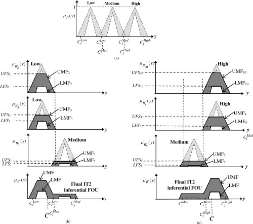
An evolutionary optimization realized with DE is used here for optimal setting of class boundaries (along with ) satisfying the above criteria. The structure of the IT2FS used for the 3 classes are shown in Fig.4 (a) for convenience.
The ~ (y)
j B
is constructed with the centre of its base located at ( Y Y) / 2
l r
C C and is symmetric around the
vertical axis passing through the centre. The UMF of the consequent IT2FS is considered normal (i.e., the peak membership = 1). The LMF of the consequent IT2FS is constructed as a relatively smaller isosceles
Fig. 4 (a). Consequent IT2 MF for 3 classes: Low, Med. and High cognitive loads with initial class centroid positions , (b) defuzzified output C falls in Low cognitive load class after firing of rule 2, 3 and 7, (c) defuzzified output C falls in High cognitive load class after firing of rule 10, 8 and 5.
Low Medium
y y Med l C 1 Low Low Medium Final IT2 inferential FOU y ) (y B ) ( 7 y B ) ( 3 y B ) ( 2 y B y y y C High High Medium Final IT2 inferential FOU C ) (y B ) ( 5 y B ) ( 10 y B ) ( 8 y B ) (y B y Low l
C CrLow CrMed ClHigh
(a)
(b) (c)
UMF2 LMF2 UMF3 LMF3 UMF7 LMF7 UMF8 LMF8 UMF10 UMF5 LMF5 UMF
LMF UMF
LMF y y Low l C Med r C Med l
C ClHigh
triangle with intuitively chosen base-width = 40% of the base-width of the UMF and height = 80% of the height of the UMF. This in other words offers a large tolerance to Y
l
C and CYr to improve classification
accuracy.
Let x1x1,x2 x2,..,xmxm be a measurement point. We obtain the lower firing strength (LFSj) and
upper firing strength (UFSj) at the measurement point for rule j by (12) and (13).
))) ( ( , ( , ~
1 A k
m
k j
j Min w Min x
LFS
k j
(12)
))) ( ( , ( , ~
1 A k
m
k j
j Max w Min x
UFS
k j
(13)
Here, wjand wj, lying in [0, 1], are respectively the upper limit of
, 1
( ( ))
m
k A j k k
Min x
and lower limit of
, 1
( ( )).
m
k A j k k
Min x
The introduction of the wjand wjin (12) and (13) provides a mechanism to control the area
under the consequent FOU, thereby controlling the location of the centroid of the resulting consequent IT2 MF. The optimal values of wjand wjare determined by an evolutionary algorithm with an aim to maximize
the classification accuracy for individual classes. Although any evolutionary algorithm could serve the purpose, we selected the well-known DE algorithm [49] for its simplicity in coding, fewer control parameters and above all our familiarity with the algorithm [32]. The optimal selection of wjand wjis
undertaken in the experiment section.
We now compute the consequent IT2 MF ( )
j
B y
with UMF and LMF obtained by (14) and (15).
( ) ( ( )), )
j j j
B y Min B y UFS
(14)
( ) ( ( )), )
j j j
B y Min B y LFS
(15) In case more than one rule with same or different class labels at the consequent are fired by instantiation of the antecedent linguistic variables, then we obtain the final inference Bby taking union of the individual inference Bj, for all j.
j j B B
= [ j
j B j j B ] (16) Here, B refers to an IT2FS, whose LMF and UMF are the maximum of the constituent Bjs’ LMF and UMF respectively. We next obtain the left and the right end point centroids Cl and Cr respectively of the
resulting IT2MF Bby using the well-known Karnik Mendel (KM) Algorithm [31], and hence determine the centroid C of the resulting IT2Fs using (17). The centroid C here represents the cognitive load of the subject. 2 r l C C
C (17)
The KM algorithm aims at finding the left (right) switch point from the UMF (LMF) to the LMF (UMF) in an iterative manner, such that the centroid of one embedded fuzzy set, following the UMF (LMF) up to the switch point and following the LMF (UMF) after the switch point, is equal to the switch point. The left (right) end switch point is defined as left (right) end point centroid.
Lastly we determine the class Y of the input measurement by determining the class interval [CYl CrY], that
In Fig. 4, we schematically demonstrate the computation of Bfrom B~jfor all j, and next show results of
computation of Cl and Cr and the centroid C of B for firing of 2 sets of rules. For the first set of rules, the
centroid C is found to lie in [ Low Low],
l r
C C whereas for the latter set of rules, the centroid falls in [ High High],
r l
C C
indicating Low and High classes as the resulting classifier outputs in Fig. 4(b) and (c) respectively.
C.GT2FS Induced Classifier Design
A GT2FS [35] is a three tuplex,u (x),μ(x,u)
A~ , where x is a linguistic variable (here, feature value), u~A(x) is
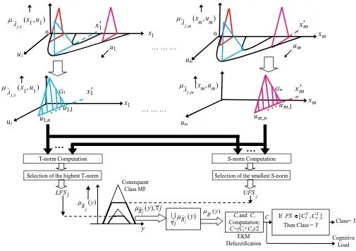
the primary MF and (x,u)is the secondary MF. Both the primary and the secondary MFs lie in [0, 1]. Here, we present a GT2FS in vertical slice form [35] (Fig. 5), where each vertical slice represents secondary MF with respect to primary membership at a given xx, say. Given a GT2FS classifier rule j: If x1 is A j,1, x2 is
,2
A j , ..., xm isA~j,mThen class centroid y of ~ (y)
j B
lies in [CYl CrY]. Here, xk is Aj,k ~
for k = 1 to m are GT2FS-induced propositions and ~ (y)
j B
denotes an IT2FS consequent MF.
Definition 1: We define the t-norm (denoted by X t
) between two vertical planes ( , )
) ( ,
~ pl
p x p j A p u G
and
) ( ,
) ( ,
~ qv
q x q j A q u G
of A~j,p and A~j,q respectively by (18).
]}. , 1 [ , | ) ( t ) ( { X , ) ( , ~ , ) ( ,
~ u u lv n
G
G qv
q x q j A l p p x p j A q t
p (18)
Here, we take t = min. For any three vertical planes Gp, Gq and Gr taken from A~j,p, Aj q, and Aj r, , the
cumulative t- norm is defined by
X X ( X ) X .
t t t t
p q r p q r
G G G G G G In general, the cumulative t-norms of G1, G2, … , Gm, taken from m distinct
GT2FS, is evaluated in the fixed order of occurrence of Gk, k = 1 to m. Fig. 5. Secondary Membership Assignment
) ( ) ( ~ 2 ,
, x i
Aji i u
) ( ) ( ~ 1 ,
, x i
Aji i u
,1 i u
..
. . . ui,2n i u, i x 2 , i
x xi,3 1 , i x 1 ) , ( ,
~ i i
Aji x u
i u 0 ) ( ) ( ~ 2 ,
, x i
Aji i u
Definition 2: To compute the s-norm between two vertical slices Gp and Gq introduced above, we simply
replace t by s in (18), where we take s = max. The cumulative s-norm is computed by replacing t by s (=max) in cumulative t-norm.
Given a measurement point: xk xk for k = 1 to m, we obtain the firing strength of rule j by the following
five steps (Fig. 6).
1.Let ( 1,)
) 1 ( 1 , ~ 1 u G x j A
, ( 2)
) 2 ( 2 , ~ 2 u G x j A
,…, Gm = ( ,).
) ( , ~ m m x m j
A u
We computeGGtG t...tGm 2
1 by (18) to obtain m
n terms in G.
2.We evaluate the largest of the nm terms in G and call it ,
j LFS i.e., )} ( ... ) ( ) ( { ) ( , ~ 2 ) 2 ( 2 , ~ 1 ) 1 ( 1 , ~ m m x m j A x j A x j A
j Max u t u t t u
LFS (19) 3.Similarly we compute 1 2 ... .
s s s
m
H G G G
4.We evaluate the smallest of the nm terms in H and call it ,
j UFS i.e., )} ( ... ) ( ) ( { ) ( , ~ 2 ) 2 ( 2 , ~ 1 ) 1 ( 1 , ~ m m x m j A x j A x j A
j Min u s u s s u
UFS (20) Fig. 6. GT2FS Classifier Design
… … … … … … … .. um m x m x m u ) , ( ,
~ m m
Ajm x u
0
…
1 x 1 x ) , ( 1 1 ~ 1 , u x j A 0 u1 1 u
.
j LFS…
Consequent Class MF ) ( ~ y j B ) ( ~ y B ( ) j B j y EKM Defuzzification
Cl and Cr Computation;
C=(Cl+Cr)/2
( ),
j
B y j
u1 1 x 1 , 1 u
.
.
nu1,
. . ) , ( 1 1 ~ 1 , u x j A 1 x . G1 j UFS m x m x 1 , m u
.
.
.
n m u , . . . ) , ( ,~ m m
Ajm x u
um
Gm
y
T-norm Computation
Selection of the highest T-norm
S-norm Computation
Selection of the smallest S-norm
C If FS[ClY,CrY]
Then Class = Y Class= Y
It can be easily verified that UFSj ≥ LFSj. Further, UFSj and LFSj provide the Least Upper bound (LUB)
and the Greatest Lower Bound (GLB) of the constituent secondary MFs, each contributed by one vertical plane of m antecedent GT2FS.
5. Compute the consequent IT2 MF ( )
j
B y
with UMF and LMF obtained by (14) and (15).
6.If multiple rules fire for Bj, then we need to take the union of all the type-2 inferences as indicated in (16).
7.Next we decode (defuzzify) the type-2 inference class using EKM Defuzzification technique [30] and obtain left and right end point centroids Cl and Cr. We finally evaluate the class centroid C by (17).
Now, identify the pre-defined class by defining the class interval [ClY CYr],that includes the class centroid C.
If C falls in the above interval, then class = Y.
IV. EXPERIMENTS AND RESULTS
A. Experimental Set-up
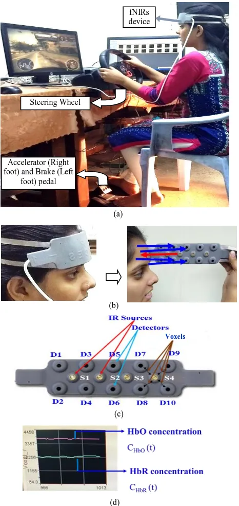
Experiments are undertaken with a Logitech driving simulator, comprising one steering wheel, one brake and one accelerator foot pedal and a monitor to drive the simulated car (Fig. 7(a)) and an fNIRs device, manufactured by BIOPAC, with 4 infrared (IR) sources and 10 infrared detectors, placed in an array for mounting on the forehead (Fig. 7(b)). The IR sources are triggered by short duration electrical pulses in a time-multiplexed manner to ensure activation of only one source at a time. On triggering of a selected source, the infrared signal penetrates the pre-frontal region below the source, and the received energy is partially absorbed by the brain and partially reflected back to the four detectors mounted around each source (Fig. 7(c)). The sampling rate of the fNIRs device being 2 Hz, the sampling intervals are of 0.5 seconds. The sampling interval constitutes four equal time-slices of 0.125 seconds, where each time-slice is utilized to receive oxygenated (HbO) and deoxygenated (HbR) blood response (Fig. 7(d)) by one of four detectors around each source. Thus for 4 sources, we obtain 16 oxygenated and 16 deoxygenated blood response of 16 voxels (brain regions) in 0.5 seconds. It is important to note that the penetration depth of the IR signals is 1.25 cm from the surface of the scalp. The signal acquisition is performed using (Cognitive Optical Brain Imaging)COBI studio software, supplied by the manufacturer.
B. Participants
Forty right-handed volunteers (driving learners), in the age group: 20-55 years with normal/corrected vision participated in this experiment. The participants include 37 healthy subjects (20 male and 17 female) and 3 male patients suffering from the Alzheimer’s disease.
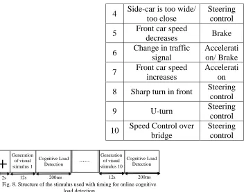
C. Stimulus Presentation for online classification
TABLE I
LIST OF STIMULI AND REQUIRED ACTIONS
S. No .
Type of stimulus Required
action
1 Making Right Turn Steering Right 2 Making Left Turn Steering
Left 3 Bumper ahead Brake (c)
Voxels
(b)
(d)
Fig. 7 (a) Experimental set-up with fNIRs data acquisition (b) IR penetration into the brain and its detection by the fNIRs
device, (c) Structure of the fNIRs device (d) HbO and HbR concentration plot of a voxel
Accelerator (Right foot) and Brake (Left
foot) pedal Steering Wheel
fNIRs device
4 Side-car is too wide/ too close
Steering control 5 Front car speed
decreases Brake 6 Change in traffic
signal
Accelerati on/ Brake 7 Front car speed
increases
Accelerati on 8 Sharp turn in front Steering
control
9 U-turn Steering
control 10 Speed Control over
bridge
Steering control
D. Experiment 1: Demonstration of decreasing Cognitive Load with increasing Learning Epochs for
similar stimulus
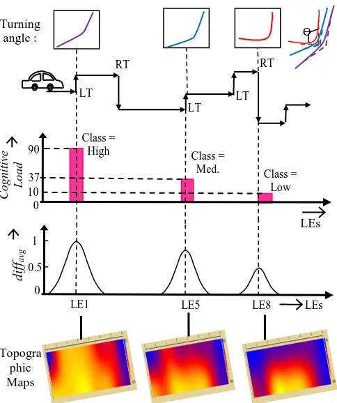
The motivation of the present experiment is to estimate the cognitive load in motor-learning from the prefrontal activation. We here estimate and classify the cognitive load in 3 classes. It is noted that with increased learning epochs the cognitive load is decreasing. The same observation also follows from the measure of diffavg and also the topographic maps produced by the COBI studio software [41].
The above estimation is carried out over different learning epochs (LEs) for each of the 10 stimuli indicated above. Fig. 9 provides the diffavg, the topographic maps and cognitive load classes obtained in
three different LEs of making right and left turns (stimuli 1 and 2). Here, we confirm that the subject is able to learn to take left/right turns (LT/RT) efficiently from the gradual decrease in turning-angle Ɵ. Simultaneously, the peak of the diffavgalong with computed cognitive load falls off gradually with repeated
left/right turning and/or LEs. It is apparent from Fig. 9 that the first trial of learning incurs high cognitive load (symbolized in yellow), whereas the fifth trial for the same motor task yields medium cognitive load (symbolized in red). Lastly, the lowest activity (marked in blue) appears in the eighth trial of learning
+
Generation of visual stimulus 12s
Cognitive Load Detection
Generation of visual stimulus 10
Cognitive Load Detection
12s 200ms 12s 200ms
... ..
resulting in low cognitive load. The decrease in cognitive load with increased learning epochs that follows up from this experiment is also supported by existing works [44].
E. Experiment 2: Automatic Extraction of discriminating fNIRs Features
We adopt two approaches for feature selection. First we obtain the 8 features out of 480 with an aim to maximize inter-class separation and minimize intra-class separation, which is done by minimizing (5). A cross-check of these 8 optimal features is also evident from the feature value plot (Fig. 10) for three classes. It is clear from the plot that the features F51 (Mean HbO conc. of voxel 3), F120 (Mean HbO conc. of voxel 6), F123 (Mean HbO conc. of voxel 8), F207 (Mean HbO conc. of voxel 16), F300 (avg. energy of voxel 5), F372 (avg. energy of voxel 12), F417 (avg. slope of voxel 5) and F471 (skewness of voxel 14) offer maximal inter-class separation.
F. Experiment 3: Optimal Parameter Setting of Feature Selection and Classifier Units
Here, we use 2 DE-based optimizers, working in double loops. The inner loop is maintained by the left-cornered DE in Fig. 11, whereas the outer loop is maintained by the central DE. The left left-cornered DE is used to select the optimal features by minimizing (5) with a given value of produced by the right DE
No
rm
ali
ze
d
F
ea
tu
re
Va
lu
es
Static and dynamic Features Fig. 10. Extracted fNIRs features to discriminate cognitive load of 3 classes.
(The eight features, shown by the dotted line are most discriminating)
F51 F120 F123 F207 F300 F372 F417 F471
Fig. 9. The cognitive load, diffavg and the topographic maps obtained during the learning phase of left/right turning
LT RT
LT RT
Turning angle :
LT
Ɵ
LE5 LE8 LEs
d
iffavg
LE1
Topogra phic Maps
1
0 0.5
Co
g
n
it
ive
L
o
a
d
90
37 10 0
LEs
Class =
High Class =
optimizer, used for parameter selection. For a given ,the left cornered DE on convergence produces the
(tentative) best 8 out of 480 features by minimizing (5). These features are used by the GT2FS/IT2FS classifier for initializing the classifier parameters to produce class iY. The DE-based parameter selection then attempts to minimize
, ) ( 2
i
i a i
Y Y
J (21)
subject to
. 100 and
0
, ,
, 5 . 0 001 . 0
. .
High r High l
Low r Low l
High l Med r
Med l Low r
C C
C C
C C
C C
(22)
Here, a i
Y = actual class label of the i-the training instance and
Fig. 11. Parameter selection of the GT2FS classifier for each healthy subject’s 81 data-points of 480 dimensions
The process explained above is repeated until both the DEs converge. Once converged, the η and classifier parameters ( , , ., ., lHighand rHigh)
Med r Med l Low r Low
l C C C C C
C are selected for online feature selection and classification.
This is schematically illustrated in Fig. 11. The optimal parameters of GT2FS classifier and are obtained as follows.
= 0.0028,
Low l
C =7.16, CrLow ClMed.24.22, . 62.28
High l Med
r C
C
and High r
C =98.6.
In Fig. 12, we do the same for the IT2FS classifier. Here, we need to optimize wjandwjalong with other
classifier parameters (ClLow,CrLow,ClMed.,CrMed.,ClHighandCrHigh)and η. Here, we attempt to optimize (21),
subject to
0wjwj1,
other classifier parameter constraints, and constraints on η, given in (22).
Fig. 12 explains the mechanism of the parameter selection for the IT2FS classifier and feature selection unit. After the parameters are obtained, we go for online classification of unknown input instances to classify the cognitive load into three classes: Low, Med. and High. The optimal values for the parameters of IT2FS classifier are listed below:
= 0.00281,
Low l
C = 7.72, CrLowClMed.24.01, CrMed.ClHigh 62.63
and High r
C = 98.12,
, 86 . 0
1
w w10.20, w20.78, w20.12, w30.84, w30.12, w40.68, w40.42,w50.78, w50.32, w60.91, w60.18, ,
84 . 0
7
w w70.23, w80.97, w80.20, w90.86, w90.22,
10 0.90
w and w100.12.
V.BIOLOGICAL IMPLICATIONS
The cognitive load distribution in prefrontal cortex (PFC) over the LEs is presented here by a voxel plot using MATLAB 2016 version. The mean of CARα(t) for α = 1 to 16 voxels are plotted as a 2 × 8 voxel plot
demonstrating the 16 channels of the fNIRs system as shown in Fig. 13. The voxel plots indicate that 37 healthy subjects yield similar behavior in the activation pattern of PFC, irrespective of their age and gender. However, reduced dorsolateral PFC (DLPFC) activation associated with low learning ability is possibly related to improper growth/partial damage of the brain lobes [48], which we noticed in three Alzheimer’s patients.
The following biological implications directly follow from the voxel plot of Fig. 13.
1. The left PFC has relatively higher activation than the right PFC when the subject experiences cognitive load in motor learning stimuli.
2.Fig. 13, depicting the regional response of the PFC, demonstrates that cognitive load shifts from the orbitofrontal cortex (OFC) to the ventro-lateral PFC (VLPFC) with increased LEs for healthy subjects. The brain anatomy responsible for OFC activation is associated with Broadmann area 11 (BA11), which has a significant involvement in reasoning, complex decision making, planning, and encoding new information into memory [45]-[47].
3.A significant reduction in the DLPFC activation is observed when cognitive load shifts from High to Low for the healthy subjects.
The graph shown in Fig. 14 also indicates that the cognitive load value (CLV) has a similar behavior with OFC activation for 3 different cognitive loads for the healthy subjects. The rest of the graphs are apparent and thus need no explanation.
VI. PERFORMANCE ANALYSIS
This section provides experimental basis for performance analysis and comparison of the proposed classifiers with traditional/existing ones.
A. Performance Analysis of the proposed IT2FS and GT2FS classifier
To study the relative performance, we undertake three levels of analysis: i) classification accuracy, ii) run-time complexity of the classifiers and ii) joint occurrence of true (T)/false (F) and positive (P)/negative (N) cases. Table II contains the mean percentage classification accuracies of the proposed type-2 fuzzy classifiers against traditional fuzzy and non-fuzzy ones, including two existing GT2FS models [1] and [37], four existing IT2FS models [1], [50]-[52], evolving Type-2 Fuzzy Classifier (eT2Class) [29], Type-1 Fuzzy Neural Network [57], traditional type-1 Fuzzy set, SVM-RBF, LSVM, Linear Discriminant Analysis (LDA) [54] and k-Nearest Neighbor (kNN) [53]. In Table II, the percentage accuracy of each classifier is evaluated using (22), where TP, TN, FP and FN are the numbers of true positives, true negatives, false positives and false negatives respectively [37].
Fig.14. CLV variations in the prefrontal lobe with decreasing cognitive load
C LV
CLV DLPFC
VLPFC OFC
100
50
0
High Med. Low
Scale Factor - CLV: Scale: 1 DLPFC
VLPFC Scale: 5 OFC
OFC
DLPFC DLPFC
VLPFC BA11 VLPFC
(a) (b)
(c) (d)
20
0
Fig.13 (a) Regions of the PFC; Voxel plot of the fNIRs data at (b) LE4 (Cognitive load: High), (c) LE10 (Cognitive Load: Med.) and (d) LE15
FN FP TN TP TN TP Accuracy Classifier
(22)
The experiment is accomplished with 11340 training instances for 37 healthy subjects and 3 brain-diseased subjects. Table II indicates that the proposed IT2FS and GT2FS classifiers outperform their nearest competitors by an average classification accuracy of ~ 1% and ~2% respectively.
TABLE II
MEAN PERCENTAGE CLASSIFICATION ACCURACY (STANDARD DEVIATION) OF PROPOSED CLASSIFIERS AGAINST STANDARD CLASSIFIERS FOR COGNITIVE LOAD DETECTION OF DRIVING LEARNERS
Classifier s No. of free parame ters Mean classifier accuracy in % (standard deviation) HIG
H
MED
. LOW
Proposed
GT2FS 7
97.76 (0.03 11) 95.94 (0.01 23) 96.29 (0.0113) Proposed
IT2FS 27
96.29 (0.01 04) 94.93 (0.00 12) 95.23 (0.0127) SA-GT2FGG [37] 17 88.10 (0.01 67) 85.14 (0.02 31) 88.91 (0.1239)
GT2FS-NN [1] 1
93.16 (0.09 21) 90.16 (0.02 13) 91.26 (0.0134) eT2Class
[29] 33
94.12 (0.01 21) 91.12 (0.01 01) 93.12 (0.0211) IT2FS-NN
[1] 10
96.12 (0.01 01) 94.16 (0.02 16) 93.13 (0.0114) McIT2FIS
[50] 210
93.42 (0.01 46) 90.89 (0.02 15) 91.34 (0.0121) ST2FNN
[51] 172
Classifier
SVM-RBF 4
92.31 (0.02
15)
91.19 (0.02
91)
92.14 (0.0216)
LSVM 3
89.25 (0.02
19)
86.93 (0.02
14)
87.19 (0.0198)
LDA 3
89.72 (0.02
11)
87.00 (0.02
11)
80.11 (0.0181)
kNN 2
91.12 (0.02
17)
90.11 (0.02
01)
92.13 (0.0215)
Table III contains the times of the proposed type-2 classifiers against the traditional ones. The run-time complexity analysis of table III shows that our proposed IT2FS classifier algorithm requires the smallest run- time (~34 milliseconds) among all the classifiers and the proposed GT2FS classifier takes 94.23 milliseconds, which is also comparable to the run-time of the existing IT2FS classifiers, proposed in [50], [52].
TABLE III
RUN-TIME OF THE PROPOSED CLASSIFIERS AND OTHER COMPETITIVE CLASSIFIERS
Classifiers
Run-time in HP Dual-core
machine
Proposed GT2FS 94.23 ms
Proposed IT2FS 33.72 ms
SA-GT2FGG [37] 98.18 ms GT2FS-NN [1] 96.12 ms eT2Class [29] 45.15 ms IT2FS-NN [1] 38.22 ms McIT2FIS [50] 95.18 ms ST2FNN [51] 92.00 ms McIT2NFIS-RBE [52] 100.4 ms
Type 2 Fuzzy Set
induced Classifier [22] 48.94 ms Type 1 Fuzzy Set
induced Classifier 51.42 ms
SVM-RBF 40.12 ms
LSVM 35.98 ms
LDA 48.25 ms
kNN 35.11 ms
Finally, the relative performance of all the type-2 fuzzy classifiers, listed in Table IV, is compared by considering the 2 distinct classifier performance metrics: True Positive rate (TPR), and True Negative Rate (TNR) [37], given by (23) and (24). Here, GT2FS is found to outperform all existing and the proposed IT2FS classifier algorithm by around 1-3% of TPR value.
% 100
FN TP
TP
% 100
FN TP
TN
TNR (24)
TABLE IV
COMPARATIVE STUDY OF PERCENTAGE TPR AND TNR OF THE PROPOSED CLASSIFIERS WITH EXISTING GT2FS AND IT2FS CLASSIFIERS
Classifier Performance Metrics
TPR% TNR%
GT2FS
(proposed) 98 96
IT2FS (proposed) 97 95
SA-GT2FGG [37] 89 87
GT2FS-NN [1] 91.13 87.24 IT2FS-NN [1] 89.87 84.15 McIT2FS [50] 92.82 1.88
ST2FNN [51] 92.13 90.97 McIT2NFIS-RBE
[52] 77.79 72.98
B. Statistical Validation of the classifier using McNemar’s Test
We select McNemar’s test [36] to compare the relative performance of the proposed DE-based feature selection induced GT2FS classifier with the other standard classifiers (Table VI). The statistical validation is performed with only one database prepared at Brain Imaging Laboratory of Jadavpur University. Most of the statistical tests [68] undertaken to compare classifier-performance require a large number of databases to determine the z-score metric used to accept/reject the null hypothesis (that all classifiers are equally good). Unfortunately, for the present experiment we prepared a single database, and so we use the McNemar’s test, which requires a single database for statistical validation of the classifiers [36].
In Table V, Z indicates the probability of accepting/rejecting the null hypothesis, which indicates that all the classifiers are equally good. Table V confirms that the proposed GT2FS classifier is comparable with the proposed IT2FS classifier only.
TABLE V
STATISTICAL VALIDATION OF THE CLASSIFIERS USING MCNAMER'S TEST
Reference Algorithm: Proposed GT2FS Induced Classifier
Classifier algorithm used for comparison using the 20
optimal features
Parameter s used for McNemar
’s Test Z
Comments on acceptance
/ rejection
of hypothesis
m n
Proposed
IT2FS 5 14
3.68
4 Accept
SA-GT2FGG
[37] 20 49
11.3
6 Reject GT2FS-NN [1] 12 57 28.0
eT2Class [29] 13 36 9.87
7 Reject IT2FS-NN [1] 22 45 7.22
3 Reject McIT2FS [50] 7 18 4.O
O Reject ST2FNN [51] 16 33 5.22
4 Reject
McIT2NFIS-RBE [52] 18 35 4.83 Reject Type 2 Fuzzy
Set induced Classifier
20 65 10.1
2 Reject Type 1 Fuzzy
Set induced Classifier
29 73 18.1
3 Reject SVM-RBF 22 39 4.19
7 Reject
LSVM 15 33 6.02
1 Reject
LDA 17 67 28.5
8 Reject
kNN 19 39 6.22
4 Reject
VII. CONCLUSIONS
The paper proposes a novel approach to cognitive load assessment and classification of driving learners using an fNIRs device. A GT2FS induced classifier has been developed and tested over 37 healthy subjects and 3 brain patients using a laboratory model of a driving set-up. Experiments undertaken reveal that the proposed classifier outperforms its competitors by a large margin. A statistical test undertaken confirms the better classifying ability of the proposed GT2FS classifier over its competitors. The proposed system would have applications to identify people with high cognitive load for moderate/low traffic conditions, thereby saving people from having a psychological set-back/trauma due to tremendous mental pressure in high cognitive load. Biological implication of the research results is also narrated briefly here. It is apparent from the voxel plots that DLPFC and OFC are primarily engaged in HIGH cognitive load tasks. They are less influenced when the cognitive load is reduced. Determining the cognitive pathways in the brain during the learning phase of driving is another interesting and open problem. A detailed study of this using fNIRs alone is almost next to impossible. One approach to solve it perhaps is to compositely utilize both cortical signals by EEG or otherwise along with brain activation results obtained from fMRI and/or fNIRs devices. Acknowledgment
The authors gratefully acknowledge the funding they received from the UPE-II Project in Cognitive Science offered by University Grants Commission (UGC) to Jadavpur University.
REFERENCES
[1] A. Saha, A. Konar, and A. K. Nagar, "EEG Analysis for Cognitive Failure Detection in Driving Using Type-2 Fuzzy Classifiers." IEEE Trans. Emerging Topics in Computational Intelligence pp: 437-453, 2017.