Iran. J. Chem. Chem. Eng. Vol. 27, No. 4, 2008
A New Method for Time-Delay Compensation
in Control Systems
Shirvani, Mansoor*+; Esmaeli, Mansooreh
Department of Chemical Engineering, Iran University of Science and Technology, P.O. Box 16846-13114 Tehran, I.R. IRAN
ABSCTRACT: In this paper a new method is introduced and investigated for removing the destabilizing effects of time-delay parameter in control loops. The concept of the method is taken from the knowledge concerning the dynamic behaviour of irrational transfer functions (Ir-TF), which is discussed and investigated elswhere in frequency response domain and is explained briefly here. Ir-TFs, which are well capable of representing the model structure of a wide range of distributed parameter process systems are known o have transcendental characteristics in their frequencyresponses.The main complexity of these systems is in their phase behavior, which appears to have the capability torepresent acomplete time-delaycharacteristic as well as the characteristics in which the effect of time-delay is much limited. The conditions for appearance of the above dual phase characteristics may guide one to synthesise a contol loop in which the non-minimum phase dinamics of the open-loop transfer function is removed. This concept, when used in a simple loop by using a suitable predictor, affects the robustness features of the loop in a desirable manner and improves the stability characteristics of the loop, provided that the required conditions for the predictor is established. In addition to the important robustness property, the proposed time-delay compensator provides some advantages and specific properties in comparison to the conventional Smith predictor. These are the capability to be used for controlling the processes with an irrational transfer function model as well as the integrated processes that include time-delay parameter.
KEY WORDS: Irrational transfer function, Time-delay compensation, Phase limitter, Non-minimum phase, Dominant gain.
INTRODUCTION
Time-delay, in control systems, is an important problem due to the destabilizing effects and the corresponding sluggishness in the loop response. It introduces into the control loops either by measurement and the final control element or by the process system
itself as an inherent parameter of the system. It is notable also thatexceptionallargeamountof time-delay parameter in process systems is not rare. Examples are the rotary drum systems and the heat exchangers and etc. The Smith predictor, shown in Fig. 1, is the first attempt in the
*To whom correspondence should be addressed.
+E-mail: [email protected]
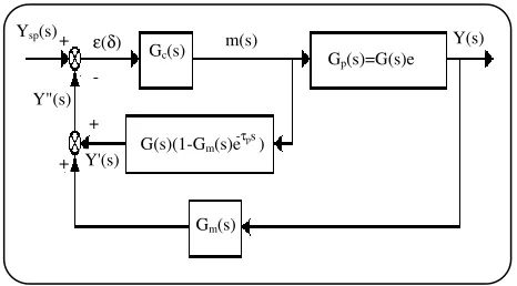
Fig. 1: Smith predictor control loop.
literature for removing the destabilizing effects of time-delay in control loops [1]. In this method the attempt is to remove the time-delay parameter effect from the open loop transfer function or from the input signal to the controller.
In this figure Gp(s) is the transfer function of the process, which is composed of the non-delay part, G(s),
and the delay part e−τds. Also, Gc(s) is the controller and Gm(s) is the measuring element. Later, it was revealed that Smith's method which is based on omitting the true value of time-delay parameter from open loop transfer function, suffers from some important problems such as severe sensitivity to model mismatches [2,3], as well as lack of capability to remove offset from the loop response in disturbance rejection, when dealing with time-delay included integral processes [4-6]. Numerous modified time-delay compensations (DTCs) had appeared in the literature [4-13]. The largest deficit of DTC-based methods is lack of application for process models in which the time-delay can not be factored out straight from the transfer function and their transfer function are irrational. In [14], for solving this problem, under the inspiration of smith’s method, irrational transfer function
(Ir-TF) model is divided into two parts: Gp+(s), part of
the model that includes Right Half Plane (RHP) zeros,
and Gp−(s), part of the model that does not include RHP
zeros. By removing the effect of Gp+(s) from the open loop transfer function and input signal to the controller, the behavior of control system is changed from non-minimum phase to non-minimum phase. In this method [15] has been used for flow control. However, it is notable that the estimation of RHP zeros is difficult and inaccurate since it is solved numerically.
In this paper a new method is proposed for limiting the non-minimum phase dynamics of the time-delay parameter in the control loop, such that the effects of right half plane zeros (without requiring to compute them) as well as the high order effects in the loop, also, are removed simultaneously. This method is based on the basis of a special characteristic which is investigated and revealed to be existent in the dynamic behavior of Ir-TF models. This characteristic, after being discussed, was used to introduce a predictive signal to the controller for the purpose of limiting the time-delay effect in the open loop transfer function or the input signal to the controller. Thus, the control scheme was named model bypass phase limiting-predictive (MBPL-predictive) control.
DYNAMIC BEHAVIOR OF IR-TF
The concept of irrational transfer function (Ir-TF) and its dynamic behavior is the essence of the method which is used in this paper for decreasing destabilizing effects of time-delay in control loops. Dynamic behaviors of Ir-TFs have been investigated in frequency response domain [14, 17-19]. An Ir-TF model which is considered here composes of parallel combination of two rational transfer function elements.
s T 2 1 2
1(s) G (s) G (s) G (s)e d
G ) s (
G = + = + ′ − (1)
(
)
(
)
(
)
(
)
s T L
1 l
l , m p
J 1 j
j , n 2 K
1 k
k , m p
I 1 i
i , n 1
d
2 2
1 1
e 1 s s
1 s K
1 s s
1 s K
−
= =
= =
∏
∏
∏
∏
+ τ
+ τ
+ + τ
+ τ =
Where, I≤K and J≤L, and p=-1,0,1 represents the existence or not existence of a pole or zero at the origin of the complex plane.
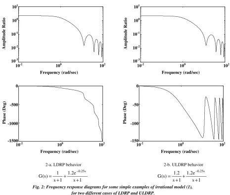
One of the elements of the model includes time-delay parameter, while the other is a delay free rational transfer function. A unique feature of the dynamic behavior of this model structure is the resonating characteristic, appearing in its frequency response, both in gain and phase of the model. The main complexity in the dynamics of such models is the dual behavior of the model regarding the effectsof time-delayparameterinthe model, [14]. Depending on the amount of the parameters of the model its dynamic behavior can be divided into two major categories. One is named here as the limited-delay-resonating-phase behavior (LDRP behavior), andthe other Gp(s)=G(s)e
G(s)(1-Gm(s)e ) -τps
Gm(s) Gc(s)
ε(δ) m(s)
Y"(s)
Y'(s)
Y(s) +
Ysp(s)
+
Iran. J. Chem. Chem. Eng. A New Method for Time-Delay … Vol. 27, No. 4, 2008
2-a. LDRP behavior 2-b. ULDRP behavior
1 s e 2 . 1 1 s
1 ) s ( G
s 25 . 0
+ + + =
−
1 s e 2 . 1 1 s
2 . 1 ) s ( G
s 25 . 0
+ + + =
−
Fig. 2: Frequency response diagrams for some simple examples of irrational model (1), for two different cases of LDRP and ULDRP.
one is the unlimited-delay-resonating-phase behavior (ULDRP behavior). In the LDRP behavior the model demonstrates a resonating characteristic in its phase around a limited average value at high frequencies, while in the ULDRP behavior there is no high frequency approach to a limiting value in the phase diagram. These twocases are demonstrated in Fig. 2 for some simple, low order rational functions G1(s) and G2(s). It is interesting to note that only by changing the position of time-delay (or the position of gains of the elements in the model) in this figure, the behavior of the phase of the model is completely changed, while that of gain is remained unchanged. However, the behavior shown in Fig. 2-b, is much desirable than that of 2-a, from the control point of view.
In case of appearing LDRP behavior in the phase of the model, vector G(jω) traces the gain and phase of
G1(jω), which is a delay free rational model, while in the ULDRP behavior the model traces the gain and phase of G2(jω), which includes delay parameter. The above dual characteristic is well recognizable in a heuristic manner by tracing the Nyquist plot of the model as well as its individual elements in comparison. The original concept which can be used for detecting the origin of appearance of the above dual behavior of the phase is demonstrated in Fig. 3 [16-18]. It is also investigated by [14], with respect to the existence of right half plane zeros in the irrational models in (1).
In Fig. 3, the positions of the vectors G1(jω) and G2(jω) are shown in comparison at an specific ω, where the two vectors stay in opposite direction relative to each other. Due to the existence of time-delay parameter in vector G2(jω), this vector is supposed to be faster in rotation than G1(jω). Concerning the LDRP behavior,
101
100
10-1
10-2
10-3
A
m
p
li
tu
d
e
R
at
io
10-2 100 102 Frequency (rad/sec)
101
100
10-1
10-2
10-3
A
m
p
li
tu
d
e
R
at
io
10-2 100 102 Frequency (rad/sec)
0
-500
-1000
-1500
P
h
as
e
(D
eg)
10-2 100 102 Frequency (rad/sec)
0
-50
-100
-150
P
h
as
e
(D
eg)
Fig. 3-b depicts the relative position of |G2(jω)| and |G2(jω)| in polar plot, where |G1(jω)|>| G2(jω)|. Therefore, in this condition, the Nyquist plot of the model traces the Nyquist plot of the element G1(jω). If G1(jω) does not encircle the origin of the complex plane, the resulting Nyquist plot of the model does not encircle the origin, as if the time-delay is not present in the model. Contrary to Fig. 3-b, in Fig. 3-a, which is corresponding to the ULDRP, |G1(jω)|<|G2(jω)|, and the resulting gain of the model encircles the origin of the complex plane, while tracing the niquist plot of G2(jω), the delay included element of the irrational model. A detailed tracing of the Nyquist plots of the model and its elements declares the periodic resonances appearing in the gain and phase of G(jω), as well as the above origin encircling and non-encircling characteristics in the complex plane.
Fig. 4 demonstrates a full tracing of the Nyquist plots for an irrational model in which the element G2(jω) contains a time-delay parameter and |G1(jω)|>|G2(jω)|. Thus the irrational model, G(jω), traces and resonates around the Nyquist plot of G1(jω), which does not encircle the origin and approaches a finite value of phase as ω approaches infinity. In Fig. 5 the opposite situation is created by interchanging the gains of the elements of the model by each other. Thus, the G(jω) encircles the origin, while tracing the Nyquist plot of G2(jω).
The final conclusion of the above statements is that in the irrational model of (1) the gain and phase of the model traces and resonates around the gain and phase of one of the elements of the model. This element will obviously be the dominant gain one. Therefore, if for instance, the dominant gain element is a first order transfer function without time-delay, then all of the non-minimum phase effects included in the other element of the model will be collected and recovered by the dominant gain one. A proof of this statement is presented in appendix A. Thus, it would be possible to change the behavior of the model from ULDRP to LDRP by adjusting the parameters of the elements of the model relative to each other such that the condition; |G1(jω)|>|G2(jω)|, ∀ω establishes.
MODEL- BYPASS-PHASE- LIMITER-PREDICTOR (MBPL-Predictor)
The above concept of changing the phase behavior of an Ir-TF model, simply by adjusting the amounts of
(a) - "ULDRP behavior" (b) - "LDRP behavior"
Fig. 3: Detecting the origin of appearance of dual phase behaviors in frequency response of Ir-TF models.
Fig. 4: The Nyquist plot of G(jωωωω)= G1(jωωωω)+ G2(jωωωω) traces the Nyquist plot of G1(jωωωω) in a resonating behavior, where |G1(jωωωω)|>|G2(jωωωω)|; ∀∀ω∀∀ωωω.
Fig. 5: The Nyquist plot of G(jωωωω)= G1(jωωωω)+ G2(jωωωω) traces the Nyquist plot of G2(jωωωω) in a resonating behavior,where |G1(jωωωω)|<|G2(jωωωω)|; ∀ω∀∀∀ωωω.. G(jωωωω)=(3/s+1)+12e-s/0.5s+1).
G2(j ω)
G(j ω)
G1(j ω) Re Im
O
G2(j ω)
G(j ω) Re Im
O
G1(j ω)
2
0
-2
-4
-6
-8
-10
Im
agi
n
ar
y
axi
s
-4 0 4 8 12 16 Real axiis
Nyquist diagram
G2=3exp(-s) / (0.5s+1)
G1=12(s+1)
G=12/(s+1)+3exp(-s)/(0.5s+1) -1
6
2
-2
-6
-10
-14
Im
-10 -5 0 5 10 15
Re
Nyquist diagram
G1=3/(s+1)
G=[3/(s+1)]+ [12exp(-s)(0.5+1)]
Iran. J. Chem. Chem. Eng. A New Method for Time-Delay … Vol. 27, No. 4, 2008
|G1(jω)| and |G2(jω)| relative to each other, can be used in a control loop for attenuating time-delay effect on the stability limit of the closed loop control system. Fig. 6 shows the block diagram of a simple control loop in which the MBPL-predictor is added to generate a bypassing signal from output signal from the controller up to the output of the measuring element.
The closed loop transfer functions in this case will become: ) s ( G ) s ( G ) s ( G ) s ( G ) s ( G 1 ) s ( G ) s ( G ) s ( G ) s ( Y ) s ( Y m p f c mb p f c sp + +
= (2)
) s ( G ) s ( G ) s ( G ) s ( G ) s ( G 1 ) s ( G ) s ( G ) s ( G ) s ( d ) s ( Y m p f c mb d mb d + + +
= (3)
The open loop transfer function for the control system in Fig. 6 is GOL(s)=Gmb(s)+Gc(s)Gp(s)Gm(s), and the required condition for this loop to demonstrate the LDRP behavior in its open loop transfer function is |Gmb(jω)|>|Gc(jω)||Gf(jω)||Gp(jω)||Gm(jω)|.
Concerning the problem of offset in the control loop of Fig. 6 if Gc(s) is selected to be a PI controller, the infinite time value of response to a unit step in set point from equation (2) will be 1/Km. Also from equation (3), a unit step in disturbance will result in zero offset at t→∞.
It is well known that a simple control loop with a first order open loop transfer function will never become unstable. Thus, it seems that selecting a first order transfer function for Gmb(s) with dominant gain with respect to open loop transfer function of the simple control system will result in better stability conditions in the MBPL-predictor control system.
COMPARISON WITH THE SMITH PREDICTOR At this point it is useful to make a comparison between the proposed MBPL-predictor with the conventional Smith predictor. In the first stage we bring about the discussion that the conventional Smith predictor is based on the idea of removing the effects of time-delay parameter from the input signal to the controller, while the proposed method is based on the idea of attenuating the effects of time-delay parameter in the input signal to the controller. Therefore, the two method are different in their characteristics and properties and they will offer different performances in control loop.
Fig. 6: Block diagram of a MBPL-predictor time-delay compensating loop with the capability to remove offset with a PI controller.
These differences in properties and characteristics will be discussed more in the following.
According to the Smith predictor in Fig. 1, the input signal to the controller is:
) s ( Y ) s ( G ) s ( Y ) s (
Y′′ = ′ + m
st m
st
m(s)e ] m(s)G (s)G(s)e
G 1 ){ s ( G ) s (
m − − + −
= ) s ( G ) s ( m =
The error to the controller is:
) s ( G ) s ( m ) s ( Y ) s ( Y ) s ( Y ) s
( = sp − ′′ = sp −
ε (4)
) s ( G ) s ( G 1 ) s ( Y ) s ( ) s ( G ) s ( ) s ( Y c sp c sp + = ε ε − =
Where G(s) is the part of the process model which is free of time-delay. We call Gc(s)G(s)=GS,OL(s) as the Smith-open-loop-transfer-function.Also, for the proposed method in Fig. 6, the error to the controller will become:
) s ( G ) s ( G ) s ( G ) s ( G G 1 ) s ( Y ) s ( m p f c mb sp + + =
ε (5)
Here also, the irrational term Gmb(s)+Gc(s)Gf(s)×
Gp(s)Gm(s)=Gmb,OL(s) is named MBPL-predictor-open-loop-transfer-function. In the same way, for a simple control loop, including time-delay in the process the error to the control loop will become:
) s ( G ) s ( G ) s ( G ) s ( G 1 ) s ( Y ) s ( m p f c sp + −
ε (6)
Gd(s)
Gc(s) Gf(s) Gp(s)
Gmb(s)
Gm(s)
Y(s)
Y"(s) Y'(s)
ε(δ) m(s)
d(s)
Ysp(s) +
+
+
We name Gc(p)Gf(s)Gp(s)Gm(s)=GOL(s) as the simple-open - loop - transfer - function. The above explanations concerning the existence of time-delay or omitting it from the signal to the controller are, in some way, similar to the discussion of existence or omitting the time-delay parameter from the open loop transfer function of the control loop. It is seen that the Smith predictor, in its ideal case, when there is no error in the model can perform very well. But, in the actual problems, there is always some model error and the eventual occurrence of instability and robustness problems. The proposed method, on the other hand, attempts to attenuate the effects of time-delay on the input signal to the controller or in the open loop transfer function by inserting a dominant gain predictor in the actual open loop transfer function of the control loop. Thus, the problem of robustness of the control loop, concerning the instability effects of the time-delay parameter, reduces to the prevailing of the following condition when using the MBPL-predictor.
ω ∀ ω ω
ω ω >
ω) G (j )G (j )G (j )G (j ) ;
j (
Gmb f c p m (7)
The above condition is required for the purpose that the LDRP behavior appears in the frequency response of the open loop Ir-TF, and it is important to care that the condition of gain domination of the predictor prevails at all frequencies. The Nyquist plot of the error signal,
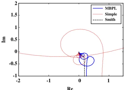
ε(s), to the controller from the equations (4), (5) and (6) for the three cases of simple control loop and the Smith predictor and the MBPL-predictor are shown in comparison in Fig. 7. In this figure the process model is selected to be Gp(s)=3exp(-s)/(s+1), and the MBPL-predictor is selected to be Gmb(s)=4/(s+1). This MBPL-predictor is selected to be gain dominant at all frequencies. Later, it will be discussed that any crossings of the gain of the predictor and the gain of the simple-open-loop-transfer-function will result in an inferior performance of the phase limiter predictor, due to the fact that after crossing of the gains the domination of the gain of the predictor will not prevail any more. It is seen in Fig. 7 that the simple-control-loop behaves in an unstable manner, while both of the predictors bring about stable condition, but with different dynamical behaviors.
ROBUSTNESS COMPARISON
In this part of the paper, robustness of the method is
Fig. 7: Comparison of the Nyquist plots of the error signals to the controller for a simple control loop with time-delay, Smith predictor used with a perfect model and a MBPL-predictor.
considered concerning the model mismatch. Error in model can be shown as [20]:
) s ( G ) s ( G ) s (
G = n +δ (8)
In equation (8), G(s) is the process transfer function and δG(s) is the difference of real transfer function and process nominal transfer function, Gn(s). Thus, δG(s) is the uncertainty in G(s). By substituting G(s) in the equation of closed loop response of three cases; simple feedback loop, Smith's method, as well as the proposed method, the following equations could be reached respectively.
) j ( G
) j ( G ) j ( G 1 ) j ( G
c n c
C ω
ω ω + = ω
δ (9)
) j ( G
) j ( G ) j ( G 1 ) j ( G
c 0 c
S ω
ω ω + = ω
δ (10)
) j ( G
) j ( G ) j ( G ) j ( G 1 ) j ( G
c
0 c mb
A ω
ω ω + ω +
= ω
δ (11)
Where, |δG(s)| is the norm bound uncertainty region [20] and is an scale to study the robustness of the method against the model's error by comparing equations(9), (10) and (11). It can be concluded that in equal conditions, the norm bound uncertainty region in the proposed method is larger than the Smith's method and the conventional simple feedback loops. Moreover the norm bound uncertainty region could be variable which indicates the high flexibility of this method.
2
1.5
1
0.5
0
-0.5
-1
Im
-2 -1 0 1
Re
Iran. J. Chem. Chem. Eng. A New Method for Time-Delay … Vol. 27, No. 4, 2008
Fig. 8: A crossing of gains of the predictor, Gmb(s)=4/(s+1), and the simple-open-loop-transfer-function, 3e-8s/s, appear at lower frequencies when using PI controller.
PI CONTROLLER
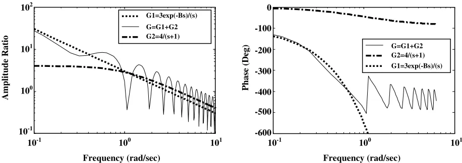
When using PI controller, there will appear special conditions in obtaining dominant gain for the predictor. The problem is that the simple-open-loop-transfer-function, which exists also in the irrational model of the MBPL-predictor loop, will exhibit a slope of -1 at low frequencies in AR as is shown in Fig. 8. Since the asymptote of the gain of the predictor has a slope equal to zero at low frequencies, there will always appear a crossing of the gains in spite of how much the gain of the predictor is increased. However, with increasing the gain of the predictor, the point of crossing will shift to the side of lower frequencies. The consequent of this crossing is that the average ultimate amount of the phase of the irrational model, at high frequencies, may overpass from what it would be when there is no crossing in the gains, as is evident by comparing the phases in Figs. 8 and 2-a,. Thus, the phase of the model will behave something between those of Figs. 2-a and 2-b. That is, while it does not behave exactly as a ULDRP, in the same time, it overpasses the limitation which will appear in the phase without existence of time-delay parameter. We call this behavior L-ULDRP, meaning that the model behaves like a ULDRP at lower frequencies, but changes to behavior of LDRP at higher frequencies. Thus, the conception of limited phase characteristics appears after some extra phase shift had occurred at lower frequencies. According to [14,15] this behavior corresponds to the condition where there are some limited numbers of right half plane zeros in the Ir-TF model. Anyway, it is important to choose and/or optimize the amount of the gain of Gmb(s)
such that the amount of the above mentioned phase overpass is minimized.
MBPL-PREDICTOR PROPERTIES
There are some specific properties of the proposed predictor which are important to be declared briefly here. These properties are discussed bellow.
Robustness to model error
Perhaps, it can be claimed that the most important property of the proposed predictor is its high robustness to model uncertainties. This is due to the fact that the robustness of the control loop and its stability under any situation is guaranteed only by making the gain of the predictor dominant comparing to the gain of simple-open-loop-transfer-function at all frequencies. A simple example will be used here for describing this property in comparison to the Smith predictor, when a considerable error appears in the time-delay parameter of the model.
In Fig. 9 an example is depicted for the closed loop response of a process with the exact model Gp(s)=4.5e-15s/(s+1) comparing to the approximate model,
) 1 s /( e 3 ) s (
Gˆp = −1s + for the process and the PI controller
Gc(s)=1+1/s In this figure, it is shown that a +55 % error in the gain and the time-delay can be stabilized in closed loop control with Kmb=6, but the severe overshoot and oscillatory behavior of the response improves greatly by using Kmb=8, while the performance of the Smith predictor is almost unacceptable. For the systems with high values of time-delay the effect of increased time-
102
101
100
10-1
A
m
p
li
tu
d
e
R
at
io
10-1 100 101 Frequency (rad/sec)
G1=3exp(-Bs)/(s)
G=G1+G2 G2=4/(s+1)
0
-100
-200
-300
-400
-500
-600
P
h
as
e
(D
eg)
10-1 100 101 Frequency (rad/sec)
G=G1+G2 G2=4/(s+1)
delay parameter can be compensated by increase in the value of Kmb for prevention of excessive overshoot and oscillation in the response.
The Method of Majhi & Atherton [12] is used for tuning of the Smith predictor in Fig. 9, with the amount of the parameters of controller being Kc=0.33, τi =1.
Capability to control distributed parameter process systems
A variety of distributed parameter process systems can be described by Ir-TFs, with the model structure as in equation (1). In such models, Smith predictor can not be used since the time-delay parameter can not be factored out explicitly. Contrary to the Smith predictor, MBPL-predictor can be applied for delay compensation of Ir-TF systems. An example is shown in Fig. 10 for closed loop response of the process model Gp(s)=[e-3s/(s+1)]+ [1/(s+1)], Gmb(s)=5/(s+1) and the PI controller, Gc(s)=1+1/s, with 0 % and +33 % and -100 % errors in the time-delay parameter. In this figure a load input equal to -0.1 is applied at time 70 sec. after the initial step input for set point.
Capability to control integrator systems with time-delay for load input
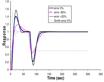
Another advantage of the MBPL-predictor is that it can be used for controlling load rejection of integrator processes with time-delay without any offset, while the conventional Smith predictor when used for such systems will result in some amount of offset. An example is shown in Fig. 11 for the model Gp(s)=e-5s/s and the MBPL-predictor Gmb(s)=32/(s+1) and the PI controller Gc(s)=4+0.2/s with 0.0 %, -80 % and +20 % error in time-delay parameter and step response to set point at time zero and load input equal to -0.1 at time 70 sec.
Capability to remove the effects of high order dynamics of the model
Similar to the time-delay parameter, high order dynamics of the model can become limited in phase and controlled robustly by the MBPL-predictor. This is shown in Fig. 12 for the process Gp(s)=e-4s/[(s+1)10], the predictor Gmb(s)=6/(s+1) and the PI controller Gc(s)= 2+0.4/s used controlling set point unit step input at time zero and load input equal to-0.1 at time 70 sec with zero percent error as well as ±25 % errors in time-delay and also ±25 % errors in gain.
Fig. 9: Closed loop response of the Smith predictor in comparison to the response of MBPL-predictor for different values of the predictor gain.
Fig. 10: Controlling the Ir-TF systems by MBPL-predictor.
Fig. 11: Response of the MBPL-predictor to step input in set point and load input for an integrator system with time-delay.
Time (sec)
0 10 20 30 40 50 60 2.5
2
1.5
1
0.5
0
-0.5
R
es
p
on
se
Gmb=6/(s+1)
Gmb(s)=8/(s+b)
Smith
R
es
p
on
se
-20 0 20 40 60 80 100 120
Time (sec) 1.2
1
0.8
0.6
0.4
0.2
0
-0.2
error 0 %
error -100 % error +33 %
0 0.2 0.4 0.6 0.8 1 1.2 1.4 1.6 1.8
0 50 100 150 200 250 300 350
Time (sec)
R
e
s
p
o
n
s
e
Iran. J. Chem. Chem. Eng. A New Method for Time-Delay … Vol. 27, No. 4, 2008
Fig. 12: Controlling high order models by MBPL-predictor.
Fig. 13: Gain domination of the selected MBPL-predictor, Gmb(s)=2/(s+1) compared to the model.
Variable time-delay processes
Since robustness properties of the proposed method, is much simple and clear, an important side-conclusion is worth noting here. That is, in cases when the time-delay is a varying parameter in the loop it would be much easy to design the predictor such that the loop works stable, without deficiency in its performance in a wide range of time-delay parameter variations. An example is useful here for investigating this problem.
For example we consider a process with following model:
) 1 s 5 . 0 )( 1 s )( 1 s 2 )( 1 s 3 (
e )
s ( G
s p
d
+ +
+ + =
τ
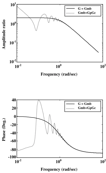
Where, the time-delay is supposed to vary in the range τd=20 to 26. At first for τd=26, Gmb(s)=2/(s+1) is selected. Fig. 13 shows that with this selection of
Fig. 14: Bode plots for the selected MBPL-predictor, Gmb(s)=2/(s+1) and the open loop.
Gmb(s)= 2/(s+1) the MBPL-predictor gain dominates the model gain at all frequencies. Now, based on ITSE integral criteria the controller is obtained as Gc(s)= 1.35+0.0768/s. In this case,asis shown in Fig. 14 Gmb(jω) is almost dominant at most of the frequencies so that phase curve is limited to less than -180 degree at high frequencies. In this way, one becomes satisfied that all of the zeros of characteristic equation will lie in the left half plane.
In Fig. 15 the proposed method response is shown for a single value of time-delay, τd=26. Also Kaya method [21] performance, which is an improved robust Smith predictor, is shown for comparison in this figure.
The tuning of controller for the method of Kaya is Gc(s)=0.315+0.0858/s. In principle the method of Kaya is a robust method with better performances compared to the other robust tuning methods for Smith predictor.
-50 0 50 100 150 200 250
Time (sec) 1.4
1.2
1
0.8
0.6
0.4
0.2
0
-0.2
R
es
p
on
se
Error 0 %
Time delay error +25 %
Time delay error -25 %
Gain error +25 %
Gain error -25 %
Gp-exp(-4s) / (s+1)10
10-1 100 101 102 Frequency (rad/sec)
105
100
10-5
10-10
A
m
p
li
tu
d
e
rat
io
G = Gmb G = Gp
10-2 100 102
Frequency (rad/sec) 101
100
10-1
10-2
A
m
p
li
tu
d
e
rat
io
G = Gmb Gmb+GpGc
10-2 100 102
Frequency (rad/sec) 40
20
0
-20
-40
-60
-80
-100
P
h
as
e
(D
eg.
)
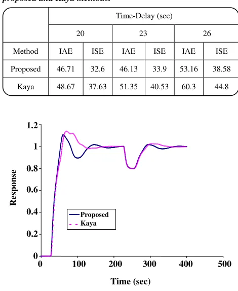
Table 1: IAE and ISE for the variable time-delays to the proposed and Kaya methods.
Time-Delay (sec)
20 23 26
Method IAE ISE IAE ISE IAE ISE
Proposed 46.71 32.6 46.13 33.9 53.16 38.58
Kaya 48.67 37.63 51.35 40.53 60.3 44.8
Fig. 15: Closed loop response of the Kaya method in comparison to the response of MBPL-predictor, ττττd=26.
For the variable time-delays, IAE and ISE integral errors are shown in table 1 for both methods using various amounts of time-delay in the range, τd=20 to 26. As is seen, while the calculated integral of error increases with increase of time-delay for both methods, the proposed method represents less error at all cases.
In the tuning method of Kaya, the high order models are estimated, using a relay test, by a first or second order transfer function. However, in the proposed method, the high order model is applied directly in controller tuning.
CONCLUSIONS
A new predictor is proposed which is based on the idea of dominating the gain of a first-order-without-time-delay predictor comparing to the overall gain of the remaining elements in the control loop. The idea of dominating the gain of the predictor, which has the capability to limit the effects of time-delay parameter and the non-minimum phase characteristics in the closed loop control system is concluded from the fact that in an irrational transfer function model (Ir-TF), which is known
to exhibit transcendental characteristics, or dual behavior in phase, it is possible to change the behavior of the model into the desired shape only by adjusting the gains of the elements of the model, such that the time-delay free element of the model becomes dominant in gain at all frequencies. Application of the idea, named model-bypass-phase-limiter-predictor (MBPL-predictor), to a simple feedback control loop, including time-delay, reveals some important properties of the predictor. The most important of the properties are:
a) - Achievement of robustness in control loop simply by adjusting the gain of the predictor. This feature in-corporates also the capability of the method for improved compensation of the variations of the time-delay parameter. b) - Capability to control distributed parameter process systems. c) - Capability to control integrator systems with time-delay for load input. d) - Capability to remove the effects of high order dynamics of the model.
APPENDIX
According to theFig.A-1 thethreevectors "C=G(jω)", "A= G1(jω)" and "B= G2(jω)" are considered for the model in (1) and its elements, in a specific frequency in the complexplanewith the respective angles "∠G(jω)=γ", "∠G1(jω)=α" and "∠G2(jω)=β". In this figure, it is supposed that vector "G1(jω)" is the dominant gain element of the model. For the purpose of proving that the vector "G(jω)" resonates around "G1(jω)" with increase of ω, and follows its behavior in frequency response, it would be sufficient to show that "|γ-α|≤|δ/2|=|(β-α)/2|" in the frequency band in which the vector "G1(jω)" is dominant in its gain; i. e., |G1(jω)|>|G2(jω)|. The equality condition in the above prevails when non of the vectors are dominant in its gain; i. e., |G1(jω)|=|G2(jω)|.
If the condition (γ-α)<(β-α)/2 prevails, then:
2 tg ) ( tg ) ( tg 1
) ( tg ) ( tg 2
tg ) (
tg < β−α
α γ +
α − γ α
− β < α −
γ (A-1)
Since that;
β +
α
β +
α =
γ
cos | B | cos | A |
sin | B | sin | A | ) (
tg then after
substitution in (A-1),
2 tg
cos sin cos | B | cos | A |
sin | B | sin | A | 1
cos sin cos | B | cos | A |
sin | B | sin | A |
α − β <
α α × β +
α
β +
α +
α α − β +
α
β +
α
(A-2)
0 100 200 300 400 500
Time (sec) 1.2
1
0.8
0.6
0.4
0.2
0
R
es
p
on
se
Iran. J. Chem. Chem. Eng. A New Method for Time-Delay … Vol. 27, No. 4, 2008
Fig. A - 1: Vector representation of the irrational model in (1) and the corresponding elements.
After some rearrangements of (A-2),
) sin sin cos (cos | B | ) sin (cos | A |
) cos sin cos (sin | B |
2 2
β α + β α +
α + α
β α − α β
(A-3)
2 tgβ−α
<
α − β α
− β < α − β +
α − β
2 cos 2
sin ) cos( | B | | A |
) sin( } B |
α − β
α − β
< α − β +
α − β α − β
2 cos
2 sin
) cos( | B | | A |
2 cos 2 sin | B | 2
(
)
1 cos
| B |
| A |
2 cos
2 2
< α − β +
α − β
The following simple relation will be obtained.
1 ) cos( | B |
| A |
) cos( 1
< α − β +
α − β +
(A-4)
The above inequality is valid since |A|>|B| is the initial assumption in this prove. In Fig. A-2 variations of
z=[1+cos(β-α)]
/
[|A|/|B|+cos(β-α)] with Y=(β-α) is drawn for various amounts of X=|A|/|B|.In Fig. A-2, ‘Z’ is indicator of angel's tangent between resultant vector and vector A, so ever X be larger than 1 (tangent of 45 degree angle) and be lesser this shows that X closes vector A but once X amount be less than 1 means 0.99 which shows that vector B is dominant, this
Fig. A - 2:Variations ofz=(1+cos(ββββ-αααα))/(|A|/|B|+cos(ββββ-αααα)) with Y=(ββββ-αααα) and X=|A| / |B|.
goes to extreme and means that the resultant vector becomes function B.
Then it is straightly realized that the resultant vector, i.e., the model vector, will be directed towards the higher gain element. Thus, in every frequency band, whatever the dominant gain element is, either the time-delay included element or the non-delay element, the resultant vector will be directed towards that one and will trace its behavior both in gain and phase characteristics.
Received : 3rd March 2008 ; Accepted : 16th June 2008
REFERENCES
[1] Smith, O. J. M., Closer Control of Loops with Dead-Time, Chemical Engineering Progress, 53, p. 217, (1959).
[2] Palmor,Z., “Stability Properties of Smith Dead Time Compensator Controllers”, Int. J. Control, 32 (6), p. 212, (1980).
[3] Hang, C. C., Lim, K. W. and Chong, B. W., A Dual - Rate Adaptive Digital Smith Predictor, Automatica, 25(1), p. 1 (1989).
[4] Watanabe, K. and Ito, M., A Process Model Control for Linear Systems with Time Delay, IEEE Trans. Automat. Contr., AC-26(6), p. 1261 (1981).
[5] Mataušek, M. R., Mici , A. D., A Modified Smith Predictor for Controlling a Process with an Integrator and Long Dead Time, IEEE Trans. Automat. Control,44(8), p. 1196 (1996).
[6] Mataušek, M. R., Mici , A. D., On the Modified Smith Predictor for Controlling a Process with an Im
O Re
β δ
γ α
A
C B
0 1 2 3 4 5 6 Y (rad)
3
2.5
2
1.5
1
0.5
0
N
X=0.99 X=3 X=1
Integrator and Long Dead Time, IEEE Trans. Automat. Contr., 41(8), p. 1603 (1999). [7] Hägglund, T., A Predictive PI Controller for Processes with Long Dead Times, IEEE Contr. Syst. Mag., 12(1), p. 57 (1992).
[8] Astrom, K., Hang, C. C. and Lim, B. C., A New Smith Predictor for Controlling A Process with an Integrator and Long Dead Time, IEEE Transactions on Automatic Control, 39(2), p. 343 (1994).
[9] Kaya, I., Atherton, D. P., A New PI - PD Smith Predictor for Control of Processes with Long Dead Time, in: 14th IFAC World Congress, Vol. C, p. 283, Beijing (1999).
[10] Kaya, I., Obtaining Controller Parameters for a New PI-PD Smith Predictor Using Auto Tuning, Journal of Process Control, 13(5), p. 465 (2003).
[11] Majhi, S., Atherton, D. P., Modified Smith Predictor and Controller for Processes with Time Delay, IEE Proc. Control Theory Appl., 146(5), p. 359 (1999).
[12] Majhi, S.¸ Atherton, D. P., Obtaining Controller Parameters for a New Smith Predictor Using Auto Tuning, Automatica,36(11), p. 1651 (2000).
[13] Xiang Lu,Yong Sheng Yang, Qing Guo Wang, Wei Xing Zheng, A Double Two Degree of Freedom Control Scheme for Improved Controlof Unstable Delay Processes, Journal of Process Control, 15(5), p. 605 (2005).
[14] Ramanathan, S., Curl R. L. and Kravaris, C., Dynamics and Control of Quasirational Systems, AIChE J., 35(6), p. 1017 (1989).
[15] Gundepudi, P. K., Friedly, J., Velocity Control of Hyperbolic Partial Differential Equation Systems with Single Characteristic Variable, Chem. Eng. Sci., 53(24) p. 4055 (1998).
[16] Shirvani, M., Inagaki, M. and Shimizu, T., A SimplifiedModel Of Distributed Parameter Systems, Int. J. Eng., 6(2), p. 65 (1993).
[17] Shirvani, M., Inagaki, M. and Shimizu, T., Simplification Study on Dynamic Models of Distributed Parameter Sytems, AIChE J., 41(12), p. 2658 (1995).
[18] Shirvani, M., Doustary, M.A., Shahbaz, M., Eksiri, Z., Heuristic Process Model Simplification in Frequency Response Domain, I.J.E. Transactions B: Applications, 17(1), p. 19 (2004).
[19] Toudou, I., Flow Forced Dynamic Behaviour of Heat Exchangers, Trans. JSME, (in Japanies) 33, p. 215 (1967).
[20] Morari, M. and Zafiriou, E., “Robust Process Control”, Englewood Cliffs, NJ: Prentice-Hall, (1989).