http://www.sciencepublishinggroup.com/j/ajmp doi: 10.11648/j.ajmp.20170604.13
ISSN: 2326-8867 (Print); ISSN: 2326-8891 (Online)
Green’s Functions Method in Problems of Sound Diffraction
Alexander Kleshchev
Department of Physics, Saint-Petersburg State Navy Technical University, Saint-Petersburg, Russia
Email address:
To cite this article:
Alexander Kleshchev. Green’s Functions Method in Problems of Sound Diffraction. American Journal of Modern Physics. Vol. 6, No. 4, 2017, pp. 56-65. doi: 10.11648/j.ajmp.20170604.13
Received: May 19, 2017; Accepted: June 2, 2017; Published: July 7, 2017
Abstract:
Initially, the Green’s functions method was used to solve the problem of the sound scattering on ideal scatterers with mixed boundary conditions. It was later applied to the sound diffraction studies on ideal and elastic bodies of the non-analytical form.Keywords:
Diffraction, Green’s Functions, Non-analytical Form, Boundary Conditions1. Introduction
The review set out in detail the use of Green’s functions method for diffraction problems on simple bodies (sphere, spheroid) with mixed boundary conditions. Analitical solutions are complemented by results of calculations of the scattered sound field similar bodies in zones of the Fresnel and Fraunhofer. In the future the method of Green’s functions has been extended to ideal and elastic scatterers of the non-analytical form.
2. The Sound Scattering of Bodies of the
Simple Form (Sphere, Spheroid) with
Mixed Boundary Conditions
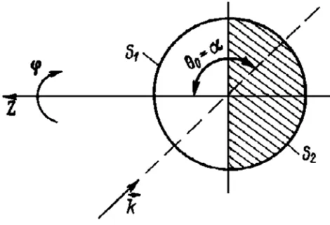
Ideal scatterers, that have on different parts of the surface are not the same boundary con-ditions (Dirichlet or Neumann), referred to bodies with mixed boundary conditions. Sound diff-raction problems on such scatterers are solved one two methods. The first proposed A. Sommerfeld [1], called the variational method (or the method of least squares) [1 – 3]. The second met- hod - the method of Green’s functions [4 – 7], is based on the use of the corresponding Green’s function with mixed boundary conditionsfor the each part of the surface of the scatterer. Lets look at an use and characteristics of both methods at an example of a sphere of a radius R with mixed boundary conditions (one half of a sphere is ideal soft, an other is ideal hard), that is on the area surface S1
(
θ = ÷0 90)
is perfomed the Dirichlet condition and in the area(
)
2 =90 180÷
S θ - the Neumann condition (Figure 1). In accordance with given boundary conditions by using a varia-tional method is made a functional GN of the form [1]:
1 2
2 2
2
.
∂Φ ∂Φ
= Φ + Φ + +
∂ ∂
∫
∫
N i s
i s
S S
G k dS dS
n n (1)
where k – the wave number of the incident plane wave.
Figure 1. The sphere with mixed boundary conditions.
(
)
(
) (
) (
)
(
) (
0 0) ( )
; ; 2 1 ! !
cos cos cos ;
∞ −
= =
Φ = + − + ×
×
∑∑
m ni m
m n
m m
n n n
r i n n m n m
P P j kr m
θ φ ε
α θ φ
(2)
(
)
(
)
( )1( )
0 0; ; cos cos ,
= =
Φ =
∑∑
N v v vs q q q
v q
rθ φ A P θ h kr vφ (3)
where Aqv - unknown coefficients of expansions,
1, 0;
2, 0 .
= = ≠ m m m ε
In expanded form a functional GN
is [4, 5]:
(
)
(
) (
) (
)
(
) ( )
(
)
( )( )
(
)
(
) (
)
(
) (
) ( )
1
1 1 1
1 1 1 1
1 1 1 1 1 1 2 2 2 2 0 0 0 0 1 0 0
1 1 1 1 1
0 0
1
2 1 cos ! ! cos
cos cos cos
2 1 ! ! cos cos
cos c ∞ − = = = = ∞ = = = × × + − + × × + × × + − + × × +
∑∑
∫ ∫
∑∑
∑ ∑
N mn m m
m n n n
m n
N v
v v
q q q
v q m
n m m
m n n n
m n
v v q q
G k R
i n P n m n m P j kR
m A P h kr v
i n n m n m P P j kR
m A P
π π ε α θ φ θ φ ε α θ φ
(
)
( )( )
(
)
(
) (
) (
)
(
) ( )
(
)
( )( )
(
)
(
) (
)
(
) (
)
1 1 1 11 1 1
1 1 1
2 1 0 0 2 2 0 0 0 2 1 0 0
1 1 1 1 1
os cos sin
2 1 cos ! ! cos
cos cos cos
2 1 ! ! cos cos
= = ∞ − = = ′ = = + ′ + + − + × × + × ′ × + − +
∑ ∑
∑ ∑
∫ ∫
∑∑
v N q v q mn m m
m n n n
m n
N v
v v
q q q
v q
n m m
m n n n
h kR v d d
R i n P n m n m P j kR k
m A P h kR k v
i n n m n m P P j
π π π θ φ θ θ φ ε α θ φ θ φ ε α θ
( )
(
)
( )( )
1 1 1 1 1 1 11 1 1
1 1
0 0
2
1 1
0 0
cos cos cos sin ,
∞ = = ′ = = × × +
∑ ∑
∑ ∑
m m n v N v vq q q
v q
kR k
mφ A P θ h kR k vφ θ θ φd d
(4)
Where a feature over unknown coefficients means a sign of a complex conjugation.
The minimization condition of a functional N
G ensures best execution of boundary con-ditions on a surface of a scatterer:
0.
∂ N ∂ =i
i
G A (5) The substituting (4) in (5), obtain equations for a determining of unknown coeffici-ents Aqv:
1 1
0 0 0 0
,
= = = =
= −
∑∑
N M v vv∑∑
N M vvq qq nq
v q n q
A C d
where M – the integer index, whose value depends on the size of the wave kR;
( )
( )
(
) (
)
( )( )
( )( )
(
) (
)
1 1 1 1 2 1 0 1 2 2cos cos sin
cos cos sin ;
′ ′
= ∆ +
+ ∆
∫
∫
vv v v
qq q q q
v v
q q q q
C h kR v P P d
h kR h kR v P P d
π π π θ θ θ θ θ θ θ θ
(
) (
) (
)
(
)
( )
( )( )
(
) (
)
( )
( )( )
(
) (
)
1 1 1 1 1 2 2 0 2 22 2 1 ! ! cos
cos cos sin
cos cos sin ;
′ = + − + × × + ′ +
∫
∫
vv n v
nq n
v v
n q n q
v v
n q n q
d i n n v n v P
j kR h kR P P d
j kR h kR P P d
π π π α θ θ θ θ θ θ θ θ
2, 0 ;
1, 0 ,
= ∆ = ≠ v v v
On the other hand, in accordance Green’s functions method [6] a potential of a scattered wave Φsby a sphere with mixed
boundary conditions represented by a one-term the in-tegral Huygens as a sum:
( )
(
)
(
)
( )
(
)
( )
(
)
1 2 1 1 2 2 ; ;1 4 ,
, , Φ = Φ = ′ = − Φ ∂ ∂ + ′ + ∂Φ ∂
∫
∫
s s i S i S P rQ G P Q r dS
Q r G P Q dS
θ ϕ
π
(6)
φ; Q – the surface point with angular coordinates φ θ′′ ′′, and a radial coordinate r′ =R; G1 – the Green’s functionvanishes
on the surface of a scatterer аnd G2 – the Green’s function
having a zero derivative along the normal to this surface [8, 9]:
(
)
(
) (
)
(
) (
) (
)
(
)
( )
( )( )
( )( )( ) ( )
( )( )
10 0
1 1 1
; ; ; ; ; 2 1 cos
cos ! ! cos
; ∞ = = ′ ′ ′ = + ′ × ′ × − + − × ′ ′ × −
∑∑
m mm n
m n
m n
n n n n n
G r r ik n P
P n m n m m
j kr h kr h kr kr j kR h kR
θ φ θ φ ε θ
θ φ φ (7)
(
)
(
) (
)
(
) (
) (
)
(
)
( )
( )( )
( )( )
( )( ) ( )
( )( )
20 0
1 1 1 1
; ; ; ; ; 2 1 cos
cos ! ! cos
. ∞ = = ′ ′ ′ ′ = + ′′ × ′ × − + − × ′ ′ ′ × −
∑∑
m mm n
m n
m n
n n n n n n
G r r ik n P
P n m n m m
j kr h kr h kr h kr j kR h kR
θ φ θ φ ε θ
θ φ φ (8)
The formula (6) for a potential Φs
(
r; ;θ φ)
of a scattered wave, is approximate as a formula (4) of a variational method. But there are special cases in which a Green’s functions method gives accurate results. We will consider these special cases on the example of the homoge-neous (soft) sphere, visualizing her broken into two halves by a plane XOZ (Figure 1). The wave vectork
of the incident plane wave put in a plane XOZ (θ
0=
90
) and put it in a same the observationpoint P (on a contour of a border of hemispheres S1 and S2).
We will find
Φ
s( )
P
in this point, using on a left hemisphere S1 the Green’s function G1 and on a right hemisphere S2 - theGreen’s function G2.
For a homogeneous soft sphere a formula (6) converted to a form:
( ) (
)
( )
(
)
( )
(
)
1 2
1 1 2 2
1 4 , , ,
′ ′
Φ = − Φ ∂ ∂ + ∂Φ ∂
∫
∫
s i s
S S
P π Q G P Q r dS Q r G P Q dS (9)
where:
( )
(
)
(
) (
)
(
) (
)
( )( )
( )
( )( )
1 0 0 12 1 ! ! cos cos cos
. ∞ − = = ′ ′ ′ Φ = − + − + × ′ ×
∑ ∑
m n m ms m n n n
m n
n n
Q i n n m n m P P m h kr
j kR h kR
ε α θ φ
Using Φs
( )
Q and G1, G2 from (7) and (8), we find that apotential of a scattered wave on a surface of a sphere in a point of a contour of a border of two hemispheres is equal:
( )
( ) ( ) ( ) ( )
1 2 1 2( )
,Φs P = − Φi P − Φi P = −Φi P
That is a boundary condition is fulfilled and a solution is accurate.
If still a sphere θ0 and θ = 90о, a sphere consists of soft and
hard hemispheres (Figure 1), the, contribution of the ideal soft hemisphere in a potential Φs in the point of a contour of a
border is equal Φi
( )
P 2, but the contribution of the ideal hard hemisphere ∂Φ ∂s r in on a contour of a border is equal( )
(
)
1 1
2− ∂Φ P ∂r . The potential Φs in the plane XOZ will be
equal to half a sum of potentials generated by soft and hard spheres in a same plane.
Arbitrary orientation of a wave vector k of the incident wave with respect to an our sphere with mixed boundary conditions a potential of a scattered wave Φs
(
r; ;θ φ)
will by equal approximate by substituting (2) in (7) and (8) in (6) [7]:(
)
( )
(
) (
) (
)
(
)
(
)
( )( )
{
( )
( )( )
( )
( )( )
}
( )
( )
(
)
(
) (
) (
) (
) (
)
(
) (
)
( )( )
( ) ( )
1 1 1 0 01 1 1
0 0 0
1
1 1 1
; ;
1 2 2 1 ! ! cos cos cos
1 2 1 2 1
2 1 ! ! ! ! cos cos cos
0 0 ∞ − = = ∞ ′ − = = = ′ Φ = = + − + × ′ × + + − + × × + − + − + × ×
∑∑
∑∑ ∑
s mn m m
m n n
m n
m m
m n
n n n n n m
m n n
m m
n n n
m m
n n
r
i n n m n m P m P
h kr j kR h kR j kR h kR i n
n n m n m n m n m m P P h kr
P P θ φ ε θ φ α ε φ θ α
( ) ( )
(
) (
)
{
}
( )
( )( )
( )
( )( )
{
1}
1 1
1 1
1 1
0 0 1 1
, ′ ′ − + − + × ′ × − + m m n n
n n n n
P P n n n n
j kR h kR j kR h kR
(10)
Figure 2. The distribution of the module of the potential of the scattered wave on the surface of the sphere with mixed boundary conditions^ 1 – the variational method; 2 – the met-hod of Green’s functions.
In contrast to a variational method in a method of Green’s functions does not need to look for unknown coefficients of expansions and a computation of a potential Φs is a very
simple problem, since all quantities in (10) are known. On fiure. 2 shows distributions of Φs on a surface of a sphere
(half-soft S1, half-hard S2) by kR = 5 and
α
= 90о. The idealsoft half of a sphere corresponds change of an angle θ ina range of 0 to 90°. The single value of a potential of a mo-dule shown dash-dotted arc, it complies with a strict implementation of a boundary condition on a surface of a sphere satisfied approximately although a difference is small between methods themselves.
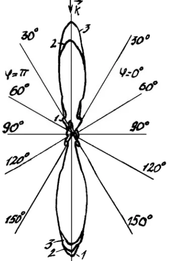
Figures 3 and 4 show amplitude angle characteristics of a soft (figure 3, a curve 1) and hard (fiure. 4, a curve 3) spheroids and the angle characteristic of a spheroid with mixed boundary conditions (Figures 3 and 4, a curve 2).
Figure 3. Angular characteristics.
Figure 4. Angular characteristics.
If, for example, to introduce a prolate spheroid consisting of two identical halves, con-tacting in a plane η= ⇔ =0 θ 90 and in a same plane (η0 =0) to place a source, a total potential
Φs of a scattered field for a observation point, of which is in a
same plane η=0. Will be determined to expressions (11) (φ=0) and (12) (φ π= )
(
)
(
)
( )
( )( )
( )
(
)
( )
(
)
( )
(
)
( )
(
)
3
, 1 , ,
0
1 1
, 0 , 0
3 3
, 0 , 0
; ; 0 , , ,
, ,
,
, ,
∞ ∞
−
≥ =
′
′
Φ = ∈ ×
× +
∑ ∑
ns m m n m n m n
n m m
m n m n
m n m n
i S c S c R c
R c R c
R c R c
ξ η η η ξ
ξ ξ
ξ ξ
(11)
(
)
(
)
( )
( )( )
( )
(
)
( )(
)
( )
(
)
( )
(
)
3 2
, 1 , ,
0
1 1
, 0 , 0
3 3
, 0 , 0
; ; , , ,
, ,
.
, ,
∞ ∞
−
≥ =
′
′
Φ = ∈ ×
× +
∑ ∑
m ns m m n m n m n
n m m
m n m n
m n m n
i S c S c R c
R c R c R c R c
ξ η π η η ξ
ξ ξ
ξ ξ
(12)
Figure 5. Relative backscattering cross sections of oblate spheroids by
irradiating them along the axis of the rotation.
0,1005) they are irradiated along an axis of a rotation Z
(θ0 =0 ). A curve 4 relates to a hard half spheroid, a half soft,a curve 2 – to an ideal soft spheroid, a curve 1 – to an ideal hard spheroid, a curve 3 – to a spheroid, which, 1/3 a surface corresponds to a Neumann condition and 2/3 – a Dirichlet condition/
Figure 6 shows of a module of the angular characteristic
( )
s
ψ η of the oblate spheroid with a radial coordinate
ξ
0=0,1005 half-hard, half-soft (a curve 1), which falls a wave along the axis Z (θ0 =0 ⇔η0 =1, 0) by С=10; here given modules ψ ηs
( )
for soft (a curve 2) and hard (a curve 3)spheroids. A comparison of three curves chows that the amplitude of a pressure in a reflected back wave for a combined body by approximately one order smaller than for homogeneous ideal spheroids.
Figure 6. Modules angular scattering characteristics combined and
homogeneous oblate spheroids.
Figure 7. The non-analytical smooth scatterer in the form of the cylinder with
the semi-spheres.
3. The Method of Green’s Functions for
Ideal Scatterers of Non–analytical
Forms
We consider non-analytical body, the surface of which does not apply to coordinate symones with divided variables in the scalar Helmholtz equation. We examine this non-analytical scatterer in the form of a finite circular cylinder bounded on the sides of the hemispheres (figure 7).
Sound pressure, scattered by this body, can be found one of the numerical methods for the solution of diffraction problems [6, 7, 10 – 20]. The method of Green’s f functions [6, 7], based on the use of mathematical formulation of the principle of Helmholtz-Huygens (Kirchhoff integral), one of the most convenient methods. The algorithm of calculation requires knowledge of the amplitude-phase distribution of the sound pressure and the normal component of oscillatory velocity on some closed surface integration of S, that includes the lateral surface of the cylinder S2 and the surface of hemispheres S1 and S3 (Figure 7).
( ) 1
( ) [ ( ) ( , ) ( , )]
4
∂ ∂
= −
∂ ∂
∫
SS S S
p Q
p P p Q G P Q G P Q dS
n n
π , (13)
where ps (P) - the sound pressure scattered by the body, P -the
point of observation, which has a spherical coordinates: ; Q - the point of the surface S; ps(Q) - the sound pressure in
the point Q; G(P,Q) - Green's function of the free space, satisfying the inhomogeneous Helmholtz equation.
In the (13) Green's function is selected as a potential point source:
, (14) where k = – the wave number, - the length of a sound wave in the liquid environment, R - the distance between the points P and Q.
Using relative arbitrariness of the choice of Green's function, you can get the Kirchhoff formula options, consisting of a single member:
(1) 1
( ) ( ) ( , )
4
∂ =
∂
∫
S S S
p P p Q G P Q dS
n
π (15)
( 2) ( ) 1
( ) ( , )
4
∂ = −
∂
∫
SS S
p Q
p P G P Q dS
n
π (16) By using formulas (15), (16) is considerably simplified computational procedure: you want to define only one of the parameters (ps(Q) or dps(Q)/dn)on the surface S. However, in
The possibility of such a method and test calculations of the scattered field were considered in [21, 22]. For example, an experiment at the decision of a test problem [21] for the calculation of the far field of a point source (group of point sources) directly and through (24), (25) has shown that in the considered range of wave sizes of the results obtained by these two methods, goodenough coincide. When solving the problem of diffraction to determine the values of ps (Q) and dps(Q)/dn on
the surface S you can use the following expression:
1)for the homogeneous Dirichlet conditions (ideally soft body), the scattered pressure on the surface S has the form:
, (17) 2)for the homogeneous Neumann conditions (ideally rigid
body):
( ) ( )
,
∂ =∂
∂i ∂s
p Q p Q
n n (18)
where p, (Q) - the sound pressure of the incident wave in point
Q. When determining the values pt (Q) you can use the
expression for the scalar potential of the plane monochromatic wave single amplitude of the incident on the body from a source located at infinity.
This potential for a perfectly reflective sphere is natural functions in solving the Helmholtz equation in a spherical coordinate system has the following form [12]:
0 0
( )!
( , , ) (2 1) cos (cos ) ( );
( )!
∞ −
= =
−
= +
+
∑∑
n n mi n n n
n m
n m
p r i n m P j kr
n m
θ ϕ ε ϕ θ (19)
the expression (19) is simplified when considering the axis-symmetric problem (dependence on the coordinate
0
( , ) (2 1) (cos ) ( ),
∞ −
=
=
∑
m +i m n
m
p r
θ
i n Pθ
j kr (20)for scatterer in the form of a perfectly reflecting cylinder scalar potential incident plane harmonic waves unit amplitude of the wave vector, , aimed at the angle to the z axis of the cylinder, folding natural functions solutions to the Helmholtz equation in a circular cylindrical coordinate system:
(1) 0 0
0 0 (1)
0 0 0
( sin )
( , , ) exp( cos ) ( 1) ( ) cos ,
( sin )
∞
=
Ω
= − −
Ω
∑
m mi m m
m m
I kr
p r z ik z H kr m
H kr
θ
ϕ θ ε ϕ
θ (21)
in the case of the plane problem of the wave vector к perpendicular to the z axis of the cylinder and expression (30) is simplified [12]:
(1) 0 0
(1)
0 0 0
( sin )
( , ) ( 1) ( ) cos ,
( sin ) ∞
=
Ω
= − −
Ω
∑
m mi m m
m m
I kr
p r H kr m
H kr
θ
ϕ ε ϕ
θ : (22)
4. Results of Numerical Experiments
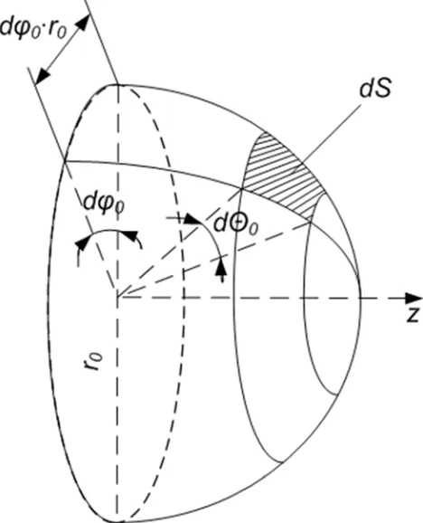
For calculation of integral (15) and (16) on the surface S the quadrature formulas is used. A step of integration over the surface S in the axial and circumferential directions in the system of nodal points must not exceed 0,5 (Figures 8, 9).Figure 8. The coordinate system, connected with cylinder.
Using the method of Green's functions were calculated the equivalent radius of the ideal non-analytical body for several values of wave size ka (where a is the radius of cylinder and hemispheres of the non-analytical scatterer) and different angles of irradiation (figures 10 – 12)
Figure 10. Angular diagrams R for the angle of the incident eq. 0 0=90 .
θ
Figure 11. Angular diagrams for the angle of the incident θ0=60 .0
Figure 12. Angular diagrams for the angle of the incident 0
0=30 .
θ
The analysis of equivalent radiuses presented on these pictures, permit to make the following conclusions:
1)the angular position of reflecting and diffraction lobes totally correspond to the physical representations; 2)the angular characteristics of submarine
non-analytical object are rather similar to the angular diagrams of spheroid bodies [4, 10].
At all figures clearly observed diffraction (shadow) petal, and it grows and shrinks with increasing frequency. On figures 10 – 12 the mirror petal is shows, which is similar to the shadow petal with increasing frequency, but in contrast,
5. The Green’s Functions Method for
Elastic Scatterers of Non–analytical
Forms
The solution of the problem of the sound scattering by an elastic shell of the non-analytical form is based an article [27]. The Green’s functions method is approximate because it does not take account the interaction between individual elements forming a compound body of non-analytical form. The interaction between scatterers shaped as spheroids and elliptic cylinders in [10] and this interaction was negligibly small. In addition, the sound scattering characteristics calculated for bodies with mixed boundary conditions by the Green’s function method namely the Sommerfeld method (the method of un-determined coefficients [10, 23]), and the agreement between the results was fairly good.
As non-analytical bodies considered two structures: 1)a finite-length circular cylindrical elastic shell limited an
the ends by the two halves of a prolate spheroidal shell (Figure 13);
2)the same end cylindrical shell bounded an the ends by the two halves of a spherical shell (Figure 14).
Figure 13. The cylindrical shell with the semi-spheroidal shells.
Figure 14. The elastic shell in the form of the terminal cylinder with the semi-spheres.
In article [27] given a decision acoustic scattering problems to the constituent parts of noana-lytical bodies.For cylindrical and spheroidal shells are used Debye and Debye-type potentials. In [27] the angular scattering characteristics of such com-pound bodies with different wave sizes are calculated.
We consider a compound elastic shell forme by a finite cylindrical shell whose ends are closed by two hemi spherical shells of the same diameter (figure 14). To apply the Green’s
function method, it is necessary to take the solution to the axi-symmetric problem of plane wave diffraction by an elastic spherical shell in terms of dynamic elasticity theory [28] and transform this solution to the three-dimensional version. The resulting solution little differs from that obtained above for the three-dimensional problem of diffraction by a spheroidal elastic shell [10, 23, 24, 29].
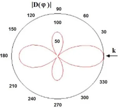
Figures 15 and 16 show the absolute values of the angular characteristics (in the XOY plane, =900) for non-analytical elastic scatterer in the form of a cylindrical shell connected with to spherical shells (figure 10) the following parameters: ka=0,523 (Figure 15) and ka=0,941 (Figure 16).
Figure 15. The modulus of an angular characteristic.
Figure 16. The modulus of an angular characteristic.
The method of Green’s functions in combination with analytical methods can be used for the solution of tasks of diffraction of plane sound wave on elastic isotropic scatter of non-analytical form, that consists of circular cylindrical shell of terminated length L and radius r0, bounded at the butts by
– by coordinate .
The shell material is isotropic, with the density and coefficients of Lame , module of Jung E, inside is the gas with density and coefficient of volumetric compression and sound rate .
The scatterer is placed in ideal compressed liquid with density and coefficient of volumetric compression The potential of sound wave is submitted to scalar equation of Helmholtz.
The amplitude-phase distribution of the sound pressure and of normal component of vibrating velocity in the points of this non-analytical surface is found from the strict solution of tridimensional boundary tasks of dynamic theory of elasticity on the endless elastic cylindrical surface and elastic spheroidal surfaces, respectively.
The schemes of solution of axially symmetric tasks of diffraction on elastic cylinder and spheroid are rather similar: in both cases the vector potential has the single nonzero component . The unknown coefficients of potentials’ expansion of falling and dispersed waves, of scalar potential of the surface, of potentials of Debye U and V, as well as of potential of gas, filling the surface, are found from the physical boundary conditions on the external and internal surfaces of the shell [30].
Although on the spheroid these coefficients are found not in the enclosed form, but using the method of truncation from the infinite system of equations.
What is more, while finding the solution of tridimensional task of diffraction on elastic speroidal scatterer the vector potential is presented by the potential of Debye U and V [10, 19, 30]:
2
( ) ( ),
Ψ =rotrot RU +ik rot RV (23) where – is the radius-vector of the view point of, – is the wave number of transverse wave in the material of the shell.
The sound pressure in the far-field can be found by one of the numerical methods, among those is the comfortable method based on the usage of mathematical formula of Helmholtz –Huygens ’ Principle (integral of Kirchhoff) [23]:
1 1 1
exp( )
( ; ; ) (1 / 4 ) {[ ( ) / ]
exp( )
( )( )[ ]}
= ∂ ∂
∂ −
∂
∫∫
s s
S
s
ikr
p r p Q n
r ikr
p Q ds
r r
θ ϕ π
(24)
where r – is the distance between the point Q on the surface of the shell and the point P with coordinates r1, θ1, φ1 in the far-field.
The Green’s functions in (14) is taken in the form of potential of the point-source. The quadrature formulas are used for finding of this integral, and here the integration step (sampling) of the surface of the scatterer should not exceed 0,5 λ0, where λ0 – is the length of the plane monochromatic
wave, falling from the liquid onto the surface of the scatterer.
6. Conclusions
The author of a Green’s functions method [6] analyzes him in this review on an example of sound diffraction problems on bodies with mixed boundary conditions and non-analytical forms. Initially. The Green’s function method was proposed for sound scattering problems on analytical bodies (sphere, spheroid) with mixed boundary conditions and it was shown in what cases this approximate method turns out to be accurate. Then this method was extended to solving problems of diffraction of sound on elastic bodies of non-analytical forms.This analysis is supplemented with calculations of characteristics of the sound scattering by ideal and elastic scatterers.
Acknowledgments
The work was supported as part of research under State Contract no P242 of April 21, 2010, within the Federal Target Program “Scientific and scientific - pedagogical personnel of innova-tive Russia for the years 2009 – 2013”.
References
[1] A. Sommerfeld. Differential equations in partial derivatives of the physics. Moscow: IL, 1950 [in Russian].
[2] M. I. Karnovskyi, V. G. Lozovik. Acoust. journal. 10, 313 (1964).
[3] M. I. Karnovskyi, V. G. Lozovik. Acoust. journal. 11, 176 (1965).
[4] A. A. Kleshchev. J. Mar. Gazette. 2, 94 (2013).
[5] E. B. Itkina, A. A. Kleshchev. Acoust. journal. 28, 414 (1982). [6] A. A. Kleshchev. Acoust. journal. 20. 632(1974).
[7] A. A. Kleshchev. Proc. LKI. Acoustics of ships and oceans. 19(1984).
[8] E. Skuchik. Principles ofacoustics. Moscow: Mir. V. 1, 1974 [in Russian].
[9] H. Hoenl, A. Maue and K. Westppfahl. Theorie der beugung. Berlin: Springer, 1961.
[10] A. A. Kleshchev, Hydroacoustic scatterers. St. Petersburg. Prima, 2012 [in Russian].
[11] A. A. Kleshchev. I. J. M. A., 2, 124 (2012).
[12] A. A. Kleshchev, Tr. LKI “The Сommon Ship’s Systems”. 95 (1989).
[13] A. E. Seybert, T. W. Wu and X. F. Wu X. F, J. Acoust. Soc. Am. 84, 1906 (1988).
[14] A. A. Kleshchev. Zeit. Fur Naturf. A. 6, 419 (2015).
[16] V. D. Kupradzc. Methods of potentials in the theory of elasticity. Moscow: Fizmat-giz, 1963 [in Russian].
[17] J.-H. Su, V. V. Varadan, V. K. Varadan, L. J. Flax. Acoust. Soc. Am. 68. 685(1980).
[18] A. Yu. Dushin, S. L. Il’mcnkov, A. A. Kleshchev, V. A. Postnov. Proc. of Symp. Tallinn. 89(1989).
[19] B. Peterson, S. Strom. J. Acoust. Soc. Am. 57. 2(1975).. [20] S. K. Numrich, V. V. Varadan, V. K. Varadan. J. Acoust. Soc.
Am. 70. 1407(1981).
[21] A. A. Kleshchev. J. of Techn. Acoust. 2. 65 (1993).
[22] S. L. Il’menkov. Proc. of the IV Far Eastern conference on acoustics. Vladivostok. 73 (1986).
[23] A. A. Kleshchev, I. I. Klukin. Principles of hydroacoustic.
Leningrad: Shipbuilding, 1987 [in Russian].
[24] A. A. Kleshchev. Diffraction and propagation of waves ineElastic mediums and Bo-dies. St.-Petersburg. Vlas, 2002 [in Russian].
[25] S. L. Il’menkov, A. A. Kleshchev. A. S. P. 2.50(2014). [26] S. L. Il’menkov, A. A. Kleshchev, A. S. Klimenkov, F. F.
Legusha, V. S. Mayorov, G. V. Chizhov, V. Yu. Chizhov. Proc. XXVII session RAO. 1(2014).
[27] S. L. Il’menkov, A. A. Kleshchev, A. S. Klimenkov. Phys. Acoust.. 60. 617(2014).
[28] A. A. Kleshchev, S. A. Klimenkov. A. S. P. 1. 68(2013). [29] A. A. Kleshchev. Diffraction, radiation and propagation of