Simulation Studies of Shock Formation due to Interactions of Two Plasmas in a Magnetic Field and Modified Two-Stream Instabilities

(1)

Department of Physics, Nagoya University, Nagoya 464-8602, Japan

(Received 26 November 2013/Accepted 28 February 2014)

Shock formation due to interactions between exploding and surrounding plasmas and evolution of modi-fied two-stream instabilities are studied using two-dimensional (2D) electromagnetic particle simulations. After the exploding ions penetrate the surrounding plasma, a strong magnetic-field pulse forms near the front of the exploding plasma. Because of modified two-stream instabilities, electromagnetic fluctuations grow to large am-plitudes in this pulse. AtΩit1, whereΩiis the ion cyclotron frequency, the pulse starts to reflect ions and to

split into two pulses, which then develop into forward and reverse shock waves. For various values of the initial exploding plasma velocity and of the angle between the velocity and external magnetic ﬁeld, 2D simulations are performed. The parametric dependence of the properties of the generated pulses and of magnetic ﬂuctuations is discussed.

c

2014 The Japan Society of Plasma Science and Nuclear Fusion Research

Keywords: collisionless shock, modiﬁed two-stream instability, whistler wave, particle simulation DOI: 10.1585/pfr.9.3401035

1. Introduction

Strong disturbances, such as solar flares and super-nova explosions, can generate shock waves via interactions between exploding and surrounding plasmas. When the plasmas are collisionless, shock formation processes are complex and are strongly influenced by the presence of an external magnetic field [1, 2]. In Ref. [3], the interactions between exploding and surrounding plasmas in an external magnetic field have been studied using theory and simu-lations for the case in which the initial velocity of the ex-ploding plasmav0is perpendicular to the external magnetic

ﬁeldB0. The shock formation processes were the

follow-ing. After the exploding ions penetrate into the surround-ing plasma, the explodsurround-ing ions induce an electric ﬁeld in the direction−v0×B0, which accelerates the surrounding

ions in this direction. Then, the directions of the ion veloc-ities significantly change because of the magnetic force, and a strong magnetic-field pulse forms near the front of the exploding ions. This pulse reflects the surrounding ions forward and exploding ions backward, which causes the splitting of the pulse into two pulses going forward and backward. These pulses subsequently develop into forward and reverse shock waves.

The above mentioned theoretical and simulation ap-proaches were one-dimensional (1D). Recently, using two-dimensional (2D) electromagnetic particle simulations, we conﬁrmed that essentially the same phenomena as in the

author’s e-mail: [email protected]

∗)_{This article is based on the presentation at the 23rd International Toki}

Conference (ITC23).

1D simulations occur in the 2D simulation for a case in whichv0is perpendicular toB0[4]. Furthermore, we have

investigated the evolution of modiﬁed two-stream instabil-ities, which were not included in 1D simulations. In this study, we also investigated the interactions between ex-ploding and surrounding plasmas using 2D simulations. After describing the evolution of the magnetic ﬁeld for a case ofv0being perpendicular toB0, we discuss the

simu-lation results for various values ofv0andθ, whereθis the

angle betweenB0andv0.

2. Simulation Model and Parameters

We use a 2D (two spatial coordinates and three velocity components) relativistic electromagnetic parti-cle code with full ion and electron dynamics. A uni-form external magnetic ﬁeld is in the (x,z) plane, B0 =

(B0cosθ,0,B0sinθ). The simulation plane is (x,z) with a

sizeLx×Lz=8192Δg×512Δg, whereΔgis the grid spacing.

The system is periodic in thezdirection and is bounded in thexdirection. The total number of simulation particles is N1.1×109_.

As initial condition, we used an exploding plasma with ﬂuid velocity v0 = (v0,0,0) in the region x < b

and a surrounding plasma at rest in the region x > b. This boundary is setb = 3300Δg. The initial density

ra-tio of exploding to surrounding plasmas isnE0/nS0 = 2.

The ion-to-electron mass ratio ismi/me =200. The light

speed isc/(ωpeΔg)=4.0, and the electron and ion thermal

velocities in the upstream region are vTe/(ωpeΔg) = 0.5

andvTi/(ωpeΔg) = 0.035, respectively, where ωpe is the

c

2014 The Japan Society of Plasma

(2)

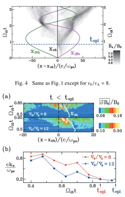
Fig. 1 Contour map of ¯Bz(x,t) in the (x,t) plane and trajectories of ions and electrons that were initially atx=b, forθ= 90◦andv0/vA=12.

electron plasma frequency averaged over the entire region. The magnetic ﬁeld strength is|Ωe|/ωpe = 0.5; hence the

Alfvén speed isvA/(ωpeΔg) = 0.14. We consider cases

forv0/vA<(mi/me)1/2, for which the modiﬁed two-stream

instabilities are more unstable than the ion Weibel instabil-ities [4].

3. Evolution of Magnetic Field

We brieﬂy describe the evolution of magnetic ﬁeld due to interactions between exploding and surrounding plas-mas using data forθ=90◦andv0/vA=12. Figure 1 shows

the contour map of ¯Bz(x,t) in the (x,t) plane, where ¯Bzis thez-averagedBzdeﬁned as

¯

Bz(x,t)= 1 Lz

dzBz(x,z,t). (1)

xiEb(pink line) is the averaged trajectory of ions that were

initially at the front of the exploding plasma, while xiSb

(green line) is for ions that were at the end of the surround-ing plasma. Explodsurround-ing and surroundsurround-ing electrons do not mix because they move withE×Bdrift [3]. Their bound-ary is denoted byxeb. The time in the left and right axes

is normalized toΩi0 andΩiE, respectively. Ωi0 is the

cy-clotron frequency of the surrounding ions in the upstream region, whileΩiE is that of the exploding ions with initial

speedv0, which is deﬁned as

ΩiE=Ωi0(1−v02/c2)1/2. (2)

In the early stageΩi0t <1, the exploding ions

pene-trate the surrounding ions and are decelerated because of thev×Bforce. This intensiﬁes ¯Bz in the region xeb <

x <xiEb, and a strong magnetic-ﬁeld pulse is formed. At

t=tspl, which is shown by the horizontal dashed line, this

pulse splits into two pulses, which then develop into shock waves, one propagating forward in the surrounding plasma away from xeb and the other backward in the exploding

plasma. This splitting is caused by ion reﬂection.

We now consider the 2D structure ofBz. In the region xiSb < x < xiEb where exploding and surrounding ions

overlap, relative cross-ﬁeld motion between ions and elec-trons can excite modiﬁed two-stream instabilities through

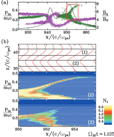
Fig. 2 Ion phase-space plots, x proﬁle of ¯Bz(x), and contour maps ofδBz(=Bz−B¯z) in the (x,z) plane, atΩi0t=0.875.

Fig. 3 (a) Ion phase-space plot and profile of ¯BzatΩi0t=1.125. (b) Expanded view of the front of the right pulse region enclosed by the red line in (a). Magnetic-field lines in the (x,z) plane and ion distributions for different ranges ofz, (1) 38<z/(c/ωpe)<42 and (2) 31<z/(c/ωpe)<35.

interactions with whistler waves [5–7]. The instabilities evolve in the magnetic field that is being gradually com-pressed. Because of the nonlinear evolution of the insta-bilities, 2D fluctuations grow to large amplitudes in the strong magnetic-field pulse region [4]. Figure 2 shows phase-space plots (x,pix) of surrounding ions (green dots)

and exploding ions (pink dots), thexproﬁles of ¯Bzand the contour maps of the 2D ﬂuctuation ofBz,δBz =Bz−Bz,¯ in the (x,z) plane atΩi0t=0.875, which is slightly before

t =tspl. The amplitudes ofδBz are noticeably large near

the position where ¯Bzhas a steep slope and strong current is ﬂowing.

The 2D fluctuations of the electromagnetic fields in-fluence the ion reflection. Figure 3 (a) shows the ion phase space plot and the profile of ¯Bz at Ωi0t = 1.125.

(3)

weak in thezrange (2). The top panel displays magnetic-ﬁeld lines in the (x,z) plane. Magnetic-ﬁeld lines bend forward in range (1) compared to range (2).

The evolution of 2D magnetic ﬂuctuations after t = tspl is rather complex. This is because, in addition to the

complex interactions between surrounding and exploding plasmas, the reflected ions can affect the field structure.

4. Dependence on

v

0

and

θ

We compare the results for the cases ofv0/vA = 12

and 8. Figure 4 displays the contour map of ¯Bzin the (x,t) plane forv0/vA = 8. A strong magnetic-ﬁeld pulse splits

into two atΩi0tspl = 0.85, which is earlier than the time

forv0/vA = 12,Ωi0tspl = 0.95. However, the values of

ΩiEtsplfor the two cases are close. The propagation speeds

of the generated forward and reverse pulses forv0/vA=8

are smaller than those forv0/vA=12, respectively.

Figure 5 (a) shows the evolution of 2D ﬂuctuations of Bzbeforet=tsplforv0/vA=8 and 12. The contour maps

of|δBz|in the (x,t) plane are plotted.|δBz|is deﬁned as

|δBz|(x,t)= 1 Lz

dz|Bz(x,z,t)−Bz(x¯ ,t)|, (3) and the white line shows the positionxmwhere ¯Bz has its

peak value. The 2D ﬂuctuations have large amplitudes in the regionxeb <x<xm; the values of|δBz|forv0/vA=8

are smaller than those forv0/vA=12. Figure 5 (b) shows

the time variations of wavenumber kz for the dominant modes ofδBz. AtΩi0t 0.4,kz forv0/vA =8 is slightly

greater than that forv0/vA =12, which is consistent with

linear theory for modiﬁed two-stream instabilities. As time advances,kzdecreases. This is due to the nonlinear inter-actions of the current ﬁlaments produced by the instabili-ties [4]. The values ofkzfor the twov0’s are close atttspl

for eachv0.

Figure 6 shows the evolution ofδBzaftert =tspl for

the twov0’s. The comparison of Fig. 6 (a) with Figs. 1

and 4 conﬁrms that the amplitudes ofδBzare large in the forward- and reverse-pulse regions. The time variations of wavenumberkzof the dominant modes in the two regions are shown in Fig. 6 (b). This indicates thatkz’s start to de-crease atΩi0t2 for the twov0’s, although there are some

ﬂuctuations. This time is almost equal to the time at which xiEbandxiSbintersect, as shown in Figs. 1 and 4.

In addition tov0/vA =8 and 12, we performed

simu-lations forv0/vA=10, 14, and 16 at ﬁxedθ =90◦.

Fig-ure 7 (a) showsΩiEtspl(black x-mark) as a function ofv0.

Fig. 4 Same as Fig. 1 except forv0/vA=8.

Fig. 5 Evolution ofδBz beforet = tspl forv0/vA = 8 and 12. (a) Contour maps of|δBz|in the (x,t) plane. (b) Time variations of wavenumberkzof dominant mode.

We see thatΩiEtspl ∼ 0.8 for all v0’s. Figure 7 (a) also

shows the Mach numberMfm(≡ |vsh/vfm|) of the generated

forward (red square) and reverse (blue circle) shock waves fromΩi0t =2 to 4, wherevsh is the propagation speed of

a shock wave relative to xeb andvfm is the speed of fast

magnetosonic waves in the upstream region of each shock wave. Asv0increases, the Mfmvalues of the forward and

reverse shock waves also increase.

We plot in Fig. 7 (b) the amplitude of ¯Bz, denoted by Bm, of a strong magnetic ﬁeld pulse at t = tspl (black

x-mark). The amplitudes of the generated forward and re-verse shock waves are also shown; these are values aver-aged over the period fromt =2/Ωi0(>tspl) to 4/Ωi0. The

values ofBmincrease withv0. We also show in Fig. 7 (c)

the magnitude of 2D magnetic fluctuations in a strong magnetic-field pulse att=tspl, whereσBis defined by

σB=

1 ΔxLz

xmax

xmin

dx

Lz

0

dz|B(x,z)−B¯(x)|, (4) whereΔx = xmax−xmin,xmin = xp−25c/ωpeandxmax =

xp+25c/ωpewithxpbeing the position of the pulse. The

value of σB is normalized by Bm. As for 2D

ﬂuctua-tions in the generated forward and reverse shock waves, the time averaged values ofσB/Bmare shown in Fig. 7 (c).

(4)

val-Fig. 6 Evolution ofδBzaftert=tsplforv0/vA =8 and 12. (a) Contour maps of|δBz|. (b) Time variations ofkzof dom-inant mode in the forward pulse region (1) and reverse pulse region (2).

Fig. 7 Dependence onv0. (a) Timetspl (black x-mark). Mach number Mfm’s of the forward (red square) and reverse (blue circle) shock waves fromΩi0t=2 to 4. (b)-(d) The values ofBm, σB, andkz of the dominant mode ofδBz att=tspl(black x-mark) and their averaged values from

Ωi0t=2 to 4 in the forward (red square) and reverse (blue circle) shock waves.

Fig. 8 Dependence onθ. Same as Fig. 7 except thatx-axis isθ.

ues ofσB/Bmin the forward and reverse shock waves are

greater than that in the strong magnetic-ﬁeld pulse. Fig-ure 7 (d) shows the wavenumberkzof the dominant mode ofδBz. Compared tokz of the strong magnetic-ﬁeld pulse att=tspl,kz’s of the forward and reverse shock waves are

small. The dependence ofkzonv0is not so clear.

We next present the results forθ=60◦, 70◦, 80◦, and 90◦at ﬁxedv0/vA =12. Figure 8 shows the same

quan-tities in Fig. 7, except that x-axis is θ. According to the 1D theoretical and simulation study [8], as θ decreases from 90◦, it takes longer for a strong magnetic-ﬁeld pulse to split into two pulses. The 2D simulation, as shown in Fig. 8 (a), conﬁrms this, wheretsplis plotted as a function

ofθ. The amplitudes of ¯Bzand 2D ﬂuctuationσBatt=tspl

are shown in Figs. 8 (b) and 8 (c), indicating that these val-ues are almost constant withθ. The wavenumberskz of the dominant mode ofδBzatt =tspl, which are plotted in

Fig. 8 (d), are roughly estimated asck/ωpe∼0.2 for all the

θ’s. For the generated forward and reverse shock waves, the values ofMfm,Bm,σB, andkzaveraged over the period

aftert=tsplare almost constant withθ.

5. Summary

(5)

Acknowledgement

This work was carried out by the collabora-tion program Grant Nos. NIFS12KNSS036 and NIFS12KNXN246 of the National Institute for Fu-sion Science and by the joint research program of the Solar-Terrestrial Environment Laboratory, Nagoya Uni-versity. It was also supported in part by a Grant-in-Aid

(2013).

[5] N.A. Krall and P.C. Liewer, Phys. Rev. A4, 2094 (1971). [6] J.B. McBride, E. Ott, J.P. Boris and J.H. Orens, Phys.

Flu-ids15, 2367 (1972).

[7] C.S. Wu, Y.M. Zhou, S.T. Tsai, S.C. Guo, D. Winske and K. Papadopoulos, Phys. Fluids26, 1259 (1983).