A Structural Perspective on Disordered Solids

(1)

University of Pennsylvania

ScholarlyCommons

Publicly Accessible Penn Dissertations

1-1-2015

A Structural Perspective on Disordered Solids

Samuel Schoenholz

University of Pennsylvania, [email protected]

Follow this and additional works at:http://repository.upenn.edu/edissertations

Part of theCondensed Matter Physics Commons

This paper is posted at ScholarlyCommons.http://repository.upenn.edu/edissertations/1994 For more information, please [email protected].

Recommended Citation

(2)

A Structural Perspective on Disordered Solids

Abstract

Disordered solids are all around us from glass and plastic to sand and grains. However, compared to their crystalline counterparts, amorphous materials have unusual properties that are relatively poorly understood. A longstanding question is whether or not the unusual behavior of these systems is structural in origin or whether it is purely dynamical in nature. Here we investigate tools to probe the structure of disordered materials and the role that structure plays in determining dynamics. We begin by investigating a particular class of disordered solids called jammed packings which are composed of finitely repulsive spheres. We show that the stability of these systems with respect to continuous perturbations of their boundary is controlled by a structural length scale, known as the transverse length scale, which diverges as the spheres are

decompressed. We then turn to two techniques that are commonly used to measure structural properties of disordered solids in experiment. The first technique, which computes the phonon spectrum from correlations of particle fluctuations, we show can be reliably applied in experiment as long as care is taken that enough data is available for the spectrum to converge. The second technique, which purports to measure local elastic constants, we show to be fundamentally inapplicable to disordered systems, in contrast to the success of the method when applied to crystalline systems. The final sections of the thesis are devoted to examining the role of local structure in determining dynamics in strained glasses and supercooled liquids above the glass transition temperature. We introduce a novel machine learning method for constructing a continuous field, that we call softness, as a coarse graining over local density. We show softness to be more strongly correlated with dynamics than existing methods and demonstrate that it may be applied across a wide range of systems. We leverage the softness picture to show that low temperature glasses under strain can be meaningfully understood in terms of the dynamics of a population of ``soft spots'' in analogy to crystalline systems which are controlled by populations of defects. Finally, we show that the well known heterogeneous dynamics of supercooled liquids arise from a heterogeneous distribution of energy scales in the system, that are in turn correlated with softness. This allows us to construct a simple model for the slow relaxation of glassy liquids that is in excellent agreement with simulation results.

Degree Type

Dissertation

Degree Name

Doctor of Philosophy (PhD)

Graduate Group

Physics & Astronomy

First Advisor

Andrea J. Liu

Keywords

Glass, Jamming, Softness

(3)

Subject Categories

(4)

A STRUCTURAL PERSPECTIVE ON DISORDERED SOLIDS

Samuel S. Schoenholz

A DISSERTATION

in

Physics and Astronomy

Presented to the Faculties of the University of Pennsylvania

in

Partial Fulfillment of the Requirements for the

Degree of Doctor of Philosophy

2015

Andrea J. Liu, Professor of Physics and Astronomy Supervisor of Dissertation

Marija Drndic, Professor of Physics and Astronomy Graduate Group Chairperson

Dissertation Committee

Tom Lubensky, Professor of Physics and Astronomy

Robert Riggleman, Professor of Chemical and Biomolecular Engineering Douglas Durian, Professor of Physics and Astronomy

(5)

A STRUCTURAL PERSPECTIVE ON DISORDERED SOLIDS

COPYRIGHT

Samuel S. Schoenholz

(6)

Acknowledgements

This work, and the five years that this work represents, would not have been possible

without the help of many people. I think that my journey through graduate school

was in large part a process of learning how to approach challenging, open-ended,

problems with no real certainty that a solution existed. I have a lot of people to

thank for helping me develop as a thinker and a scientist.

First and foremost I would like to thank my advisor, Andrea Liu. Andrea is

an outstanding researcher and her rigorous, thoughtful, and insightful approach to

tackling projects has fundamentally shaped my approach to science. She sets a high

bar for when a problem can be considered solved and that pursuit of excellence is

something I aspire to emulate. I really appreciate Andrea’s unrelenting pursuit of

interesting questions. I am also very thankful for the large amounts of freedom

that Andrea has given me over the past five years from choosing which projects to

work on, to providing me with the opportunities to attend conferences and summer

schools, and to letting me spend this coming year at Harvard. Finally, I really

(7)

appreciate her thoughtful advice about life in general.

Next I would love to thank Tom Lubensky, Randall Kamien, and Burt Ovrut for

helping to shape my overall perspective on physics. In particular I think they are

responsible for most of what I know about far too many topics to list here. Thanks

to Tom and Randy in particular for constantly being around to discuss problems

with; both had a large impact my approach to problem solving.

I really enjoyed and appreciated working with Rob Riggleman and J¨org Rottler.

In addition to Andrea, they got me interested in the problem of predicting

rear-rangements in disordered solids using soft spots. I learned a huge amount from both

Rob and J¨org about molecular dynamics simulations. I would also like to thank

Amit Shavit and Anton Smessaert for similar stimulating discussions.

I am thankful for the opportunity to work in collaboration with many great

experimentalists. I think one of the joys of being at Penn was the ease of

collabo-ration between theory and experiment. I really enjoyed working with the group of

Arjun Yodh especially Ke Chen, Tim Still, Ye Xu, and Zoey Davidson. Working

with Jennifer Rieser and Doug Durian on applying our machine learning method to

identify soft spots in their granular pillar was also a pleasure.

I would like to thank Dogus Cubuk for being such a great friend and collaborator

since our first year of college. Dogus really worked hard to get me excited about

(8)

was really born out of conversations between the two of us and generally represent

a joint effort. I’m excited for all the things to come.

The entire soft matter theory group made my time at Penn fun and interesting.

I’d like to thank Carl Goodrich for many great conversations. Especially during my

first few years, talking to Carl really helped me to understand jamming physics.

Working with Carl on my first paper taught me a huge amount about how to play

with data to find patterns. Talking and working with Daniel Sussman was always

fun and informative. I think we share a similar outlook on science and life. I thank

Louis Kang for being a most excellent officemate. I would like to also say that I

really appreciate my interactions with Daniel Beller, Kevin Chiou, Francesca Serra,

Max Lavrentovich, Tom Dodson, Jing Cai, Jason Rocks, and Toen Castle.

I appreciate James Stokes, Zain Saleem, Steven Gubser, and Bogdan Stoica for

getting me interested in spin models in which the target space is compact and

hyperbolic, the results of which are unfortunately absent here.

I’d like to acknowledge the other students in my year who began in the fall of

2010 for making my time (especially the first two years) so enjoyable. In particular

I’d like to say thanks to Alex Tuna and Ben Wieder.

I would like to thank Jenny Marsh for her love and encouragement, inspiring me

to be as good as possible. Lastly I would like to thank my parents, Jace and Ken,

(and my dog) for their constant love, support, and guidance. You made me who I

am today and shaped who I will become.

(9)

ABSTRACT

A STRUCTURAL PERSPECTIVE ON DISORDERED SOLIDS

Samuel S. Schoenholz

Andrea J. Liu

Disordered solids are all around us from glass and plastic to sand and grains.

However, compared to their crystalline counterparts, amorphous materials have

unusual properties that are relatively poorly understood. A longstanding question

is whether or not the unusual behavior of these systems is structural in origin or

whether it is purely dynamical in nature. Here we investigate tools to probe the

structure of disordered materials and the role that structure plays in determining

dynamics. We begin by investigating a particular class of disordered solids called

jammed packings which are composed of finitely repulsive spheres. We show that the

stability of these systems with respect to continuous perturbations of their boundary

is controlled by a structural length scale, known as the transverse length scale, which

diverges as the spheres are decompressed. We then turn to two techniques that are

commonly used to measure structural properties of disordered solids in experiment.

The first technique, which computes the phonon spectrum from correlations of

particle fluctuations, we show can be reliably applied in experiment as long as

care is taken that enough data is available for the spectrum to converge. The

(10)

be fundamentally inapplicable to disordered systems, in contrast to the success of

the method when applied to crystalline systems. The final sections of the thesis

are devoted to examining the role of local structure in determining dynamics in

strained glasses and supercooled liquids above the glass transition temperature.

We introduce a novel machine learning method for constructing a continuous field,

that we call softness, as a coarse graining over local density. We show softness to

be more strongly correlated with dynamics than existing methods and demonstrate

that it may be applied across a wide range of systems. We leverage the softness

picture to show that low temperature glasses under strain can be meaningfully

understood in terms of the dynamics of a population of “soft spots” in analogy to

crystalline systems which are controlled by populations of defects. Finally, we show

that the well known heterogeneous dynamics of supercooled liquids arise from a

heterogeneous distribution of energy scales in the system, that are in turn correlated

with softness. This allows us to construct a simple model for the slow relaxation of

glassy liquids that is in excellent agreement with simulation results.

(11)

List of Tables

6.1 Angular structure function parameters. . . 161

7.1 Number densities and temperatures studied. Each column contains the temperatures studied for a given number densityρ. . . 182

(16)

List of Figures

1.1 The glass transition. (a) The dependence of volume or enthalpy for a glass forming liquid. We see atTm the first-order phase transition to the crystal where the volume changes discontinuously. We also see the volume continuously contract upon further cooling in the super-cooled regime until the system eventually falls out of equilibrium. Ta corresponds to a slowly cooled liquid andTb to a more quickly cooled system. (b) The viscosity (which is proportional to the relaxation time) for several glass forming liquids in the supercooled regime. Here Tg is defined to be when the viscosity reaches 1013 poise. We see that some glass forming liquids behave as ”strong” glass formers with a viscosity that scales arrheniusly while other ”fragile” glass forming liquids scale have viscosities that are super-arrhenius. Both figures are taken from Debeneditti and Stillinger [48]. . . 7

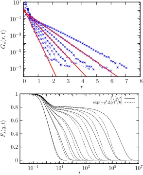
1.2 Relaxation in glassy liquids. (a) The distribution of the van Hove function at increasing time. We see large exponential tails. Taken from Chaudhuri et al.[28]. (b) In solid lines, the self intermediate scattering function as a function of decreasing temperature from high (left) to low (right). In dashed lines we see the naive prediction from simple diffusion. Taken from Berthier [14]. . . 10

1.3 Dynamical heterogeneities. Here we see particles in a two-dimensional glassy liquid colored according to how far they moved, _|ri(t)−ri(0)| from low mobility (blue) to high mobility (red). Each plot shows the mobility after a different amount of time has passed from ta to 50ta wheretais a short timescale related to the length of time for particles to complete a rearrangement. The different populations of particles are apparent. Taken from Keys et al.[80] . . . 12

(17)

1.4 Shear transformation zones. (a) The motion of particles in a sheared glass as measured by D2

min. We note the localized nature of the

rearrangements. (b)-(c) The proposed dynamics of a shear trans-formation zone before and after activation. Taken from Falk and Langer [52]. . . 13

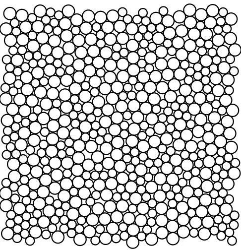
1.5 Jammed packing. Here we show a jammed packing of 512 bidisperse particles with a size ratio of 1:1.4. This packing is at a pressure of 10−4_{. . . .} ₁₆

1.6 Scalings with packing fraction. Here we show numerical results of the scaling of (a) pressure p and (b) shear modulus G for two different choices ofα. Results are shown for packings in two-dimensions (blue) and in red-dimensions (red). . . 17

1.7 (a) The density of states for jammed packings from low density of ∆φ ∼ 10−8 _{(left) to ∆}_φ _∼ ₁₀−2 _{(right) adapted from Liu and}

Nagel [90]. (b) The onset of the plateau in the density of states as a function of ∆φ. Figure adapted from Silbertet al. [121]. . . 25

1.8 The motion of particles along three different vibrational modes from (A) the quasi-localized, (B) the anomalous, and (C) the Anderson localized parts of the spectrum. This figures are also adapted from [90]. 25

1.9 The anharmonic response of jammed packings. (a) shows a plot of the participation ratio for vibrational modes of a jammed packing. We see that modes in the quasi-localized regime are significantly more localized than for modes with ω > ω∗_{. (b) shows a plot of the}

energy barrier to rearrangement in the direction of each mode. We see that quasi-localized modes have anomalously low energy barriers to rearrangement. This figure is also taken from [90]. . . 27

1.10 Soft spots constructed from vibrational modes. (a) shows the popula-tion of soft spots in a 1024 particle packing of harmonic disks at zero temperature. (b) shows the motion of particles during a rearrange-ment overlapping well with one of the soft spots identified. (c) plots the correlation between a single soft spot and a rearrangement as a function of strain before the rearrangement. (d) shows the soft-spot autocorrelation function over time. These figures are taken from [93]. 28

(18)

1.12 The selection of an optimal margin by the SVM. Figure taken from Bishop [17]. . . 34

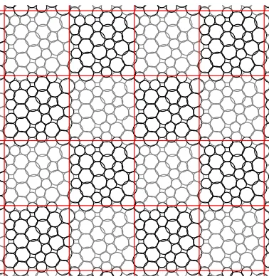
2.1 A 32 particle system with periodic boundary conditions interpreted as a tiling in space. Here a 4_×4 section of the tiling is shown. Shading is used to provide contrast between adjacent copies of the system. . 46

2.2 (a) The dispersion relation for the transverse-acoustic mode (black), longitudinal-acoustic mode (green), and the lowest anomalous mode (red) along the horizontal axis for a system of 128 particles in two di-mensions at a pressure ofp= 10−1_{. The black dashed line shows the}

quadratic approximation to the transverse branch and has a value of λT at the zone edge. The dashed red line shows the flat

approx-imation of the lowest anomalous mode and has a value of λ0. The

system is stable because the lowest branch is never negative. (b) Similar dispersion relations for a system at p = 10−3_{. This system}

has a lattice instability because the lowest mode is negative at large

k. (c)-(d) A 2×4 section of the periodically tiled systems from (a)-(b), respectively. Overlaid are the displacement vectors uiµ for the lowest modes near the zone edge (k ≈0.9π/Lxˆ, see the blue dot in (a)-(b)). Note that the mode in (c) is stable (λ >0) and has strong transverse plane-wave character, while the mode in (d) is unstable (λ <0) and has strong anomalous character. . . 51

2.3 Dispersion relations along the Γ₋M line for the lowest few branches of 2 different 2-dimensional packings of N = 1024 particles. The Γ point is at the Brillouin zone center (k = 0) and the M point is at the zone corner where the magnitude of k is greatest. (a) A “shear-unstable” packing (i.e. a sphere packing that is unstable at low k) atp= 10−4 _{(black) and the dispersion relation for the corresponding}

unstressed system (blue). (b) A “lattice-unstable” sphere packing (i.e. a packing that is stable near k= 0 but is unstable at higher k) atp= 10−4 _{(black) and the dispersion relation for the corresponding}

unstressed system (blue). (c) Comparison between the lowest branch in the sphere packing (black) and its unstressed counterpart (blue) for the same system as in (b). The dashed magenta line is the difference between the two eigenvalue branches. . . 52

(19)

2.4 The average eigenvalue of the lowest mode at the corner of the Bril-louin zone of the unstressed system (blue), as well as the average difference between the unstressed system and the original packing (magenta), in (a) two and (b) three dimensions. The blue and ma-genta data exhibit collapse as predicted by eqns (2.4.4) and (2.5.1), with the caveat that we were unable to reach the low pressure regime in three dimensions where we expect the scaling to be different. Data is only shown when at least 20 shear stable configurations were ob-tained. . . 56

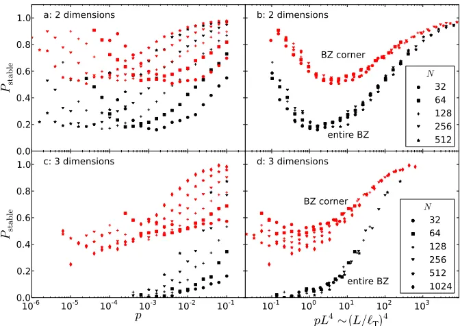
2.5 The fraction of shear-stable systems in two and three dimensions that are also k >0-stable. In red we plot the fraction of systems that are unstable at theM point while in black we plot the fraction of systems that are stable everywhere. We see that both collapse with pL4_{, or}

equivalently L/`T, with the expected exception of the low pressure

regime in three dimensions. . . 58

3.1 Distribution of instantanious projection coefficient cω(t) for a. the lowest frequency mode, mode 0; and b. the 10th lowest frequency mode. Red lines are Gaussian fits to the distributions. . . 68

3.2 Phonon modes in 2D colloidal crystals. a. Accumulated mode num-ber, N(ω), as a function of frequency, for a nearly perfect crystal (blue squares) and an imperfect one (red square); ω2 _{is drawn for}

comparison (black line), small arrows points to the modes whose real space vector distributions are plotted in b and c. b, c. Spatial distribution of a low-frequency mode for the b nearly perfect and c imperfect crystal; the direction and magnitude of polarization vectors are represented by the direction and size of the arrows. . . 69

(20)

3.4 Correction for limited number of frames. a. Linear dependence of eigenfrequencies onN/T from simulation. n is the mode index that increases from low to high frequencies. For better visualisation, a constant has been substracted for each curve. b. Linear convergence of eigenfrequencies from experimental data with N/T. The frequen-cies are subtracted by the frequency from the full length of the video,

ωf ull. c. Density of states for different ratios of N/T from simulation. 75

3.5 Correction for limited field of veiw. a. Dispersion curves along differ-ent directions from uncorrected data. Circles represdiffer-ent longitudinal modes and crosses represent transverse modes. Directions are in-dexed in the basic vectors of the reciprocal lattice. b. Dispersion curves along different directions after Hann window function correc-tion. . . 77

3.6 Low frequency modes in a colloidal crystal with defects.a. A snap-shot of an imperfect PNIPAM crystal with a grain boundary in the middle of the field of view, the scale bar is 10 µm. b. Participation ratio for eigenmodes in crystal with defects. c. Color contour plots indicate polarization magnitudes for each particle, summed over the low frequency modes with participation ratio less than 0.2. Circles indicate ”defect” particles identified by local structural parameters. 77

4.1 Probability distribution ofLd_Λ2

xy for simulations ind= 2 (upper red circles) and d = 3 (lower blue circles) of harmonic repulsive spheres atT = 10−5_{. Curves are best-fit}_χ2 _{distributions. Inset: Probability}

distribution of the unscaled Λ2

xy for the experimental colloidal system. 89

4.2 Collapsed probability distributions ofP(Λxx) (blue points) andP(Λxy) (red points) as computed for ∆t= 2τ. (A) Scaling collapse ofP(Λαβ) for 2D simulations with√T for coarse-graining scaleL= 2,p= 10−2

and temperatures of T = 10−5_, ₂_×₁₀−5_, ₄_×₁₀−5_, ₆_×₁₀−5_, ₈_×

10−5_, ₁₀−4_{. Dashed line is the prediction from Appendix 4.6.2. (B)}

Scaling collapse of P(Λαβ) for 2D simulations with L2 forT = 10−5,

p= 10−2_{, and}_L_{= 2}_, ₄_, ₆_, ₈_, ₁₀_, ₁₂_, _{14. Dashed line is the}

predic-tion from Appendix 4.6.2 for theL= 6 data set. (C) Scaling collapse of P(Λαβ) for 3D simulations with L2.5 for T = 10−5, p= 10−2, and

L= 2, 4, 6, 8, 10, 12, 14. . . 92

(21)

4.3 Inverse variance of Λxx (blue circles) and individual particle displace-ment magnitude (red squares) for 2D simulations withT = 10−5 _and

L= 4 as a function of pressure, normalized by the value atp= 10−4_.

Dashed line is the predicted scaling of the bulk modulus with pres-sure. Inset: Ratio of the variance of the diagonal to off-diagonal component of Λαβ as a function of pressure. The corresponding ratio of moduli scales asG/B _∼√p (dashed line). . . 94

4.4 (A)P(Λxx) (red-to-orange color scale) andP(Λxy) (dark-to-light blue color scale) for 2D simulation data with p = 10−2_, _T _{= 10}−5_, _L_{= 4}

for ∆t/τ = 2, 10, 20, 50, 100, 200. Data sets with smaller variance correspond to shorter ∆t. (B)P(Λ2

xy) normalized by the variance for the above ∆t (red points correspond to the shortest ∆t, light blue points to the longest ∆t). Dark blue open circles are experimen-tal data. The solid curve shows a unit-variance χ2 _{function, which}

matches the short-time data very well. . . 96

4.5 (A) Inverse variance of P(Λxx) as a function of ∆t for pressures be-tweenp= 10−2 _{(blue, upper curve) and}_p_{= 10}−4 _{(red, lower curve).}

Inset: Ratio of the variance of the diagonal to the off-diagonal com-ponents of Λαβ as a function of ∆t (B) Ratio of variance of diag-onal and off-diagdiag-onal components of Λαβ as a function of pressure for ∆t/τ = 2,20,200. The corresponding ratio of moduli scales as

G/B _∼√p. . . 97

4.6 var[Λxx+Λyy], as a function of coarse graining sizeLin the simulation of two-dimensional harmonic disks for pressures fromp= 10−2 _(blue,

bottom lines) to p = 10−3.4 _{(red, top lines). Overlaid in black is a}

line with slope −3. Here Λαβ was calculated with ∆t = 5× 104, deep into the caged regime. Inset: var[Λxx + Λyy] as a function of coarse-graining scale (measured in microns) for area fractions φ = 0.8625,0.8695,0.8822 (top to bottom). . . 98

4.7 Mean-squared displacement (in units of particle diameters) for p = 10−3.4_, ₁₀−3.0_, ₁₀−2.4_, ₁₀−2.0 _{(top to bottom). Inset. Mean-squared}

(22)

4.8 Normalized probability distributions of (Λxx+ Λyy)−2 for the exper-imental colloidal system at a fixed volume fraction, truncated to a fixed dynamical range, for several different choices of the box coarse graining size. The fits are exponential decays, and the curves are cal-culated distributions for L = 1,3,4,11,20 microns. Inset. Inferred modulus from the exponential decay fits normalized by the measured value by the methods in Ref. [127] as function of L. Data sets are for φ= 0.8625,0.865,0.8695,0.8775,0.8822. . . 116

5.1 An example configuration of the system at T = 0.1 and ˙γ = 10−4_.

Particles are colored according to their D2

min value (see text).

Par-ticles outlined in black are members of the soft-spots for this con-figuration. The soft-spots have been generated usingNm = 430 and

Np = 20. Inset: a single soft spot coinciding with a rearrangement. . 121

5.2 The probability of a particle residing in a soft-spot as a function of its D2

min value. (a) shows a comparison of the temperatures studied

from T = 0.1 in blue to T = 0.4 in red at a strain rate of ˙γ = 10−4

and (b) shows a comparison of strain rates studied from ˙γ = 10−5

in dark blue to ˙γ = 10−3 _{in green at a temperature of} _T _{= 0}_._1.

In all cases we see that the probability increases with D2

min until

some threshold D2

th ' 15T (vertical dashed line) at which point the

probability reaches some plateau value P∗_{. The soft spot density,} ρSS, is marked by a horizontal dashed line. . . 124

5.3 The difference in probability, ∆P∗ ₌_P∗₍_T,_γ_˙₎₋_ρ

SS, as a function of

Nm and Np for a temperature of T = 0.1 and strain rate ˙γ = 10−4. We see a broad plateau over which ∆P∗ is largely independent ofNm and Np with a weak maximum occurring at Nm? = 430 and Np? = 20 (marked by a star.) The behavior of ∆P∗ is largely independent of temperature and strain rate. . . 126

5.4 The plateau probability,P∗_{, for a particle with high}_D2

minto reside in

a soft spot, normalized by the soft spot density,PSS. This represents how much more likely rearrangements are to be found at soft spots than if the soft spot map were completely uncorrelated with rear-rangements. A value of 1 (dashed line) represents the uncorrelated value. The ratio is 0 when the soft spot map is anti-correlated and so describes no plastic activity. The value of 5.2 represents maximum possible value ofP∗_{, 1}_/ρ

SS, which occurs if all of the plastic activity resides in soft spots. Data is shown for strain rates ˙γ = 10−5 _{in dark}

blue to ˙γ = 10−3 _{in green. . . 127}

(23)

5.5 Correlation functions of theD2

min field and the soft-spot population.

On the left are comparisons of the temperatures considered from blue for T = 0.1 to red for T = 0.4 at a strain rate of ˙γ = 10−4_{. In the}

middle column are comparisons of the strain rates considered from dark blue for ˙γ = 10−5 _{to green for ˙}_γ _{= 10}−3 _{scaled by the strain}

rate, t/τ _→ γt˙ at a temperature T = 0.1. On the right are com-parisons of the strain rates considered from brown for ˙γ = 10−5 _to

yellow for ˙γ = 10−3 _{scaled by the strain rate,} _t/τ _→_γt_˙ _{at a}

temper-ature T = 0.4. Figures (a)-(c) show the self-intermediate scattering function,F(qmax, t), evaluated atq= 2π/σAAyˆ. Figures (d)-(f) show the autocorrelation function for D2

min. Figures (g)-(i) show the

au-tocorrelation function for the soft spot population. In (g) at each temperature comparisons are made with the cumulative probability density function for individual soft spot lifetimes, introduced in sec-tion V, overlaid in dashed lines. In (h) a single comparison is made to

P(τL≥δt), shown using a dashed black line, for lifetimes aggregated from lifetimes collected at all three different strain rates. In (i) predic-tions from the cumulative probability density function for individual soft spot lifetimes are shown for the two faster strain rates overlaid in dashed line. Figures (j)-(l) show the cross correlation between D2

min

and the soft spot population. The plots in both the middle and left columns feature two vertical dashed lines to serve as guides to the eye. The earlier line occurs at a time, τ∗_{, when the self-intermediate}

scattering function first drops below the plateau. The later line oc-curs at the relaxation time, τα, defined so that F(qmax, τα)∼e−1. . 130 5.6 (a)-(c) Probability distributions for single-soft-spot lifetimes at

differ-ent temperatures and strain rates respectively. In (a) temperatures of T = 0.1 (blue) to T = 0.4 (red) are shown at a strain rate of

˙

γ = 10−4_{. Overlaid in dashed lines are the predictions of the}

dis-crete model. In (b) we show lifetime distributions at strain rates of ˙γ = 10−5 _{(dark blue) to ˙}_γ _{= 10}−3 _{(green) at a temperature of}

T = 0.1. Again, predictions from the discrete model are shown in dashed lines using for strain rates of ˙γ = 10−4 _{and ˙}_γ _{= 10}−3_{. In (c)}

we show lifetime distributions at strain rates of ˙γ = 10−5 _{(brown) to}

˙

γ = 10−3 _{(yellow) at a temperature of} _T _{= 0}_._{4. Predictions from the}

(24)

6.1 Snapshot configurations of the two systems studied. Particles are colored gray to red according to theirD2

minvalue. Particles identified

as soft by the SVM are outlined in black. (a) A snapshot of the pillar system. Compression occurs in the direction indicated. (b) A snapshot of thed= 2 sheared, thermal Lennard-Jones system. . . . 151

6.2 Probability that a particle of a givenD2

min value is soft. The vertical

dashed lines are corresponding D2

min,0 values. (a) The result for the

pillar system, wheredAA refers to the large grain diameter (since this is a granular system with macroscopic grains, thermal fluctuations are negligible). (b) The result of using an SVM trained at a tem-perature T (T = 0.1,0.2,0.3 and 0.4 shown in different colors ) to classify data at the same temperature for the d = 2 LJ glass. (c,d) Results for species A and B, respectively, for the d = 3 system at

T = 0.4,0.5 and 0.6. . . 154

6.3 Radial distribution functions averaged over hard (black lines) or soft (red lines) particles. gAB and gBA of soft particles are not equal to each other since they refer to different kinds of regions: neighbors of soft particles from species A and neighbors of soft particles from species B, respectively. . . 156

6.4 (a) Distribution ofGA

B(i;rABpeak), proportional to the gaussian weighted

density at rAB

peak, for soft (red) and hard (blue/green) particles. rpeakAB

corresponds to the first peak of gAB or gBA. (b) Distribution of ΨB

AB(i; 2.07σAA,1,2), proportional to the density of neighbors with small bond angles near a particlei, for soft (red) and hard (blue/green) particles. The inset shows examples of configurations with corre-sponding radial and bond orientation properties, where dark (light) gray neighbors are of species A (B). . . 157

6.5 Identification accuracy over all hard and soft particles in the test set, as a function of D2

min,0 in units ofσAA. . . 162 6.6 Comparison of soft particles computed using local structures (black)

and low-frequency vibrational modes (red) for the Lennard-Jones sys-tem atT = 0.1. . . 165

(25)

6.7 A quantitative comparison of soft particles identified using the SVM method with those identified using the low-frequency vibrational modes of the inherent structure (QLM method). In all plots the color indicates temperature with blue atT = 0.1 and red at T = 0.4. (a) shows the self intermediate scattering function,Fs(q, t) as a func-tion of time whereq =qmaxis the wavevector at the first peak ofS(q).

(b) shows the autocorrelation of QLM soft particles, identified from low-frequency vibrational modes. (c) shows the cross-correlation be-tween soft particles identified using the QLM and SVM methods. (d) shows the autocorrelation of SVM soft particles identified from local structures. We see that all curves are qualitatively similar and decay to zero at approximately the same time. . . 166

6.8 Probability that a particle of a givenD2

min value is soft. Here the soft

particles are classified (in other words, the SVM is trained) using the inherent structures of the configuration. The vertical dashed line is D2

min,0. Here we show that as temperature increases the

predic-tive power of the SVM degrades. This is contrasted with an SVM trained on thermal configurations, whose prediction accuracy does not depend on temperature. . . 167

6.9 (a) Probability that a particle of a given D2

min value is soft. The

vertical dashed line is Dmin,02 . Here we show the result of using an

SVM trained at T = 0.4 to classify data at all temperatures. (b) Same as (a) but with D2

min is scaled by corresponding T. . . 168

6.10 Fraction of misclassified soft and hard particles at different C values. 170

6.11 Classification accuracy on the training and the test set as a function of training set size. . . 171

(26)

7.2 The relationship between softness and dynamics. (a) The probabil-ity that particles rearrange as a function of their softness, PR(S), for temperatures T =0.47, 0.53, and 0.58 plotted in blue to red. Solid lines are measurements from molecular dynamics trajectories (solid lines). Dashed lines present the probability computed using the Arrhenius form for PR(S) (dashed lines). Points represent the probabilities calculated from the zero-time derivative of the over-lap, ₋dq(S, t)/dt at T = 0.47 and T = 0.58. (b) PR(S) as a function of 1/T for 5 different softness values from S _{∼ −}3 (blue) to S _∼ 3 (red). The inset shows the collapse of these probabili-ties when PR/P0 is plotted against ∆E/T. (c) ∆E and Σ, where

PR(S) = exp(Σ−∆E/T), vs. softness S. (d) predicted onset tem-peratureT0 vs.T0m, onset temperature measured by Keys, et al. [80],

for densities ρ = 1.15,1.20,1.25,1.30. The straight line corresponds toT0 =T0m. . . 177

7.3 Overlap calculated from softness a, Solids lines are the measured overlap function, for temperatures T = 0.45, 0.47, 0.53, 0.58, 0.63, and 0.70, from blue to red, respectively. The dashed lines in the insets show predictions assuming each Arrhenius process is independent of one another. (b), The solid lines in the insets are the same as in (a). Dashed lines are predictions for the overlap function from PR(S) including changes in the softness field induced by spatial correlation between rearranging particles. . . 178

7.4 Time evolution of softness. (a) The stochastic evolution of softness in time as seen in through the evolution of the Gaussian approximation to the distribution of softness. (b) The time evolution of the softness distribution for a collection of particles with initial softness S0 ∼ −3

from t = 0 (blue) to t = 1000τ (pink). Points are the measured histogram values, and the dashed lines are Gaussian approximations to the distribution. (c) The time evolution of the average softness for particles that start from several softness values ranging fromS0 ∼ −3

(blue) to S0 ∼3 (red). . . 180

7.5 The typical trajectory of a particle at T = 0.47 and ρ = 1.20. (a) The values of phop over the course of the timeseries that contains

three events. (b) The distance the particle has moved from its initial position over time. In green and red dashed lines indicate the begin-ning and end, respectively, of the events that we identify. Notice the clear separation of scales between events and the rest of the trajectory.187

(27)

7.6 The characteristic size and timescale of events (potential rearrange-ments). (a) The distribution of displacements experienced by par-ticles during rearrangements with p∗_hop ≈ 0.05, 0.15, 0.25, and 0.35 at T = 0.47 from black to red respectively. (b) The distribution of durations of displacements observed at the same values ofp∗_hop as in (a). . . 187

7.7 The average size and timescale of events. (a) The average size of events as a function of p∗

hop at temperatures T = 0.45, 0.47, 0.51,

0.53, 0.56, 0.58, 0.63, 0.70 from blue to red respectively. The average durations of events for the same temperatures as in (a). . . 188

7.8 The fraction of rearranging particles that were correctly identified as soft as a function of pcat T = 0.47 andρ= 1.20. A line guiding the eye is drawn atp∗

hop = 0.2. . . 189

7.9 The dependence of the energy and entropy scales on the cutoff pc. (a) The energy scale as extracted from the Arrhenius form for rear-rangements with cutoffs pc =0.05, 0.08, 0.11, 0.14, 0.17, 0.20, 0.23, 0.26, 0.29, 0.32 from black (lowest) to red (highest). (b) The entropy scale for the same cutoffs as in (a). . . 190

7.10 The shift in the energy scale as a function of the logarithm of the cutoff. . . 191

7.11 (a) The degree of directional correlation between displacements dur-ing a rearrangement and the gradient of the softness field. (b) The PDF of cosθ for increasing values of _|∆r_||∇S_| from low (blue) to high (red). . . 192

7.12 The deviation of the energy scale ∆E(S) from linear behavior in S

atT = 0.47 and ρ= 1.20. . . 193

7.13 The fraction of rearrangements that are irreversible, firrev (a) as a function of softness for temperatures from T = 0.47 (blue) to T = 0.63 (red); (b) as a function of temperature. . . 194

(28)

7.15 The changing softness distribution with temperature. (a) The distri-bution of softness at different temperatures from T = 0.47 (blue) to

T = 0.70 (red). (b) The changes in the mean softness over this range as a function of 1/T. Overlaid in dashed line is a fit toµS(T)∼1/T2.199 7.16 The non-exponential decay of overlap. (a) the softness-dependent

overlap q(S, t) for two representative temperatures T = 0.47 (long time) andT = 0.58 (short time) at four softnesses from₋4 (blue) to 4 (red). (b) the average overlap at all temperatures from T = 0.45 (blue) to T = 0.70 (red). . . 199

7.17 The propagator for the directed diffusion process at different times from t = e−6 _{(blue) to} _t ₌ _e _{(red). The parameters used here are}

S0 = 1, µS = 0, and θ= 1. . . 202 7.18 The measured variance of the softness propagator at T = 0.45 (blue)

vs the result of directional diffusion with θ fit. . . 203

7.19 The measured variance of the softness propagator (blue) against the result of directional diffusion withθ fit (dashed black) including the thermal fluctuation term. From top left in a ”z” shape we have

T = 0.45 at low softness, T = 0.58 at medium softness, T = 0.51 at low softness, and T = 0.51 at high softness. . . 204

7.20 The measured mean of the softness propagator (colored) against the result of directional diffusion withθ fit (dashed black) from low soft-ness (blue) to high softsoft-ness (red). From top left in a ”z” shape we haveT = 0.45, 0.47, 0.51, 0.56. . . 205

7.21 Cross-validation accuracy as a function of γ and C. . . 207

7.22 Black curves represent the classification accuracy of the SVM trained on a radial structure function at r. Red curves are the radial distri-bution function of neighbors of the given type. . . 210

7.23 The accuracy of an SVM trained on a pair of radial structure func-tions. The axes denote type / distance of the structure functions used and the color denotes the resulting cross-validation accuracy. 211

7.24 Black curves denote the number of high accuracy triplets a radial structure function was in. Red curves denote the radial distribution function in arbitrary units. . . 212

(29)

7.25 Best accuracy achieved for a given number of radial structure func-tions. The dashed lines represent the accuracy achieved by using all 100 radial structure functions. . . 213

(30)

Chapter 1 Introduction

The last century has seen unprecedented progress in our understanding of nature.

The collective behavior of large numbers of particles has been codified into the

fields of statistical physics and condensed matter physics. In turn these subjects

successfully tackled many longstanding mysteries about the world around us. The

ubiquity of phase transitions across many disparate systems was understood first

in terms of Landau’s insight that the nature of critical points depends only on the

symmetries of the system and then later by Kadanoff, Wilson, and Fisher in terms

of renormalization group fixed points and irrelevant operators. A second key insight

has been the realization that the behavior of materials is frequently controlled by a

small population of defects rather than by the bulk. Consequently, theories based on

populations of defects have been used to understand why the yield stress of crystals

is orders of magnitude lower than naive predictions from continuum elasticity, why

(31)

solids harden upon being annealed, and the mechanism for melting in a host of

different systems.

This striking progress in science is inexorably linked to a similarly rapid

explo-sion of technology. While science and technology are not always directly linked

there are countless examples of advances in our understanding of nature that have

far reaching implications for our daily lives. The success of band theory aided the

development of semiconductors that form the backbone of modern electronics.

Si-multaneously, work on the mechanical properties of solids has led to stronger and

lighter materials. Looking to the future, a much sought after theory of high

tem-perature superconductivity offers tantalizing possibilities for transferring power and

data across large distances.

Amidst all of this improvement, our understanding of disordered solids and

glasses has progressed more modestly. The non-equilibrium nature of these

sys-tems coupled with a lack of positional order of the constituent particles has stymied

a theoretical understanding of amorphous materials. To date a slew of fundamental

questions remain about the nature of disordered materials. It is unknown whether

there is a phase transition between a liquid and a glass or whether glasses are very

sluggish fluids. Moreover, the question of whether the behavior of these systems is

controlled by a population of defects - in analogy to the crystalline case - remains

highly contentious. Unlike in the case of crystals, the lack of order amongst the

(32)

material that look different from the bulk. Answering these questions might allow

us to understand many aspects of disordered solids - such as failure, melting, and

the trade off between strength and toughness - that are of broad theoretical and

practical interest. Recall that the recent ubiquity of smartphones and tablets has

relied heavily on the use of stronger scratch resistant glass.

These advances in science and technology have grown hand in hand with new

tools to probe more deeply into the world around us. Chief among these new

advances are a diverse set of methods, leveraging ever more powerful computers,

that allow us to access the trajectories of individual atoms across a diverse set

of systems. Simulations of particles with nearly arbitrary interactions can tackle

increasingly large systems for ever increasing amounts of time. In experiment,

video microscopy and particle tracking allows us to track a similarly large number

of particles in colloidal and granular real atom systems. However, the power of

these techniques also brings about new challenges in analyzing these systems due to

the vast amounts of data they generate. Since much of the machinery of statistical

mechanics is developed to study bulk properties, can access to individual particle

trajectories offer any qualitative advantage over typical scattering experiments?

Moreover, in experimental systems where the Hamiltonian of the system is often

obscured, what kinds of statements can be made from particle trajectories alone?

In the face of questions like these, we notice that since the 1990’s the field of

ma-chine learning has seen burgeoning success on the back of increasingly large datasets.

(33)

Machine learning formalizes statistical methods for regression and classification on

large datasets, and plays a critical role across modern technology in applications

such as predictive searching on google and speech-to-text translation. These

tech-niques have recently found use in physics. At CERN neural networks have been

used to identify and reconstruct interesting events amongst the petabytes of data

produced in particle collisions. In condensed matter physics, Behler and

collabo-rators [12] used similar techniques to find empirical potentials for Silicon systems

that were both extremely fast and accurate. However, the uses of machine learning

in physics have typically been limited to regression and classification. Is it possible

to use these methods to gain conceptual understanding of a complex system or to

formulate an effective theory of a complex phenomenon?

The principal purpose of this thesis will be to argue that the behavior of

dis-ordered solids and glassy liquids can be meaningfully understood in terms of local

structures that are akin to defects in crystals. We use machine learning methods

to identify a coarse graining of local degrees of freedom to a single scalar field

-called softness - that most strongly correlates with dynamics. We then use this

scalar field to show that the mysterious process of relaxation in glassy liquids can

be understood in terms of a theory based on softness. This technique appropriately

leverages the large quantities of data available in experiment and simulations and

-we believe - may be used to tackle many outstanding questions about the behavior

disordered solids. To our knowledge this represents the first use of machine learning

(34)

This work draws inspiration from Manning and Liu [93] who showed that a

population of defects, called “soft spots”, could be identified in a special class

of disordered systems called “jammed” solids by considering low-frequency

quasi-localized vibrational modes. We show that this formalism can describe the plasticity

of a strained glass in two-dimensions at relatively low temperatures and high strain

rates. Moreover, we show that the rate of relaxation of defects in the system can be

understood in terms of the dynamics of individual defects. However, the correlation

between plasticity and the soft spots identified in this way is rather weak even at

low temperatures and is expected to deteriorate at higher temperatures and in

three-dimensions.

A secondary goal of this thesis is to investigate what properties of an

experimen-tal system may be determined from particle trajectories alone. In our work using

machine learning to identify defects, we show that our technique may be applied to

wide range of experimental systems. This includes disordered solids composed of

grains where the presence of friction means that a description in terms of a

hamil-tonian might be inappropriate. We also study a commonly used method of using

particle level fluctuations to identify the vibrational spectrum and elastic moduli

of disordered packings of colloids. While these methods generally succeed, we show

that great care must be taken that enough independent data is available since the

modes tend to converge as N/T where N is the number of degrees of freedom and

T is the number of independent frames used in the analysis. Finally, we consider

another commonly used method for finding the elastic moduli based on particle

(35)

level fluctuations and show that - while other results indicate that the method can

be successfully applied to crystalline systems - this method is fundamentally flawed

when applied to disordered systems.

1.1 The glass transition

All around us liquids freeze to solids upon cooling. In many cases this process is

achieved via a first order phase transition. In this case, at a critical temperature,

Tm, the free energy of the disordered, isotropic, and homogeneous arrangement of

particles in the fluid becomes equal to the free energy of the ordered anisotropy

of the crystalline phase. The ordered phase proceeds to nucleate in the fluid until

- upon further cooling - the crystal dominates the fluid. In the view of Landau

this process is relatively well understood and is described by the breaking of the

continuous rotational and translational symmetries of the fluid down to the discrete

set of crystallographic symmetries.

However, the process of nucleation is frequently slow. Therefore, if the liquid

is cooled quickly enough crystallization can be avoided and the system enters a

long-lived metastable state known as the supercooled liquid. As the temperature

of the supercooled liquid is lowered further it becomes increasingly sluggish. At

some temperature, known as the glass transition temperatureTg, the time required

(36)

insight

review articles

NATURE|VOL 410|8 MARCH 2001|www.nature.com 261

response to an imposed deformation) can often be described by the stretched exponential, or Kohlrausch–Williams–Watts (KWW) function26,27

F(t)!exp["(t/#)$_{] (}_$_{< 1)} ₍₂₎

where F(t)![%(t)"%(&)]/[%(0)"%(&)] and %is the measured quantity (for example, the instantaneous stress following a step change in deformation). #in equation (2) is a characteristic relax-ation time, whose temperature dependence is often non-Arrhenius (exhibiting fragile behaviour). The slowing down of long-time relaxation embodied in equation (2) contrasts with the behaviour of liquids above the melting point, which is characterized by simple exponential relaxation. Experimental and computational evidence indicates that this slow-down is related to the growth of distinct relaxing domains28–39_{(spatial heterogeneity). Whether each of these}

spatially heterogeneous domains relaxes exponentially or not is a matter of considerable current interest38,39_.

Decouplings

In supercooled liquids below approximately 1.2Tg there occurs a

decoupling between translational diffusion and viscosity, and between rotational and translational diffusion30,39,40_{. At higher}

temperatures, both the translational and the rotational diffusion coefficients are inversely proportional to the viscosity, in agreement with the Stokes–Einstein and Debye equations, respectively. Below approximately 1.2Tg, the inverse relationship between translational

motion and viscosity breaks down, whereas that between rotational motion and viscosity does not. Near Tg, it is found that molecules

translate faster than expected based on their viscosity, by as much as two orders of magnitude. This therefore means that, as the temperature is lowered, molecules on average translate progressively more for every rotation they execute. Yet another decoupling occurs in the moderately supercooled range. At sufficiently high temperature the liquid shows a single peak relaxation frequency (Fig. 3), indicative of one relaxation mechanism. In the moderately supercooled regime, however, the peak splits into slow (') and fast ($) relaxations41–43_{. The former exhibit non-Arrhenius behaviour}

and disappear at Tg; the latter continue below Tg and display

Arrhenius behaviour44_.

Thermodynamics

The entropy of a liquid at its melting temperature is higher than that of the corresponding crystal. Because the heat capacity of a liquid is higher than that of the crystal, this entropy difference decreases upon supercooling (Box 1). Figure 4 shows the temperature dependence of the entropy difference between several supercooled liquids and their stable crystals45_{. For lactic acid this entropic surplus is consumed so}

fast that a modest extrapolation of experimental data predicts its impending vanishing. In practice, the glass transition intervenes, and

(Sdoes not vanish. If the glass transition did not intervene, the liquid entropy would equal the crystal’s entropy at a nonzero temperature

TK(the Kauzmann temperature.) Because the entropy of the crystal

approaches zero as Ttends to zero, the entropy of the liquid would eventually become negative upon cooling if this trend were to contin-ue. Because entropy is an inherently non-negative quantity (Box 1), the state of affairs to which liquids such as lactic acid are tending when the glass transition intervenes is an entropy crisis46–48_{. The}

extrapola-tion needed to provoke conflict with the third law is quite modest for many fragile liquids49_{, and the imminent crisis is thwarted by a}

kinetic phenomenon, the glass transition. This suggests a connection between the kinetics and the thermodynamics of glasses47_{. The}

thermodynamic viewpoint that emerges from this analysis50

considers the laboratory glass transition as a kinetically controlled manifestation of an underlying thermodynamic transition to an ideal glass with a unique configuration.

A formula of Adam and Gibbs51_{provides a suggestive connection}

between kinetics and thermodynamics:

t!Aexp(B/T sc) (3)

In this equation, tis a relaxation time (or, equivalently, the viscosity) and Aand Bare constants. sc, the configurational entropy, is related to

the number of minima of the system’s multidimensional potential energy surface (Box 2). According to the Adam–Gibbs picture, the origin of viscous slow-down close to Tgis the decrease in the number

of configurations that the system is able to sample. At the Kauzmann temperature the liquid would have attained a unique, non-crystalline state of lowest energy, the ideal glass. Because there is no configura-tional entropy associated with confinement in such a state, the Adam–Gibbs theory predicts structural arrest to occur at TK. In their

derivation of equation (3), Adam and Gibbs invoked the concept of a cooperatively rearranging region (CRR)51_{. A weakness of their}

treatment is the fact that it provides no information on the size of such regions. The fact that the CRRs are indistinguishable from each other is also problematic, in light of the heterogeneity that is believed to underlie stretched exponential behaviour8_.

Figure 1Temperature dependence of a liquid’s volume v or enthalpy h at constant pressure. Tmis the

melting temperature. A slow cooling rate produces a glass transition at Tga; a

faster cooling rate leads to a glass transition at Tgb.

The thermal expansion coefficient

'p!()lnv/)T )pand

the isobaric heat capacity cp!()h/)T )pchange abruptly but continuously at Tg.

Tm Volume, Enthalpy Liquid Glass Crystal a b

TemperatureTgaTgb

Figure 2Tg-scaled Arrhenius representation of liquid viscosities showing Angell’s

strong–fragile pattern. Strong liquids exhibit approximate linearity (Arrhenius behaviour), indicative of a temperature-independent activation energy

E!dln*/d(1/T ) ≈const. Fragile liquids exhibit super-Arrhenius behaviour, their effective activation energy increasing as temperature decreases. (Adapted from refs 9 and 11.)

14 12 10 8 6 4 2 0 -2 -4

Log (viscosity in poise)

Fragile

Strong

m,o-Fluorotoluene

Chlorobenzene Toluene

m,o-Xylene

o-Terphenyl

K + Bi3+

CI-SiO₂

GeO₂

K+_Ca2+_NO

3

-Tg/T

insight

review articles

NATURE|VOL 410|8 MARCH 2001|www.nature.com 261 response to an imposed deformation) can often be described by the

stretched exponential, or Kohlrausch–Williams–Watts (KWW) function26,27

F(t)!exp["(t/#)$_{] (}_$_{< 1)} ₍₂₎

where F(t)![%(t)"%(&)]/[%(0)"%(&)] and %is the measured quantity (for example, the instantaneous stress following a step change in deformation). #in equation (2) is a characteristic relax-ation time, whose temperature dependence is often non-Arrhenius (exhibiting fragile behaviour). The slowing down of long-time relaxation embodied in equation (2) contrasts with the behaviour of liquids above the melting point, which is characterized by simple exponential relaxation. Experimental and computational evidence indicates that this slow-down is related to the growth of distinct relaxing domains28–39_{(spatial heterogeneity). Whether each of these}

spatially heterogeneous domains relaxes exponentially or not is a matter of considerable current interest38,39_.

Decouplings

In supercooled liquids below approximately 1.2Tgthere occurs a

decoupling between translational diffusion and viscosity, and between rotational and translational diffusion30,39,40_{. At higher}

temperatures, both the translational and the rotational diffusion coefficients are inversely proportional to the viscosity, in agreement with the Stokes–Einstein and Debye equations, respectively. Below approximately 1.2Tg, the inverse relationship between translational

motion and viscosity breaks down, whereas that between rotational motion and viscosity does not. Near Tg, it is found that molecules

translate faster than expected based on their viscosity, by as much as two orders of magnitude. This therefore means that, as the temperature is lowered, molecules on average translate progressively more for every rotation they execute. Yet another decoupling occurs in the moderately supercooled range. At sufficiently high temperature the liquid shows a single peak relaxation frequency (Fig. 3), indicative of one relaxation mechanism. In the moderately supercooled regime, however, the peak splits into slow (') and fast ($) relaxations41–43_{. The former exhibit non-Arrhenius behaviour}

and disappear at Tg; the latter continue below Tg and display

Arrhenius behaviour44_.

Thermodynamics

The entropy of a liquid at its melting temperature is higher than that of the corresponding crystal. Because the heat capacity of a liquid is higher than that of the crystal, this entropy difference decreases upon supercooling (Box 1). Figure 4 shows the temperature dependence of the entropy difference between several supercooled liquids and their stable crystals45_{. For lactic acid this entropic surplus is consumed so}

fast that a modest extrapolation of experimental data predicts its impending vanishing. In practice, the glass transition intervenes, and

(Sdoes not vanish. If the glass transition did not intervene, the liquid entropy would equal the crystal’s entropy at a nonzero temperature

TK(the Kauzmann temperature.) Because the entropy of the crystal

approaches zero as Ttends to zero, the entropy of the liquid would eventually become negative upon cooling if this trend were to contin-ue. Because entropy is an inherently non-negative quantity (Box 1), the state of affairs to which liquids such as lactic acid are tending when the glass transition intervenes is an entropy crisis46–48_{. The}

extrapola-tion needed to provoke conflict with the third law is quite modest for many fragile liquids49_{, and the imminent crisis is thwarted by a}

kinetic phenomenon, the glass transition. This suggests a connection between the kinetics and the thermodynamics of glasses47_{. The}

thermodynamic viewpoint that emerges from this analysis50

considers the laboratory glass transition as a kinetically controlled manifestation of an underlying thermodynamic transition to an ideal glass with a unique configuration.

A formula of Adam and Gibbs51_{provides a suggestive connection}

between kinetics and thermodynamics:

t!Aexp(B/T sc) (3)

In this equation, tis a relaxation time (or, equivalently, the viscosity) and Aand Bare constants. sc, the configurational entropy, is related to

the number of minima of the system’s multidimensional potential energy surface (Box 2). According to the Adam–Gibbs picture, the origin of viscous slow-down close to Tgis the decrease in the number

of configurations that the system is able to sample. At the Kauzmann temperature the liquid would have attained a unique, non-crystalline state of lowest energy, the ideal glass. Because there is no configura-tional entropy associated with confinement in such a state, the Adam–Gibbs theory predicts structural arrest to occur at TK. In their

derivation of equation (3), Adam and Gibbs invoked the concept of a cooperatively rearranging region (CRR)51_{. A weakness of their}

treatment is the fact that it provides no information on the size of such regions. The fact that the CRRs are indistinguishable from each other is also problematic, in light of the heterogeneity that is believed to underlie stretched exponential behaviour8_.

Figure 1Temperature dependence of a liquid’s volume v or enthalpy h at constant pressure. Tmis the melting temperature. A slow cooling rate produces a glass transition at Tga; a faster cooling rate leads to a glass transition at Tgb. The thermal expansion coefficient

'p!()lnv/)T )pand

the isobaric heat capacity cp!()h/)T )pchange abruptly but continuously at Tg. Tm Volume, Enthalpy Liquid Glass Crystal a b Temperature

TgaTgb

Figure 2Tg-scaled Arrhenius representation of liquid viscosities showing Angell’s strong–fragile pattern. Strong liquids exhibit approximate linearity (Arrhenius behaviour), indicative of a temperature-independent activation energy E!dln*/d(1/T ) ≈const. Fragile liquids exhibit super-Arrhenius behaviour, their effective activation energy increasing as temperature decreases. (Adapted from refs 9 and 11.)

14 12 10 8 6 4 2 0 -2 -4

Log (viscosity in poise)

Fragile

Strong

m,o-Fluorotoluene Chlorobenzene Toluene

m,o-Xylene

o-Terphenyl K + Bi3+

CI-SiO₂ GeO₂ K+_Ca2+_NO

3

-Tg/T

0.0 0.2 0.4 0.6 0.8 1.0

Tg/T

Figure 1.1: The glass transition. (a) The dependence of volume or enthalpy for a glass forming liquid. We see at Tm the first-order phase transition to the crystal where the volume changes

discontinuously. We also see the volume continuously contract upon further cooling in the su-percooled regime until the system eventually falls out of equilibrium. Ta corresponds to a slowly

cooled liquid andTb to a more quickly cooled system. (b) The viscosity (which is proportional to

the relaxation time) for several glass forming liquids in the supercooled regime. HereTgis defined

to be when the viscosity reaches 1013 _{poise. We see that some glass forming liquids behave as}

”strong” glass formers with a viscosity that scales arrheniusly while other ”fragile” glass forming liquids scale have viscosities that are super-arrhenius. Both figures are taken from Debeneditti and Stillinger [48].

is said that the liquid has solidified to a glass. However, unlike in the case of the

liquid to crystal transition there are no diverging length scales, critical exponents,

or structural changes that have been associated with this change of state. Moreover,

since the system has fallen out of equilibrium, the usual tools of statistical mechanics

may not be applied once the temperature is lower thanTg. Finally, it is well known

that the specifics of the glass transition depend on the cooling protocol: the slower

the cooling rate the longer the system is able to remain equilibrated and the lower

the glass transition temperature. This process is shown in fig. 1.1 (a) taken from

from Debeneditti and Stillinger [48].

The nature of supercooled liquids as they descend towards the glassy state is

(37)

relatively poorly understood. One of the biggest mysteries associated with these

systems is the extremely rapid increase of the relaxation time (or viscosity) as

temperature is lowered. Fig. 1.1 (b) shows the viscosity as a function of Tg/T for

a number of systems. It is striking that many of these systems feature a viscosity

that increases by nearly ten orders of magnitude as Tg/T varies by only about 10%

and which is accompanied by no obvious structural change.

From fig. 1.1 (b) it is apparent that some glass-formers such as SiO2- also known

as “strong” glass-formers - feature viscosities that scale exponentially with 1/T as

η_∼exp(A/T). However, the many so-called “fragile” glass formers slow down much

more quickly. The form of the viscosity in fragile systems is an open question. If

there is a true glass transition then at some critical temperature, Tc, one should

expect the viscosity to diverge and so a reasonable form might be η∼exp(A/(T −

Tc)). This is known as the Vogel-Tammann-Fulcher equation [59, 130, 140] and

fits the data over a wide-range of viscosities. However, the existence of a phase

transition is controversial and a large number of alternative forms for η have been

proposed such as η _∼ exp(A(1/T ₋1/T0)2) [80] or η ∼ exp[A(Tg/T)α] [9]. Each of the many models fits viscosity data approximately equally well. This leads to a

situation where the available data is insufficient to constrain the space of possible

models.

During this critical slowing down other changes occur in the supercooled liquid

(38)

studies relaxation in glassy liquids. A conventional way to define relaxation in glassy

systems is to say that the system has relaxed when the particles in the system have

each moved some fraction of a particle diameter,σ. With this in mind, let us define

the van Hove function,

G(r, t) = 1

N

* _N

X

i=1

N

X

j=1

δ(r₋(rj(t)−ri(0)))

+

(1.1.1)

which may be rewritten as,

G(r, t) = 1

N

* _N

X

i=1

δ(r−(ri(t)−ri(0)))

+

| {z }

Gs(r,t)

+ 1

N

* _N

X

i=1

N

X

i6=j

δ(r−(ri(t)−ri(0)))

+

| {z }

Gd(r,t)

(1.1.2)

to separate the self part,Gs(r, t), and the distinct part,Gd(r, t). Examining the self

part of the van Hove function we see that it will be related to the probability that a

particle has moved an amountr after a time t. It therefore seems like studying the

van Hove function could be leveraged to understand relaxation in these systems.

It is frequently useful to consider the Fourier transform of the self part of the

van Hove function, known as the self-intermediate scattering function,

Fs(q, t) = 1

N

* _N

X

i=1

Z

dqe−iq·r_δ₍_r

−(ri(t)−ri(0)))

+

(1.1.3)

= 1

N

* _N

X

i=1

e−iq·(ri(t)−ri(0)) +

. (1.1.4)

The self-intermediate scattering function is useful since it can measured in

A Structural Perspective on Disordered Solids

University of Pennsylvania

ScholarlyCommons

A Structural Perspective on Disordered Solids

Samuel Schoenholz

A Structural Perspective on Disordered Solids

A STRUCTURAL PERSPECTIVE ON DISORDERED SOLIDS

Samuel S. Schoenholz

A DISSERTATION

in

Physics and Astronomy

Presented to the Faculties of the University of Pennsylvania

in

Partial Fulfillment of the Requirements for the

Degree of Doctor of Philosophy

Acknowledgements

Contents

List of Tables

List of Figures

Chapter 1

Introduction

1.1

The glass transition

insight

review articles

insight

review articles