University of Pennsylvania
ScholarlyCommons
Publicly Accessible Penn Dissertations
1-1-2015
Bayesian Gmm
Min Chul Shin
University of Pennsylvania, [email protected]
Follow this and additional works at:
http://repository.upenn.edu/edissertations
Part of the
Economics Commons
This paper is posted at ScholarlyCommons.http://repository.upenn.edu/edissertations/2009
For more information, please [email protected].
Recommended Citation
Bayesian Gmm
Abstract
I study a semiparametric Bayesian method for over-identified moment condition models. A mixture of parametric distributions with random weights is used to flexibly model an unknown data generating process. The random mixture weights are defined by the exponential tilting projection method to ensure that the joint distribution of the data distribution and the structural parameters are internally consistent with the moment restrictions. In this framework, I make several contributions to Bayesian estimation and inference, as well as model specification. First, I develop simulation-based posterior sampling algorithms based on Markov chain Monte Carlo (MCMC) and sequential Monte Carlo (SMC) methods. Second, I provide a method to compute the marginal likelihood and use it for Bayesian model selection (moment selection) and model averaging. Lastly, I extend the scope of Bayesian analysis for moment condition models. These generalizations include dynamic moment condition models with time-dependent data and moment condition models with exogenous dynamic latent variables.
Degree Type
Dissertation
Degree Name
Doctor of Philosophy (PhD)
Graduate Group
Economics
First Advisor
Francis X. Diebold
Second Advisor
Frank Schorfheide
Keywords
Bayesian nonparametrics, Dynamic latent variable models, Exponential tilting, Generalized method of moments, Sequential Monte Carlo
Subject Categories
BAYESIAN GMM
Min Chul Shin
A DISSERTATION
in
Economics
Presented to the Faculties of the University of Pennsylvania
in
Partial Fulfillment of the Requirements for the
Degree of Doctor of Philosophy
2015
Supervisor of Dissertation
Francis X. Diebold Professor of Economics
Co-Supervisor of Dissertation
Frank Schorfheide Professor of Economics
Graduate Group Chairperson
Jes´us Fern´andez-Villaverde Professor of Economics
Dissertation Committee
Francis X. Diebold, Professor of Economics Frank Schorfheide, Professor of Economics Xu Cheng, Assistant Professor of Economics
BAYESIAN GMM
c
COPYRIGHT
2015
Min Chul Shin
This work is licensed under the
Creative Commons Attribution
NonCommercial-ShareAlike 3.0
License
ACKNOWLEDGEMENTS
I am deeply indebted to my advisers, Francis X. Diebold and Frank Schorfheide for their
continuous support and encouragement in every stage of my graduate studies. Without their patient guidance, this dissertation would not have been possible. They maintained their
commitment throughout even my most fallow stretches and provided me great opportunities
to work with them from which I learned a lot. These experiences contributed directly and
substantially to me completing this work. Most importantly, they continue to show me by
example what a top-class teacher and researcher looks like.
In completion of my dissertation, I benefited from other professors in various ways. First, I
would like to thank my dissertation committee members, Xu Cheng and Frank DiTraglia.
Their suggestions and comments greatly improved this work. I also thank Chang Sik Kim,
In-moo Kim, Joon Y. Park, Aureo de Paula, Kyungchul (Kevin) Song, and Xun Tang for
teaching me econometrics. Kyungchul Song (with Frank Schorfheide) helped me to begin
my graduate studies at the University of Pennsylvania. Joon Y. Park first introduced me
to the world of econometrics and encouraged me to pursue a Ph.D. in Economics.
I thank my colleagues, Tanida Arayavechkit, Felipe E. Saffie, and Molin Zhong for being
wonderful coauthors. They proved to me that conducting research can actually be fun. I
also would like to thank Naoki Aizawa, Luigi Bocola, Lorenzo Braccini, Michael Chirico,
Hongseok Choi, Yousuk Kim, and other current and former graduate students at the Uni-versity of Pennsylvania for intellectual conversations. Special thanks goes to Dongho Song,
who has been a real brother to me during my graduate studies.
Finally, I thank my parents, Hyun Mock and Kyungmin, and my sister Hwayong for all
ABSTRACT
BAYESIAN GMM
Min Chul Shin
Francis X. Diebold
Frank Schorfheide
I study a semiparametric Bayesian method for over-identified moment condition models. A
mixture of parametric distributions with random weights is used to flexibly model an
un-known data generating process. The random mixture weights are defined by the exponential
tilting projection method to ensure that the joint distribution of the data distribution and
the structural parameters are internally consistent with the moment restrictions. In this
framework, I make several contributions to Bayesian estimation and inference, as well as
model specification. First, I develop simulation-based posterior sampling algorithms based
on Markov chain Monte Carlo (MCMC) and sequential Monte Carlo (SMC) methods. Sec-ond, I provide a method to compute the marginal likelihood and use it for Bayesian model
selection (moment selection) and model averaging. Lastly, I extend the scope of Bayesian
analysis for moment condition models. These generalizations include dynamic moment
condition models with time-dependent data and moment condition models with exogenous
TABLE OF CONTENTS
ACKNOWLEDGEMENTS . . . iv
ABSTRACT . . . iv
LIST OF TABLES . . . vii
LIST OF ILLUSTRATIONS . . . viii
CHAPTER 1 : Introduction . . . 1
CHAPTER 2 : Moment-restricted Dirichlet process mixture model . . . 9
2.1 MR-DPM model with i.i.d. data . . . 9
2.1.1 Moment-restricted Dirichlet process mixture model (MR-DPM) . . . 9
2.1.2 Stick-breaking approximation and J-truncated MR-DPM . . . 15
2.1.3 Choice of kernel functions . . . 17
2.2 Extensions . . . 19
2.2.1 MR-DPM model with time-series data . . . 19
2.2.2 MR-DPM model with latent variables . . . 22
2.3 Prior specification . . . 25
2.3.1 Implied prior distribution . . . 25
2.3.2 Prior specification with a normal kernel function: i.i.d. case . . . 28
2.3.3 Prior specification with a normal kernel function: Beyond the i.i.d.case 32 CHAPTER 3 : Posterior analysis . . . 34
3.1 Basic sampler and its convergence . . . 36
3.2 Improving mixing through data augmentation . . . 40
CHAPTER 4 : Working with simulated data . . . 53
4.1 IV regression . . . 54
4.2 Estimating an Euler equation with time series data . . . 57
4.3 Robust estimation of the state-space model . . . 61
CHAPTER 5 : Empirical application: Estimating an Euler equation . . . 65
CHAPTER 6 : Concluding remarks . . . 75
APPENDIX . . . 78
CHAPTER A : Details of MCMC samplers . . . 78
A.1 Basic sampler . . . 79
A.2 Data-augmented sampler . . . 83
CHAPTER B : Convergence of the basic sampler . . . 88
CHAPTER C : Integrated moment conditions and examples . . . 92
C.1 Location model . . . 93
C.2 Linear regression . . . 93
C.3 IV regression . . . 94
C.4 Euler equation model . . . 94
C.5 Quantile regression . . . 96
C.6 Quantile IV regression . . . 98
C.7 Useful Results . . . 102
LIST OF TABLES
TABLE 1 : Posterior sampler comparison . . . 56
TABLE 2 : Log marginal likelihood estimates . . . 61
LIST OF ILLUSTRATIONS
FIGURE 1 : Effect of prior distribution for α . . . 31
FIGURE 2 : Scatter Plot of draws for (β1, β2) . . . 57
FIGURE 3 : Draws for Density of yi . . . 58
FIGURE 4 : Estimated latent variables (zt) . . . 63
FIGURE 5 : Predictive distribution for xT+1. . . 64
FIGURE 6 : Scatter Plots of draws for (ω, γ, ζ) . . . 71
FIGURE 7 : Evolution of power posteriors . . . 72
Chapter 1
Introduction
The estimation and testing of econometric models through moment restrictions have been
the focus of considerable attention in the literature since the seminal paper by Hansen (1982). These types of models and associated tools have become a major tool for empirical
economists due to its generality and flexibility. Many econometric problems, such as
instru-mental variable regression and quantile regression, can be cast in a moment condition model
framework. Moreover, one can perform estimation and testing without fully specifying a
model. This is especially important for empirical economists since economic theory does
not always fully dictate the probabilistic structure of data.
Despite the popularity and importance of moment condition modeling, existing Bayesian
methods have received relatively little attention vis-`a-vis the treatment in the frequentist
literature. One of the difficulties in Bayesian analysis of moment conditions is that the
information contained in moment condition models is insufficient to construct a likelihood
function of the model because the moment restrictions characterize only part of the
econo-metric model. Various Bayesian procedures have been proposed to overcome this difficulty,
model averaging. Second, most extant Bayesian procedures for moment condition models either assumei.i.d.(independently and identically distributed) data, or concentrate out the
unknown distribution function of the data generating process and justify their approaches
using asymptotic approximations.
As a step toward filling this gap, I develop a semiparametric Bayesian econometric method for moment condition models building on the semiparametric prior proposed by Kitamura
and Otsu (2011), and make several contributions to Bayesian estimation and inference,
as well as model specification. First, I develop simulation-based algorithms to perform
finite-sample posterior analysis based on Markov chain Monte Carlo (MCMC) and
sequen-tial Monte Carlo (SMC) methods. Second, I provide a method to compute the marginal
likelihood and use it for Bayesian model selection (moment selection) and model
averag-ing. Lastly, I extend the scope of Bayesian analysis for moment condition models to a
wider class of data generating processes, such as dynamic moment condition models with
time-dependent data as well as moment condition models with exogenous dynamic latent variables.
I flexibly model the unknown data generating process using mixtures of parametric
densi-ties. Then, the random mixture weights are restricted so that the data generating process
satisfies the relevant moment conditions. Specifically, restricted random mixture weights are obtained by applying exponential tilting projections to distributions over the space of
unrestricted random mixing distributions and parameters in the moment functions. As a
result, unknown parameters in the moment functions are embedded in the random mixture
weights, and the likelihood function can be obtained based on the mixture representation
with restricted mixture weights. After specifying suitable prior distributions on model
parameters, Bayes’ theorem leads to the posterior distribution of the parameters in the
moment functions, as well as the probability distribution of the data generating process.
Carlo (SMC) methods. I also provide a method to compute the marginal likelihood, which is typically challenging for Bayesian semiparametric models. Then, the computed marginal
likelihood, in conjunction with the model prior probability, offers a decision-theoretic
ap-proach to the moment selection problem (Bayesian model selection). Moreover, it can be
used to average a quantity of interest across models rather than analyzing a single selected
model (Bayesian model averaging).
I extend the modeling framework and the associated posterior sampling algorithms to cover
more complicated data generating processes. Time-dependency in the data is captured by
modeling the joint distribution of current and past histories of the data as a mixture of
parametric distributions under the assumption that the data generating process follows a
p-th order time-homogeneous Markov process. It is also possible to extend the method
to models with exogenous dynamic latent variables when its transition law is known up
to finite dimensional parameters by modeling the conditional distribution of observables
conditioned on latent variables as a mixture of parametric distribution. Then, a similar exponential tilting procedure is applied to the random weights in these mixture models
to ensure that the resulting random unknown densities are internally consistent with the
moment condition models.
I compare the performance of all three posterior samplers developed in this thesis using simulated data. All posterior samplers produce almost identical posterior moment
esti-mates. However, there are differences in their performance in terms of efficiency. Among
MCMC-based samplers, the data-augmented version of the sampler improves the plain
vanilla version of the sampler (basic sampler). The basic sampler is applicable to all
model-ing frameworks, while the use of the data-augmentation technique is limited to i.i.d.models,
as it exploits the particular structure of the likelihood function. Under the simulation
de-sign considered, the current version of the SMC algorithm turns out to be less efficient than
MCMC-based samplers. However, the SMC algorithm provides an approximation to the
obvious how to compute it based on the output from MCMC-based samplers, so it may be worth sacrificing some efficiency to achieve this end.
I next illustrate how one can use the marginal likelihood to select a model using simulated
data. In the context of moment condition models, different model specifications are defined
by different sets of moment conditions on the same dataset. Marginal likelihood computed based on the proposed SMC sampler correctly distinguishes models with invalid moment
conditions from the correctly specified moment condition model.
In the empirical application chapter, I use the proposed posterior sampling methods to
estimate a risk aversion parameter based on an Euler equation allowing for demographic heterogeneity. Specifically, I use household-level annual food consumption and demographic
characteristic data (the number of children) taken from the Panel Study of Income Dynamics
(PSID). I impose the proposed modeling framework and apply the SMC sampler to perform
posterior analysis. Estimation results indicate that the risk aversion parameter is around
4.5∼5.6. Marginal likelihood comparison reveals that Euler equation restrictions are favored
by the data, as the marginal likelihoods based on the moment conditions models are higher
than those of an unrestricted nonparametric Bayesian model (the Dirichlet mixture model).
However, not all Euler equation-based moment restrictions are equally useful. It turns out
that the moment restrictions that include the number of children as a set of instruments deteriorate the marginal likelihood compared to other Euler equation models.
Related literature. This thesis contributes to first and foremost to the literature on Bayesian approaches to moment condition models. It is most closely related to the work
of Kitamura and Otsu (2011), who develop a generic method to construct semiparametric priors using exponential tilting projection and study its frequentist asymptotic properties.
However, their actual implementation is limited to i.i.d. data. This thesis complements
theirs by providing a series of posterior samplers that allow one to perform a complete
of models– moment condition models with serially dependent data and these with latent variables. Moreover, I provide conditions under which the proposed posterior samplers
con-verge to the true posterior distribution. Other authors have proposed Bayesian approaches
to moment condition models– one of the first attempts to obtain a posterior distribution
based on moment conditions without the use of an assumed parametric likelihood function
is Zellner’s Bayesian method of moments (Zellner and Tobias, 2001, and references therein).
However, Zellner’s method usually restricts the moment conditions to those restricting first
two moments (mean and variance), and the analysis is restricted to linear models, such as
linear regression models and simultaneous equations models. More recently, Kim (2002)
proposes a limited information likelihood that can be used to construct the posterior distri-bution based on moment conditions. Chamberlain and Imbens (2003) extend the Bayesian
bootstrap to (exactly identified) moment condition models. Lazar (2003) studies posterior
distributions based on the empirical likelihood. Schennach (2005) proposes a maximum
entropy nonparametric Bayesian procedure. Florens and Simoni (2012) develop a Bayesian
approach to GMM based on Gaussian process priors. However, these analyses are all
re-stricted to the i.i.d. case except for the limited information likelihood approach of Kim
(2002). Kim’s pseudo-likelihood is used by Gallant et al. (2014) to estimate moment
con-dition models with latent variables. While Kim’s likelihood based method abstracts away
from i.i.d. environments, his approach is based on asymptotics and does not allow finite
sample posterior analysis, as the present work does.
This thesis is also related to the literature on Bayesian density estimation and prediction
with moment restrictions. The method considered in this thesis estimates an unknown
distribution in conjunction with moment conditions.1 Similarly, Choi (2013) considers
Bayesian density estimation with moment restrictions where the prior information about
the parameters of interest is only available in the form of moment conditions. His focus is on
density estimation; this thesis considers estimation of both the parametric and
ric unknowns. A method to incorporate moment restrictions derived from economic theory into predictive distributions is also proposed in the literature. Robertson et al. (2005) use
exponential tilting projection to obtain a refined predictive distribution of macroeconomic
variables subject to Taylor rule restrictions. Giacomini and Ragusa (2014) provide formal
justification of the method and show that when the moment restrictions are correct the
resulting predictive distribution is indeed superior to the original predictive distribution in
terms of log-score. The method considered in this thesis is different from theirs in that
the exponential projection is applied to the prior distribution of the underlying data
distri-bution as opposed to the posterior predictive distridistri-bution. Moreover, the underlying data
distribution is flexibly modeled and can allow for nonlinearity, while they only consider a linear vector autoregressive model.
This thesis utilizes the Dirichlet process mixture model to make inferences about an
un-known distribution. After the pioneering work of Ferguson (1974) and Antoniak (1974),
there have been much research to develop nonparametric and semiparametric Bayesian methods under various frameworks.2 The Dirichlet process mixture modeling approach has
first introduced in the econometric literature by Tiwari et al. (1988). Chib and Hamilton
(2002) consider a semiparametric panel potential outcomes model where the joint
distri-bution of the treatments and potential outcomes is modeled as a mixture of normals with
a random number of components using the Dirichlet process prior. Hirano (2002) extends
the random effect autoregressive model to accommodate a flexible distribution for the
dis-turbances using the Dirichlet process mixture model. Griffin and Steel (2004) develop a
semiparametric Bayesian method for stochastic frontier models using the Dirichlet process
mixture model. Conley et al. (2008) develop a Bayesian semiparametric approach to the linear instrumental variable problem where the joint distribution of the disturbances in
the structural and reduced form equations is modeled as the Dirichlet process mixture.
the Dirichlet process mixture model. Chib and Greenberg (2010) study a flexible Bayesian analysis of regression models for continuous and categorical outcomes where the regression
function is modeled additively by cubic splines and the error distribution is modeled as a
Dirichlet process mixture. Applications of the Dirichlet mixture models to stock returns
and their volatility are quite an active area of research; see Jensen and Maheu (2014) and
references therein. However, none of these consider over-identified moment condition models
in a general form: as such.
Other Bayesian density estimation and flexible regression estimation methods are abound.
Geweke and Keane (2007), Villani et al. (2009), and Villani et al. (2012) develop a method
to estimate a conditional distribution using a finite mixture of normals, allowing the mixing
weights to depend on covariates. Norets (2010), Norets and Pelenis (2012, 2013), and
Pelenis (2014) provide posterior consistency results for various flexible Bayesian methods
to conditional density estimation. These papers are related to mine in the sense that both
attempt to model the underlying unknown data distribution in a flexible manner. However, I mostly focus on modeling an unconditional distribution in conjunction with unconditional
moment restrictions.
Finally, one of the MCMC-based algorithms proposed in this thesis is a modified version of
the Blocked-Gibbs sampler of Ishwaran and James (2001). The Blocked-Gibbs sampler is a posterior sampling method for the Dirichlet process mixture model. I modify the algorithm
to deal with complications induced by the introduction of moment conditions. The
SMC-based algorithm in this thesis is SMC-based on the tempered-likelihood SMC algorithm studied
by Herbst and Schorfheide (2014). Their algorithm was developed mainly in the context of
DSGE models. In this thesis, I study and apply the algorithm in the context of Bayesian
moment condition models. Different types of SMC methods have also been applied to DPM
models (without moment restrictions). For example, Carvalho et al. (2010) apply the SMC
algorithm to DPM models in the context of parameter learning and Griffin (2014) develops
Chapter 2
Moment-restricted Dirichlet process
mixture model
The first part of this chapter presents the model for i.i.d. data. In chapter 2.2, I extend
model introduced in chapter 2.1 to moment condition models with dependent data and
latent variables. Prior specification and other details of the model are discussed in chapter
2.3.
2.1
MR-DPM model with
i.i.d.
data
2.1.1 Moment-restricted Dirichlet process mixture model (MR-DPM)
Consider the following moment condition:
EP[g(β, x)] = Z
g(β, x)dP(x) = 0 (2.1)
where β ∈ B ⊆ Rk is a finite-dimensional parameter and x is a d×1 random vector;
functiong(∙,∙) maps the parameterβ and the realization ofxto anr×1 real-valued vector. r can be larger thank (over-identification). Following Kitamura (2006), I denote P(β) as a
set of all probability measures that are compatible with the moment restriction for β ∈B,
P(β) =
P ∈M :
Z
g(β, x)dP = 0
where M is a set of all probability measures on Rd. And the union of P(β) over the
parameter space is called a statistical model and is denoted as,
P = [
β∈B
P(β).
The first goal of this thesis is to obtain the posterior distribution of β and P (or posterior
moments of its functional) given data {xi}Ni=1 generated (independently and identically
distributed) from the unknown distribution, P which is assumed to be an element of P. To this end, I consider a nonparametric conditional prior where the underlying data density
follows a mixture of parametric densities. Specifically, conditional on some β ∈ B, the
unknown data density is expressed as
fP(x|β) = Z
k(x;θ)dGeβ(θ), (2.2)
wherek(∙;θ) is called a kernel function and is usually a density of some parametric
distribu-tion indexed by θand the mixing distribution Geβ(∙) is assumed to be discrete and random,
with its realization obtained in two steps. The first step draws a discrete distribution G(∙)
from the Dirichlet process DP(α, G0) with concentration parameter α and base measure
G0. The second step solves the following informational projection to obtain the mixing
distribution, Ge(∙):
min e
G Z
log dGe dG
!
dGe s.t.
Z Z
This second procedure is called an “exponential tilting projection” and guarantees that any resulting density function corresponds to a draw from the above-specified nonparametric
prior contained inP(β), – that is, it satisfies the moment restrictions at β. The prior
spec-ification is completed by imposing a parametric prior distribution for the finite dimensional
parameterβ.
In the absence of the exponential tilting projection step, the mixture model given by
equa-tion 2.2 is the Dirichlet process mixture (DPM) model , which is a popular nonparametric
Bayesian method for the density estimation problem (e.g., M¨uller and Quintana, 2004)
known to be very flexible and rich. For example, when the base measure is chosen so that it
has full support on the real line, the support of the mixing distribution Gcontains all
prob-ability measures (Ghosal, 2010). This model is regarded as nonparametric in the literature,
since the number of mixtures is treated as unknown and random.
One major difficulty of using the DPM model in the moment condition model framework is
that when one attempts to impose a DPM prior on P in conjunction with a separate
inde-pendent prior distribution onβ, the probability that a draw from the joint prior distribution
satisfies the moment restrictions can easily be zero. The exponential tilting projection
pro-cedure fixes this problem by projecting probability measures for the mixing distribution, G,
onto the space of discrete distributions that satisfy the moment restriction defined in equa-tion 2.3. This optimizaequa-tion has a nice dual problem that makes the computaequa-tion tractable,
and the resulting tilted mixing distribution, Ge=Ge(β, G), is given by
dGe dG(θ) =
exp (λ(β, G)0ge(β, θ))
R
exp (λ(β, G)0eg(β, θ))dG(θ) (2.4)
where
λ(β, G) = arg min
λ Z
exp λ0eg(β, θ)dG(θ). (2.5)
as an integrated moment condition.1 Note that this minimization problem finds the optima
over the finite-dimensional space Rr.
I will refer to this semiparametric model as the moment-restricted Dirichlet process mixture
(MR-DPM) model. Under the MR-DPM model, the likelihood function can be expressed
as
p(x1:N|β, G) = N Y
i=1 Z
k(xi;θ)dGe(θ;β, G)
,
where a tiltedDP drawGeis an implicit function ofβ andGgiven by the exponential tilting
projection procedure in equation 2.4.
Discussion 1 (Exponential tilting projection). The exponential tilting projection in equation 2.3 is not the only way to impose restrictions on the mixing distribution G(∙). The exponential tilting projection minimizes the Kullback-Leibler (KL) divergence measure
between the original mixing distribution G(∙) and the restricted mixing distribution Ge(∙).
More generally, one can consider the minimization of f-divergence (Csisz`ar, 1967) subject
to moment conditions,
min e
G Z
f dGe dG
!
dGe s.t.
Z Z
g(β, x)k(x;θ)dGe(θ)dx= 0. (2.6)
where the function f(∙) is strictly concave and satisfies f(1) = 0. This class of divergence
functions includes well-known divergence measures such as Hellinger and KL divergences
(e.g., Kitamura, 2006). The f-divergence minimization problem in equation 2.6 also has a
dual representation as in equation 2.4, thereby rendering computation feasible. However, I
will focus on KL divergence in this thesis because some nice theoretical properties such as
posterior consistency hold under this divergence (Kitamura and Otsu, 2011). Comparison
of the posterior distribution resulting from utilizing different divergences is an interesting
1To obtain this object, I simply change the order of integration in the moment condition:
and open question, both in finite sample and asymptotic analysis.
Discussion 2 (Kitamura and Otsu, 2011). This thesis is not the first to apply the exponential projection to a Bayesian moment condition model. The most closely related
work is Kitamura and Otsu (2011, hereafter KO), who consider the following problem,
min e
P Z
log dPe dP
!
dPe s.t.
Z
g(β, x)dPe(x) = 0, (2.7)
where the exponential projection is used to obtain a tilted probability measure Pe. In
con-junction with the DPM formulation for P, KO call the resulting model the exponentially
tilted Dirichlet process mixture (ET-DPM) model. Under the ET-DPM modeling
frame-work, KO show the posterior consistency of the finite dimensional parameter β, and they
show that the resulting limit distribution achieves the semiparametric efficiency bound.
KO’s ET-DPM modeling framework is slightly different from the projection procedure of this thesis (MR-DPM model) in that KO’s procedure projects the probability measures
of the underlying data generating process, while that in this thesis projects mixing
dis-tributions over the space of mixture disdis-tributions defined in equation 2.2. Note, however,
that the constraint in both projection problems is identical, and therefore, both generate a
semiparametric prior distribution for the moment condition model P.
What makes the approach taken in this thesis attractive is its computational tractability
and practicality. Under the ET-DPM modeling framework, obtaining the tilted probability
measure amounts to evaluating the following integral numerous times:
Z
exp(λ0g(x, β))k(x, θ)dx,
measure in the MR-DPM modeling framework amounts to evaluating the term:
exp(λ0eg(β, θ)) where eg(β, θ) =
Z
g(x, β)k(x;θ)dx,
where the integral is computed before exponentiation. Computation of the integral in the above term is relatively simpler, at least for the applications considered in this thesis.
This integral has a closed form for many economic applications, including IV regression,
quantile regression, and IV quantile regression. In the appendix, I provide closed forms and
derivations for these models.
In the actual computation of the posterior distribution, KO model the underlying data
distribution using a Dirichlet process rather than the Dirichlet process mixture for simplicity
and name this the ET-DP model. This leads to,
X∼i.i.d.P ,e Pe←P, and P ∼DP(α, G0)
where Pe← P denotes the exponential tilting projection in equation 2.7. Under this
mod-eling assumption, the optimization problem in equation 2.7 is much simpler vis-`a-vis the
ET-DPM model, which facilitates posterior computation.
Nevertheless, there are a few reasons that one might want to model the unknown data
distribution through the Dirichlet process mixture model. First, as mentioned earlier, a
draw from the Dirichlet process is discrete with probability one, and therefore, the tilted
draw Pe inherits this property. If one wants to obtain and analyze a density prediction
for a continuous random variable, non-smoothness in the data generating process might
be problematic. Second, as will be seen in a later chapter, the particular choice of the
kernel function in the DPM formulation opens the door to Bayesian modeling with moment restrictions under more complicated yet important data structures. Such extensions include
The approach taken in this thesis is somewhere between the ET-DP and the ET-DPM approach presented in Kitamura and Otsu (2011) in the sense that it keeps computational
tractability while sticking with the Dirichlet process mixture formulation.
2.1.2 Stick-breaking approximation and J-truncated MR-DPM
In practice, solving the minimization problem in equation 2.3 requires the actual realization
of G from DP(α, G0). This is infeasible because G can be infinite dimensional. As a
work-around, I approximate the DP draw G by a truncated version of the stick-breaking
representation of the Dirichlet process. The approximation is based on the stick-breaking
representation of Sethuraman (1994), which is defined as
G(∙) =
∞
X
j=1
qjδθj(∙) (2.8)
where θj ∼i.i.d. G0 and δθj(∙) is the Dirac delta function. The weights qj arise through the
stick-breaking construction
q1 =V1; qj =Vj j−1 Y
r=1
(1−Vr); Vj ∼Beta(1, α). (2.9)
This representation bears out that a realization from the Dirichlet process is a discrete
distribution whose support points are randomly assigned based on the base measure, and
that its associated weights are constructed using independent Beta random draws Vj. Note
that the weights sum to one and are eventually expected to be small as j increases.
The stick-breaking approximation is made tractable by truncating the infinite sum at some
finite integer J:
GJ(∙) = J X
j=1
qjδθj(∙), θj ∼i.i.d.G0 (2.10)
where the weightsqj are constructed in the same way as in equation 2.9 for j= 1, ..., J−1.
will denote theJ-truncatedDP draw asGJ ∼DPJ(α, G0); note that it can be summarized
by a collection of vectors and matrices as GJ = {q, θ} with q = [q1, q2, ..., qJ] and θ =
[θ1, θ2, ..., θJ].
With the realizationGJ from the truncated Dirichlet process andβ ∼p(β), the exponential
tilting projection becomes:
min e q J X j=1 log e qj qj e
qj s.t. J X
j=1 e
qjeg(β, θj) = 0, 0≤qej ≤1, J X
j=1 e
qj = 1, (2.11)
and the solution qe=eq(β, GJ) is given by
e
qj =
exp (λ(β, GJ)0eg(β, θj)) PJ
j=1qjexp (λ(β, GJ)0eg(β, θj))
qj
where
λ(β, GJ) = arg min λ
J X
j=1
qjexp λ0eg(β, θj). (2.12)
and the tilted mixing distribution is composed of the tilted mixture probabilities qe =
[eq1,qe2, ...,qeJ] and the parameters in the mixture density θ = [θ1, θ2, ..., θJ], which I will
write as GeJ ={q, θ}. Note that a vector of tilted mixing weights qeis a function of β and
{q, θ}; for ease of exposition, I will write this relationship as qe=qe(θ, β, q). The likelihood
function of the J-truncated-MR-DPM model is then expressed as
p(x1:N|θ, q, β) = N Y i=1 J X j=1 e
qj(θ, q, β)k(xi;θj)
. (2.13)
And the model will be completed below by specifying the kernel function (chapter 2.1.3)
and the prior distributions of the unknown parameters (chapter 2.3), as discussed.
The stick-breaking truncation to approximate the DPM model is often used to construct
an efficient posterior sampler (e.g., Ishwaran and James, 2001). One can view the
expect the quality of the approximation to improve as the truncation order increases. In a later chapter, I will discuss how, instead of simply fixing the truncation order at an
arbi-trary number, I use an adaptive algorithm to select the truncation order that avoids large
approaximation errors. Another view of the model with J-truncation is the following:
es-sentially, the semiparametric prior with the J-truncated DP imposes a prior distribution
over the space of finite mixtures with at most Jmixtures, where each element in this set
sat-isfies the moment restrictions. This implies that one assumes that the true data generating
process follows the finite mixture model with J∗ mixtures, whereJ∗ is treated as unknown
but bounded by some known finite integer J. In any case, the implied random densities
satisfy the moment restriction regardless of the truncation order because the exponential tilting projection is applied after the truncation.
2.1.3 Choice of kernel functions
For continuous data, I will make extensive use of the (multivariate) normal density as a kernel function:
k(xi; θj) = p 1
2πd|Σ j|
exp
−12(xi−μj)0Σ−j1(xi−μj)
, (2.14)
whereθj ={μj,Σj}. Natural choices for the base measures are the normal distribution for
μj and the inverse Wishart distribution for Σj, respectively. That is,
G0(μ,Σ) =dN(μ; m, B)IW(Σ; s, sS)
where m, B, s, and S are the associated hyperparameters. Other choices of parametric
For categorical data, I use the multinomial kernel function in later chapters,
k(xi; θj) =px1,ji,1 ∙p xi,2
2,j ∙ ∙ ∙p xi,m M,j,
Mx X
m=1
pm,j = 1, pm,j>0, (2.15)
whereθj = [p1,j, p2,j, ..., pm,j], andMxis the number of possible outcomes forxi, andxi,l = 1
ifxi=land 0 otherwise. In this case, a natural choice for the base measure is the Dirichlet
distribution,
G0(p) =dDir(p; [αp1, ..., αpm]0)
wherep= [p1, ..., pJ]0is a vector of multinomial probability parameters andαp = [α1, ..., αm]0
is the parameter for the Dirichlet distribution. Negative binomial and Poisson distributions
are alternative choices for modeling categorical variables.
It is also possible to model data where continuous (xi,c) and categorical (xi,d) variables are
mixed. Below, I impose the following structure:
k(xi,c, xi,d; θj) =fN(xi,c;μj,Σj)fM N(xi,d; pj)
where fN is a density function for the normal distribution (equation 2.14) and fM N is a
probability mass function for the multinomial distribution (equation 2.15). Note that even
though this kernel function assumes independence between xi,c and xi,d given the
mix-ture parameter θj, the resulting random density can ultimately have dependency through
mixture probabilities. There are alternative approaches that explicitly model the joint
dis-tribution of xi,c and xi,d. One such possible specification is to break down the joint kernel
into conditional and marginal kernels:
k(xi,c, xi,d;θj) =P r(xi,d|xi,c, θj)k(xi,c; θj).
Then, a linear logistic/probit-type form can be used for the first term when xi,d is binary
discussion can be found in Taddy (2008).
2.2
Extensions
The MR-DPM modeling framework is flexible enough to cover more complicated data
den-sities. In this subchapter, I introduce two extensions to i.i.d. MR-DPM models. The first
extension is to introduce time-dependence to the unknown data density. This can be used to estimate stationary time series data with moment restrictions via specific choices of the
kernel functions in equation 2.2. The second extension is to incorporate exogenous dynamic
latent variables.
2.2.1 MR-DPM model with time-series data
Now suppose that the observation vector{xt}Tt=1exhibits serial dependence with ap-th order
time-homogeneous transition density. Moreover, assume the moment conditions dependent
on the history of the data through time t−p, EP[g(xt, ..., xt−p, β)] = 0. In this case, the
mixture model in equation 2.2 is not valid as it does not consider the dependence structure
of the data. Instead, I consider the following mixture density for the transition density of
the underlying data generating process,
p(xt|xt−1, ..., xt−p, G) = R
k(xt, xt−1, ..., xt−p;θ)dG(θ) R
kM(xt−1, ..., xt−p;θ)dG(θ)
G|α, ψ ∼DP(α, G0), G0=G0(∙|ψ),
(2.16)
where the kernel function in the denominator is obtained by marginalizing xt out of the
joint kernel function k(xt, ..., xt−p;θ),
kM(xt−1, ..., xt−p;θ) = Z
Note that mixture model defined in equation 2.2 is a special case of this formulation with
p= 0.
One can view this nonparametric prior as a variant of the Dirichlet process mixture prior
with dependent weights, where the mixing weights are functions of the realizations of
ob-servations. To see this, write equation 2.16 as:
p(xt|xˉt−1, G) =
∞
X
j=1
wj(ˉxt−1;q, θ) k(xt,xˉt−1|θ)
kM(ˉxt−1|θ)
, (2.17)
where the mixing weights depend on ˉxt−1 = [xt−1, ..., xt−p]:
wj(ˉxt−1) =
qjkM(ˉxt−1;θj) P∞
m=1qmkM(ˉxt−1;θm)
, (2.18)
whereq ={qj}∞j=1 and θ={θj}∞j=1 are the parameters in the stick-breaking representation
of the Dirichlet process (equation 2.9).
With this formulation the transition and stationary distributions are modeled as
nonpara-metric mixtures, which is an important asset for the exponential tilting procedure since the
moment conditions can still be written in the same form as in the i.i.d. case:
EP[g(xt,xˉt−1, β)] = ZZZ
g(xt,xˉt−1, β)k(xt,xˉt−1;θ)dG(θ)dxtdxˉt−1.
It is important to note that once the DPM type mixture model is imposed on the
uncondi-tional joint distribution of x1:p, the exponential tilting procedure in the previous
subchap-ter goes through without any major changes. The likelihood function of the J-truncated
decomposition:
p(x1:T|θ, β, q) = T Y
t=1
p(xt|xˉt−1, θ, β, q)
= T Y t=1 J X j=1 e
qj(θ, β, q)kM(ˉxt−1;θj) PJ
m=1qem(θ, β, q)kM(ˉxt−1;θm)
k(xt,xˉt−1;θj) ,
(2.19)
where the tilted probabilities qej are obtained by the exponential projection procedure in
equation 2.12 with the integrated moment condition given by
e
g(β, θ) =
Z
g(xt,xˉt−1, β)k(xt,xˉt−1;θ)dxtdxˉt−1.
Discussion. Because this modelling approach allows me to estimate the transition density as well as the parameters in the moment restrictions, I can make density predictions in
a straightforward manner. The predictive density for xT+1 at time T, given unknown
parameters, is
p(xT+1|xT,xˉT−1, θ, β, q) = J X
j=1 e
qj(θ, β, q)kM(ˉxT−1;θj) PJ
m=1qem(θ, β, q)kM(ˉxT−1;θm)
k(xT,xˉT−1;θj).
The simulation-based approximation to the posterior predictive distribution can be obtained as soon as one can generate draws from the posterior distribution of unknown parameters
using the above formula. Density prediction here shares a spirit similar to that in
Robert-son et al. (2005) and Giacomini and Ragusa (2014), who construct a density prediction by
finding a probability distribution that minimizes the Kullback-Leibler divergence between
the density prediction based on reduced-form parametric models such as a vector
autore-gression subject to the moment restrictions. However, their approaches are different from
that in this thesis in that they use moment restrictions only after estimation, while that
in this thesis imposes moment restrictions a priori. Moreover, they either calibrate or
restrictions jointly.
This modeling approach to time-dependent data requires users to set the order of
depen-dence, p, ex ante. One can select the order based on model selection criteria, such as the
density or the predictive score, which are discussed in a later chapter.
The time-dependent nonparametric prior in equation 2.16 is studied by Antoniano-Villalobos
and Walker (2014) and Griffin (2014), but neither of them considers this in the context of
moment restriction models. There are of course other nonparametric priors for modeling
time-dependence. Among these are the generalized polya urn of Caron et al. (2007), the
probit stick-breaking process of Rodr´ıguez and Dunson (2011), the order-based dependent Dirichlet process of Griffin and Steel (2006), the autoregressive Beta (BAR) stick-breaking
process of Taddy (2010), and the stick-breaking autoregressive process of Griffin and Steel
(2011). All of these priors admit a formulation similar to that of the infinite sum in
equa-tion 2.17 and most of them (save the first) introduce time-dependence through the mixing
weights. These priors can also be considered in our framework, but I found that the
non-parametric prior in equation 2.16 is the most useful, as it directly models the stationary
distribution of the time-series, which is important for the exponential tilting procedure.
2.2.2 MR-DPM model with latent variables
Consider the moment condition model with a latent variable,
EP[g(xt, zt, β)] = 0, zt∼p(zt|zt−1, βz) (2.20)
whereztis a latent variable with a transition distribution known up to a finite dimensional
parameter βz. In this framework, the unspecified part of the underlying distribution is a
conditional distribution ofxtgivenztand the other unknown paramters β and βz. I model
modeled as a mixture of parametric densities,
p(xt|zt, θ, β, βz, q) = J X
j=1 e
qj(θ, β, βz, q)k(xt;h(zt, θj))
where h(zt, θj) is a function that returns the parameters in the kernel function k(∙) which
captures the dependency of the distribution of xt on zt and θj. The tilted probabilities qej
are obtained by the exponential projection procedure in equation 2.12 with the integrated
moment condition,
e
g(θj, β, βz) = ZZ
g(xt, zt, β)k(xt, zt;θj, βz)dxtdzt
=ZZ g(xt, zt, β)k(xt|zt;θj)p(zt;βz)dxtdzt.
where p(zt;βz) is the unconditional probability density of the latent variable which
corre-sponds to the transition density specified in equation 2.20.
Econometric approaches to moment condition models with this type of dynamic latent
variables are quite new to the literature (e.g., Gallant et al., 2014). Bayesian estimation
of the unknown latent variables is relatively easier than frequentist methods because the Bayesian approach treats the unknown latent variable in the same way as unknown
finite-dimensional parameters. As can be seen in a later chapter, the estimation of the model
proceeds in the following Gibbs-type iterative algorithm. First, conditional on a sequence
of latent variables, estimation of other parameters is the same as previous cases since the
conditional likelihood function is,
p(x1:T|z0:T, θ, β, q) = T Y
t=1
p(xt|zt, θ, β, q)
= T Y t=1 J X j=1 e
qj(θ, β, q)k(xt;h(zt, θj)) ,
(2.21)
which is essentially the same likelihood function as in the usual MR-DPM model. Second,
can be done by the single-move Gibbs algorithm (Jacquier et al., 2002). For example, the conditional posterior distribution of zt is proportional to
p(zt|zt−1, βz)p(xt|zt, θ, q, β, βz)p(zt+1|zt, βz), for 1≤t≤T −1,
where the first and third terms are given by the transition density of ztand the second term
is given by equation 2.21.
Example of latent process and h(zt, θj). In a later chapter, I modelztto be univariate
AR(1) with a Gaussian shock,
zt=cz+ρzzt−1+σzez,t, ez,t ∼N(0,1),
and use the normal density function as a kernel function. The natural choice of the function
h(zt, θj) = [hμ(zt, θj), hΣ(zt, θj)] is
hμ(zt, θj) =μx,j+ Σxz,jΣ−zz1(zt−μz) and hΣ(zt, θj) = Σxx,j−Σxz,jΣ−zz1Σ0xz,j,
whereθj = (μx,j,Σxz,j,Σxx,j), μz and Σz are the unconditional mean and variance of zt,
μz =
cz
1−ρz and Σzz =
σ2 z
1−ρ2 z
.
The base measure can be chosen analogously to the i.i.d. MR-DPM model,
G0(θ) =N(μx; mz, Vz)IG(Σxx; s, S)N(Σxz; mxz, Vmz).
2.3
Prior specification
In this subchapter, I discuss prior distributions for the unknown parameters in the J
-truncated MR-DPM model. The J-truncated MR-DPM model contains the following
pa-rameters: (θ, q, β, α, ψ). The model assumes that a collection of θand q is drawn from the J-truncated Dirichlet process, GJ = (θ1:J, q1:J)∼DPJ(α, G0(ψ)) where θj is the
parame-ter in the j-th mixture density (kernel function) and q is a vector of pre-exponential-tilting
mixture probabilities constructed via the stick-breaking formulation with independent Beta draws V1:J (equation 2.9).2 α is a concentration parameter in the truncated Dirichlet
pro-cess andψis a hyperparameter in the base measureG0. β is a parameter in the overarching
moment condition model. I consider prior distributions in the partially separable form
p(θ|ψ)p(ψ)p(V|α)p(α)p(β).
This subchapter starts with a discussion of the effects of the exponential tilting projection
with a generic prior distribution. Owing to the exponential tilting projection step, the domain of the prior distribution is restricted. I discuss how to analyze resulting prior
distributions. Then, I describe how one can form a prior distribution under the multivariate
normal kernel function, which I will use extensively in later chapters. I also discuss forming
priors on hyperparameters such as ψand α.
2.3.1 Implied prior distribution
Restricted domain. For each parameter, I begin with some parametric distribution without any restriction on its domain. However, owing to the exponential tilting procedure,
the domain of the implied full joint prior distribution will be restricted. In fact, the support
2The posterior sampling algorithm will drawV1:
of the prior is meaningful only when the solution to the exponential tilting problem in equation 2.12 has a solution. Note that the solution exists and is unique when 1) the
interior of the convex hull of ∪j{eg(θj, β)}contains the origin; and 2) the objective function
in equation 2.12 is bounded. This leads to the following implied joint prior distribution:
p(θ, β, V, α, ψ)∝p(θ|ψ)p(ψ)p(V|α)p(α)p(β)I(~0∈H(θ, β)),
where I(∙) is an indicator function that takes the value 1 if the condition inside of the parentheses holds and 0 otherwise, and the set H(θ, β) denotes the interior of the convex
hull of ∪j{eg(θj, β)}. The indicator function reflects the fact that the resulting joint prior
distribution puts positive probability only on the set where the solution to the exponential
projection exists. Hence, the marginal prior distribution implied by this distribution is
different from the unrestricted beginning prior distribution. I will refer to the former as an
“implied prior” and the latter as an “initial prior.” For later chapters, I will denote S(θ,β)
as the domain of the joint prior distribution of θ and β,
S(θ,β)={θ, β:~0∈H(θ, β)} ∩Supp(initial prior for θ, β).
Note that the setS(θ,β)excludes a pair (θ, β) that does not have a solution to the exponential
tilting procedure from the joint support of the initial prior distribution for θ and β.
Analyzing the implied prior. It is worth noting that the prior specification for the mixture component parameters θ affects the implied prior for β through the convex hull
condition restriction, since not all β can satisfy the convex hull condition given every
re-alization of θ. For example, with the univariate normal kernel function, k(xi;θj, σ2), and
the location moment restriction, E[xi −β] = 0, the integrated moment condition can be
written as
e
g(θ, β) = 0 ⇐⇒
J X
j=1
Suppose that the prior distribution for θ is chosen so that the realizations of θj are all
concentrated around some negative number. Then, whenever the realizations of θj are
negative for allj= 1, ..., J, no positive realization ofβ will satisfy the convex hull condition.
This implies that even if the initial prior distribution forβputs large probability in a positive
region ofβ, the implied prior distribution of β will put only small probability in this region.
In the extreme, the initial prior forθj puts zero probability on positive values and the initial
prior for β puts all probability on positive values. In this case, the restricted domain S(θ,β)
becomes the empty set.
When the moment conditions are over-identified, the problem gets more complicated and it
is hard to analyze the implied prior distributions analytically. However, it is always possible
to check the shape and domain of the implied prior distributions by simulating draws from
the implied prior distribution. Straightforward method is accept-reject sampling, where the
draws that do not satisfy the convex hull condition are discarded. Then, one can analyze
the implied prior distribution based on these draws. The following algorithm generates M
draws from the implied prior distribution. Since I will refer to this process frequently in
subsequent chapters, I here formally outline an algorithm to generate M draws from the
implied prior distribution.
Algorithm 1. (Accept/Reject algorithm for the implied prior) Enter the following loop with
i= 1.
1. Draw a full parameter (θ(i), β(i), V(i), α(i), ψ(i)) from the prior distribution for the J
-truncated MR-DPM model, p(θ|ψ)p(ψ)p(V|α)p(α)p(β).
2. If the convex hull of ∪j{g˜(β(i), θ(ji))} contains the origin, then keep
(θ(i), β(i), V(i), α(i), ψ(i))
3. If i=M, then exit the algorithm. Otherwise, go to step 1.
There are at least two ways of detecting violation of the convex hull condition (step 2 in
Algorithm 1). The first method is to compute the convex hull of ∪j{g˜(β, θj)} for each
draw and check for containment of the origin. The second method is to perform numerical optimization to solve the exponential tilting projection in equation 2.11 with a prior draw
in hand. Then, discard a draw if the norm of the moment condition evaluated at the
minimizer for that draw is larger than some pre-specified small number.3 The rationale
behind the second method is that if the prior draw violates the convex hull condition, then
the corresponding integrated moment condition will never be satisfied with this draw at
the optimum obtained by the numerical optimizer. I use the second method in this thesis
because the first method requires additional computation to compute the convex hull.
2.3.2 Prior specification with a normal kernel function: i.i.d. case
In later chapters, I extensively use the (multivariate) normal density as a kernel function for
thei.i.d.MR-DPM model as well as the dynamic MR-DPM models and models with latent
variables. Hence, I describe here how one can choose prior values for such applications. The
multivariate normal kernel function is in the following form:
k(xi; θj) =dN(xi; μj,Σj) for the jth component,
where μj is a mean vector and Σj is a covariance matrix and parameter θ is a vector that
collects all pairsθj = (μj,Σj) forj= 1, ..., J. Then, the natural choice for the base measure
G0in the Dirichlet mixture process is a multivariate normal for the location component and
inverse-Wishart for the scale,
G0(μj,Σj|ψ) =dN(μj;m, B)IW(Σj;s, S)
where the parameter ψ collects hyperparameters m, B, sand S. Following the literature, I
impose prior distributions on the hyperparameters, m, B,and S,
m|B ∼N(m; a, B/κ) B ∼IW(B; ν,Λ), S∼W(S;q, q−1R). (2.22)
which facilitate computation owing to conjugacy. This additional hierarchical structure
provides more flexibility in modelling underlying data density (M¨uller et al., 1996).
It is desirable that the prior distribution of the location component μi be centered around
the data while also sufficiently spread out so that it can cover a sizable range of the data.
For the rest of thesis, I chooseaso thatμj is centered around the mean of the data. Then,
I reparameterize the scale matrix Λ in the prior distribution for B as
Λ = ˉλ×diag(cov(X)),
where diag(∙) is an operator that returns a diagonal matrix with diagonal entries equal to those of the argument, ˉλis a positive scalar, andcov(X) is the covariance of the data. Then,
the rest of the parameters (κ, ν,λˉ) are chosen so that the implied prior distribution for the
diagonal elements of B/κ can take from a small value (one-tenth of the data variance) to
a large value (four times of data variance) with high probability. This ensures that the
location componentsμj are distributed around the realized data.4
The scale parameter Σj plays a role similar to that of bandwidth in frequentists’ kernel
density estimation, as it governs the smoothness of the underlying density. The larger
the diagonal elements in Σj, the smoother the density is. Usually, the smoothness of the
underlying data density is unknown, and therefore, the prior distribution for Σj should
cover a wide range of values. As for the location components, it is useful to think about
the reasonable range of values in terms of the scale of the data. So, I reparameterize the
shape parameterR in the prior distribution for S as
R= ˉr×diag(cov(X)).
where ˉr is a positive real number. Then I choose, s, q and ˉr so that diagonal elements
of Σj are contained between one-tenth and four times the variance of the data with high
probability.
The prior distribution for the parameterβ in the moment conditions can be flexibly chosen
depending on the context. When the moment conditions are implied by economic theory,
one might have access to some prior restrictions (For example, the risk aversion parameter
in the CRRA utility function has to be positive.).
Lastly, the concentration parameter α in the Dirichlet mixture process is assumed to have
Gamma density, α ∼ Gamma(aα, bα). In the usual DPM model, the concentration
pa-rameter α is related to the number of unique clusters in the mixture density. Specifically,
Antoniak (1974) derived the relationship between α and the number of unique clusters,
E[n∗|α]≈αlog
α+N α
and V ar(n∗|α)≈α
logα+N
α
−1
.
That is, the expected number of unique clusters (n∗) is increasing in α and the number of
observations N. This relationship roughly holds for the semiparametric prior considered
in this thesis as well. However, parameter restrictions given by the convex hull condition
complicate the relationship for which there is thus no closed form. Instead, I recommend checking the effect of the prior on αusing draws from the implied prior distribution created
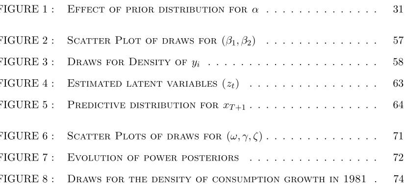
Figure 1Effect of prior distribution for α
(a) # of unique clusters (DPM) (b) # of unique clusters (ET-DPM)
(c) Initial prior (α) (d) Implied prior (α)
Note: The grey line corresponds to a low mean prior for αand the black line corresponds to a high mean αprior. All figures are histograms based on 10,000 draws from the prior distribution described in the main text.
Figure 1 illustrates the relationship between α and the number of unique clusters implied
by the prior choice for α. I generate 10,000 prior draws from the MR-DPM prior (using
Algorithm 1) and the DPM prior (without moment restrictions) with high and low means
for the initial prior distribution for α. For the MR-DPM prior, I use instrumental variable
regression moment restrictions that will be revisited in the upcoming simulation chapter.
Prior specifications for other parts of the prior are the same as those used later. I focus on
the effect of the initial prior distribution for α. Panel (a) shows a histogram of the number
of clusters for the DPM prior based on two prior specifications for α with low (grey) and
This is also true for the DPM prior, as can be seen in Panel (b). However, the MR-DPM prior does not put prior probability on small numbers of clusters owning to the convex
hull condition.5 This effect also can be seen from the implied prior for α (low mean prior).
Compared to the initial prior distribution, the implied prior tends to put less probability
on small α.
2.3.3 Prior specification with a normal kernel function: Beyond the i.i.d.
case
Since the time-series MR-DPM model shares the unknown parameters with the standard
i.i.d.MR-DPM model, the prior distributions imposed on the unknown parameters are very
similar. For models with latent variables, there are two additional unknown parameters
vis-`a-vis i.i.d. MR-DPM models. The first additional unknown is a vector of latent variables, z0:T whose transition probability is known up to finite dimensional parameter βz. I impose
a prior distribution on the initial value for the latent variable, z0. The second additional
unknown isβz. As this parameter is finite dimensional, one can impose a parametric proper
prior distribution.
For example, if the latent variable zt is assumed to follow the univariate AR(1) with a
Gaussian shock,
zt=cz+ρzzt−1+ez,t, ez,t∼N(0,1),
one needs to impose prior distributions on cz,ρz, andz0. In the subsequent application, I
will impose
cz ∼N(mcz, Vcz), ρz∼N(mρz, Vρz), z0 ∼N
0, 1
1−ρ2 z
.
Chapter 3
Posterior analysis
The goal of this chapter is to develop a series of methods that allow for the analysis of
posterior distributions derived from the J-truncated MR-DPM model presented in chapter
2.1 with priors as specified in chapter 2.3 and the joint posterior distribution of model
parameters defined as
p(θ, β, V, α, ψ|X)∝p(X|θ, β, V)p(θ|ψ)p(V|α)p(β)I(~0∈H(θ, β))p(ψ)p(α), (3.1)
wherep(X|θ, β, V) is the likelihood function given by equation 2.13 for an i.i.d.model and
equation 2.19 for a time-dependent model.1 I denote X as x
1:N or x1:T depending on the
context. For models with latent variables, I splice βZ and z0:T into the vector of unknown
parameters and consider the posterior distribution for the augmented unknown parameter
vector, p(θ, β, V, α, ψ, βz, z0:T|X) based on the likelihood function given in equation 2.21.
More specifically, I study three simulation-based posterior samplers that generate samples
from the posterior distribution which can be used to approximate the posterior moments of a
in the moment condition,
E[h(β)|X] =
Z
h(β)π(β)dβ,
where I denote π(β) as the marginal posterior distribution of β and h(∙) is some function that will be clarified later. For example, ifh(β) =β, the above quantity is simply a posterior
mean of β. Since the model specifies the underlying data generating process explicitly, it is
also possible to approximate posterior moments of functionals of the underlying distribution
such as the posterior mean for the data density f(x0; GeJ) at the pointx0,
E[f(x0; GeJ)|X] = Z XJ
j=1 e
qj(θ, β, V)k(x0; θj)π(θ, β, V)d(θ, β, V)
whereπ(θ, β, V) is the marginal posterior distribution.
Another important quantity of interest is the marginal likelihood,
p(X) =
Z
p(X|ϕ)p(ϕ)dϕ,
where ϕ = (θ, β, V, α, ψ). The marginal likelihood plays an important role in Bayesian
analysis as it can be used to compute the posterior model probability. This, in turn, can
be used to obtain the Bayes factor between two competing models for model selection.
In addition, the posterior model probability can be used to compute weights for model
averaging.
The rest of the chapter is organized as follows. First, I introduce the basic posterior sampler
based on the Metropolis-within-Gibbs algorithm and provide conditions under which this
sampler converges to the true posterior distribution as the number of simulations increases.
Second, I introduce a modified version of the basic sampler using a data-augmentation
method that improves the mixing properties of the posterior sampler, as well as computation
3.1
Basic sampler and its convergence
The posterior sampler that I introduce in this subchapter will be called the basic sampler.
The sampler is based on the Metropolis-within-Gibbs algorithm, which cycles over each
parameter of the blockϕ= (θ, β, V, α, ψ) in order; a sequence of draws from this algorithm
defines a Markov chain with a transition kernel KB(ϕ∗|ϕ0) on the product set D=S(θ,β)×
(0,1)J × R+ ×supp(ψ), where supp(ψ) is the domain of the prior distribution for the
hyperparameters.
Algorithm 2. Basic sampler for the J-truncated MR-DPM model. Enter the
following steps with (θ0, β0, V0, α0, ψ0)∈D and i= 1:
1. Draw θj∗ fromp(θj|θ1:∗j−1, θj0:J, β0, V0, α0, ψ0, X), for j= 1, ..., J.
2. Draw β∗ from p(β|θ∗, β0, V0, α0, ψ0, X)
3. Draw Vj∗ fromp(Vj|θ∗, β∗, V1:∗j−1, Vj0:J, α0, ψ0, X), for j= 1, ..., J.
4. Draw α∗ from p(α|θ∗, β∗, V∗, α0, ψ0, X)
5. Draw ψ∗ fromp(ψ|θ∗, β∗, V∗, α∗, ψ0, X)
6. Store (θi, Vi, βi, αi, ψi) = (θ∗, V∗, β∗, α∗, ψ∗). Stop if i=Ns; otherwise, set
(θ0, β0, V0, α0, ψ0) = (θ∗, β∗, V∗, α∗, ψ∗)
and go to step 1 with i=i+ 1.
Under the multivariate normal kernel and prior specification described in the previous chap-ter, a closed-form conditional posterior distribution for α and ψ is possible. However, the
conditional posterior distributions for θ,β, and V are not well-known parametric
algorithm to draw θ, β, and V from the conditional posteriors. The step for parameters
in the mixture kernel function θ depends on the choice of the kernel function and can be
further decomposed into smaller blocks. In the case of the multivariate normal kernel
func-tion, I decompose θj into its mean and variance-covariance matrix, θj = (μj,Σj) for each
j= 1, ..., J and update μj and Σj separately. The variances of each RWMH proposal
den-sities are adaptively chosen following Atchad´e and Rosenthal (2005) so that the resulting
acceptance rates are about 30%. A detailed derivation of the posterior sampler is presented
in the appendix.
When there are latent variables in the model, I add RWMH steps for βz and z0:T to the
previous algorithm. The conditional posterior distributions to update these parameters are
model-specific and can be different depending on the relationship between the observed
data and the latent variables. The following algorithm is based on the example described
in chapter 2.2, where zt follows an AR(1) process and the distribution of xt depends only
on zt.
Algorithm 3. Basic sampler for the J-truncated MR-DPM model with latent
variables. Enter the following steps with (θ0, β0, V0, α0, ψ0, βz0, z0:0T) and i= 1:
1. Draw (θ∗, β∗, V∗, α∗, ψ∗) based on steps 1 – 5 of Algorithm 2 with the likelihood
func-tion defined in equafunc-tion 2.21 and prior distribufunc-tions described in chapter 2.3.
2. Draw βz∗ from p(βz|θ∗, β∗, V∗, α∗, ψ∗, βz0, z0:0T, X).
3. Draw z0∗ using the conditional posterior p(z10|z0, βz∗)p(z0|βz∗).
4. Draw zt∗ using the following conditional posterior:
p(zt|zt∗−1, βz∗)p(xt|zt, θ∗, V∗, β∗)p(z0t+1|zt, βz∗), for 1≤t≤T−1.