R E S E A R C H A R T I C L E
Open Access
Developing a framework for growth
modelling in a managed southern black
beech forest
Elias Ganivet
1*, Elena Moltchanova
2and Mark Bloomberg
1Abstract
Background:A model of individual tree growth using simple predictors in a managed black beech (Fuscospora solandri(Hook.f.) Heenan & Smissen) forest could provide a useful tool for predicting future stand characteristics. Methods:Data from permanent sample plots were used to develop a framework for modelling individual tree growth in Woodside forest, a managed black beech forest in north Canterbury (New Zealand). We tested three mixed-effect models to identify effects of sites, treatment (thinnings), individual tree size and competition on tree growth rates.
Results:A power function amended with variables specifying stand basal area and thinning treatment was best suited for black beech, explaining about 55% of the variation in growth rates. Treatment history (thinnings), as well as the individual tree size and the stand basal area, strongly affected tree diameter growth. Only 3% of the variation in diameter growth rates was explained by plot-specific effect which was less than observed in earlier studies. Conclusions:All predictor variables (management history, individual tree diameter and stand basal area) are quite simple to measure in the field and could be easily used to predict diameter increments in managed or unmanaged forests. A limitation of our study was that available growth data in Woodside were from small plots, focused on a small number of trees and a narrow range of diameters. However, our results are a good starting point, providing a promising framework for further modelling of tree growth in Woodside forest from new permanent plot data.
Keywords:Mixed-effect models, Woodside forest, Black beech forest, Forest management, New Zealand
Background
New Zealand’s native forests cover in total over 6.6 million hectares, with beech forests (dominated by Fuscospora and Lophozonia species) being the most widespread (Wiser et al. 2011). The beech species con-stitute the largest native timber resource remaining in New Zealand, accounting for 88% of the annual allow-able harvest from all indigenous forests under Forests Act requirements (Richardson et al. 2011). Harvesting these forests while maintaining or enhancing their non-extractive benefits has been a controversial issue over the last few decades (Benecke 1996; Mason 2000). As a consequence, native forest harvest is highly regulated,
with only a small part of New Zealand’s privately owned forest covered by sustainable management plans approved by the Ministry for Primary Industries (Donnelly 2011).
Understanding the factors influencing tree growth is a critical task in forest ecology and management. Long-term vegetation monitoring through permanent plots is widely used to provide an insight into regeneration be-haviour and vegetation dynamics as well as growth and mortality patterns (Bakker et al. 1996). Data from per-manent plots allow study of the effects of many factors on tree growth through mathematical models, providing useful tools for forest management (Alder 1995; Boot and Gullison 1995; Alder 2002). In this study, we use data from permanent sample plots in a mono-specific black beech forest (Fuscospora solandri (Hook.f.) Heenan & Smissen) to develop predictive models of * Correspondence:[email protected]
1Department of Land Management and Systems, Faculty of Agribusiness and Commerce, Lincoln University, Lincoln 7640, New Zealand
Full list of author information is available at the end of the article
diameter growth, excluding tree height and mortality rates in our analysis.
Tree growth varying with ontogeny is a well-recognised concept in ecology (Clark and Clark 1999; Poorter et al. 2005; Herault et al. 2011). It has been sug-gested that tree growth rate could be mechanistically re-lated to size by an invariant power law (Enquist et al. 1999; Enquist 2002). This approach has been already used in New Zealand for describing the relationship between the size of an individual and its growth rate (Richardson et al. 2009, 2011). However, the assumption that tree growth rate is only dependent on tree size is suspect, because it is obvious that other factors such as competition and site productivity also influence tree growth (Coomes 2006; Reich et al. 2006; Muller-Landau et al. 2006).
Moreover, while power-law-based approaches only allow a monotonic increase or decrease of growth (Coomes and Allen 2007; Richardson et al. 2009, 2011), some studies argue for hump-shaped growth trajectories, with species attaining their maximum growth rate at intermediate size (Davies 2001; Herault et al. 2011; Easdale et al. 2012). Describing the rela-tionship between the size of an individual and its growth rate has been a debate over the last decade, with authors proposing either one approach or the other (Enquist et al. 1999; Coomes and Allen 2007, 2009; Enquist et al. 2009; Richardson et al. 2011; Herault et al. 2011).
In this study, we aimed to identify which approach is best suited for modelling the relationship between tree size and tree growth rate of a managed black beech for-est in New Zealand. We used multilevel (i.e. mixed) modelling approaches to account for the nested struc-ture of our dataset (trees grouped within plots). Follow-ing earlier studies (Coomes and Allen 2007; Easdale et al. 2012), the basal area of the larger neighbours (BL)
and all neighbours (BT) was also added to the model to
describe competitive effects of such neighbours on growth. Because taller neighbours intercept light first, the basal area of larger neighbouring trees has been often used as a proxy of competition for light. By similar reasoning, basal areas of all neighbouring trees can be used as proxy of above- and below-ground competition (competition for nutrients/water and competition for light).
In New Zealand, some studies have already modelled growth of beeches (Harcombe et al. 1997; Richardson et al. 2011; Coomes et al. 2012; Easdale et al. 2012) and other native species (Kunstler et al. 2009). However, they only focused on unmanaged stands, which does not give information about silvicultural management impacts on growth processes. This study aims to develop a frame-work for modelling individual tree growth using simple
predictors in a managed black beech forest where har-vesting and thinning take place. Such a model could pro-vide a useful tool to predict future stand structure from simple field measurements of tree diameter and stocking.
Methods Study site
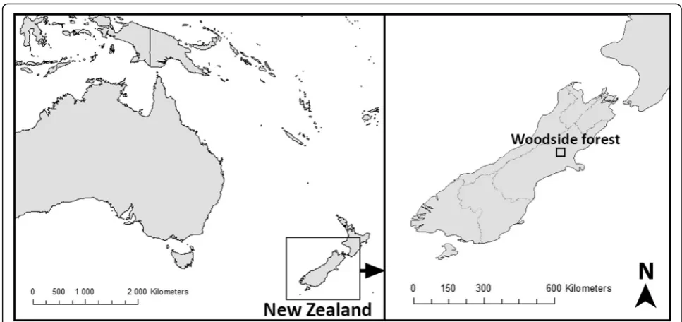
The study was conducted in Woodside, a 121-ha black beech forest privately owned and located in Canterbury in the South Island of New Zealand (Fig. 1). This forest is a part of one of the larger remnants of the formerly extensive Canterbury foothill forests dominated by black beech (Allen et al. 2000). It is a second-growth forest following earlier logging and fire (1860–1910), with management aimed at being an example of sustainable forest management (Allen et al. 2012).
Woodside forest is located at the foothills of the Southern Alps, at an elevation ranging from 400 to 550 m. The climate is windy, with annual precipitation about 1300 mm year−1and common snowfall in winter. The ecology of the forest is affected by location. Infre-quent, heavy, wet snowfalls and recurrent gale-force north-west winds can damage the canopy and potentially expose trees to pests and diseases. The majority of the property is covered by black beech while a smaller area (29 ha) is planted with exotic species (principally Pinus radiata D.Don) for wood production. Of the 84 ha of black beech forest, 70 ha are managed with timber har-vesting as an objective. The remaining 14 ha are man-aged as a reserve with no timber harvesting. The management regime involved aims to work with the eco-logical processes that naturally determine the forest structure.
Data collection
We analysed data from eight rectangular permanent plots of different sizes established by the owner be-tween 2002 and 2006 across the 70 ha of managed black beech forest (Table 1). No plots were established in the unmanaged reserve areas. All black beech trees inside the permanent plots with a diameter at breast height (DBH) ≥1 cm had been identified by the owner. The DBH of each tree had been measured and re-corded, and trees had been tagged with a permanent number using a metal tag and wire. All the plots had been re-measured by the owner at least once, providing DBH increment data for a small sample of trees in Woodside. Six plots had been thinned and pruned, while two plots had received no silvicultural treatments (Table 1).
years between measurements. Some values were excluded from the analysis following Richardson et al. (2011) to account for possible errors in the dataset (dur-ing measurements, record(dur-ing or data entry). We as-sumed negative growth >0.2 cm year−1 and positive growth >1.5 cm year−1to be erroneous, and these values were removed from the dataset prior to analysis. Finally, stand structure parameters of the plots were used as proxy of competition (Coomes and Allen 2007). A proxy of competition for light was defined as the sum of basal areas of trees that had diameters larger than the target tree within the plots. A proxy of above- and below-ground competition (roots, light, etc.) was defined as the basal area of all trees within the plots, excluding the tar-get stem. Finally, because our data were obtained from eight plots with two different management treatments, thinned (plots 1, 2, 3, 4, 6 and 7) and unthinned (plots 5 and 8), we also included a binary factor in the model to assess the impact of thinning on tree growth rates.
Growth models
We tested three candidate growth models using mixed-effect modelling approaches. Mixed-mixed-effect models form a class of model that incorporates multilevel hierarchies in data and can account for the nested structure of our dataset. Allen et al. (2000) found that plot-level variables explained about 40% of the variation in growth rates in Woodside. For that reason, we included the plot-specific effect as a random intercept in all our models.
Power function only (Enquist model)
We first focused on the Enquist growth model (Enquist et al. 1999), also used by Richardson et al. (2011), which models the relationship between tree size and tree growth rate with the following power function:
AGRi¼λ1DBHαi ðM1Þ
which can be linearised as:
Table 1Size, structure and silvicultural history of the eight permanent plots used for the analysis
Plot Treatment Harvesting history Basal area (m2ha−1) Stand density (stems ha−1) Mean DBH (cm) Plot size (m)
Plot 1 T/P – 34.8 1594 15.8 8 × 40
Plot 2 T/P – 16.0 1758 8.6 8 × 32
Plot 3 T/P 1.18 m3removed from dead trees in 2002 25.9 875 17.2 8 × 30
Plot 4 T/P Harvested in 1987 7.9 1344 8.3 8 × 40
Plot 5 – – 40.6 844 22.3 8 × 40
Plot 6 T/P 1.19 m3removed from dead trees in 2005 14.9 2250 8.9 8 × 20
Plot 7 T/P Harvested in 1992 8.6 2750 6.1 8 × 20
Plot 8 – – 51.5 2500 15.4 8 × 20
Tthinned,Ppruned
logAGRi¼ logλ1þαlogDBHiþεi
withεieN 0; σ2 εi
ðM1bÞ
with AGRithe annual growth rate (cm year−1) of the in-dividual tree i; λ1 and α the fitted-model parameters;
DBHi the diameter at breast height (cm) of the individ-ual treeiandεithe fitted-model residuals.
We then added the binary factor for treatment (thin-ning) to the model and accounted for possible plot-related variability by specifying the plots as random effects:
logAGRi¼ logλ1þαlogDBHiþβTiþϕplotiþεi
withϕplot
i eN 0; σ 2 ϕploti
andεieN 0; σ2εi
ðM1cÞ
with AGRithe annual growth rate (cm year−1) of the in-dividual treei; λ1, α and βthe fitted-model parameters;
DBHithe diameter at breast height (cm) of the individ-ual tree i;Tithe treatment effect; ϕploti the plot-specific
effect andεithe fitted-model residuals. Here,Ti= 1 if the observation i comes from an unthinned plot andTi= 0 otherwise.
Power function with competition functions (Coomes model) The method proposed by Coomes and Allen (2007) adjusts and tests for the possible effect of competition by amending M1 with competition functions (e.g. Canham et al. 2004; Uriarte et al. 2004) as follows:
AGRi¼ λ1
DBHαi
1þλ1λ2eλ3BL
1þλ4BT
ð Þ ðM2Þ
which can again be partially linearised, with adjustments for plot effects and for the possible treatment effect as follows:
logAGRi¼ logλ1þαlogDBHi−log 1þλλ1
2e
λ3BL
−log 1ð þλ4BTÞ þβTiþϕplotiþεi:
withϕplotieN 0; σ
2
ϕploti
andεieN 0;σ2εi
ðM2bÞ
with AGRi the annual growth rate (cm year−1) of the individual tree i; λ1, λ2, λ3,λ4, α andβthe fitted-model
parameters; DBHi the diameter at breast height (cm) of the individual treei;BLthe basal area (m2ha−1) of taller neighbours only (proxy of competition for light); BTthe basal area (m2 ha−1) of all neighbours (proxy of above-and below-ground competition); Ti the treatment effect;
ϕploti the plot-specific effect andεi the fitted-model re-siduals. Again,Ti= 1 if the observationi comes from an unthinned plot andTi= 0 otherwise.
Quadratic model of ontogenetic growth trajectories
Finally, we introduced a mathematical model of onto-genetic growth trajectories that has been already de-scribed as the tree-size effect (King et al. 2006; Herault et al. 2010). We used the ratio between the individual DBH and the 95th percentile of the DBH values in the black beech population (DBH95 = 50.46 cm), estimated using inventory data (Ganivet and Bloomberg, unpubl.). Both the ratio and the squared ratio were included to obtain a flexible mathematical form allowing a mono-tonic increase, a monomono-tonic decrease or a humped growth trajectory. In order to remain consistent with M1 and M2 and due to strong heteroscedasticity in our data, the logarithm of growth was modelled instead of growth itself.
The quadratic mathematical model of ontogenetic growth trajectories was specified as follows:
logAGRi¼λ1þλ2
DBHi
DBH95þλ3
DBHi
DBH95
2
þλ4BTþλ5BLþβTiþϕplotiþεi
withϕplotieN 0; σ2ϕploti
andεieN 0;σ2εi
ðM3Þ
with AGRithe annual growth rate (cm year−1) of the in-dividual tree i; λ1, λ2, λ3, λ4, λ5 and β the fitted-model
parameters; BL the basal area (m
2
ha−1) of taller neigh-bours only;BTthe basal area (m2ha−1) of all neighbours; DBHi the diameter at breast height (cm) of the indi-vidual tree i; DBH95 the 95th percentile of the DBH values of black beech; Ti the treatment effect; ϕploti
the plot-specific effect and εi the fitted-model resid-uals. Again,Ti= 1 if the observation i comes from an unthinned plot and Ti= 0 otherwise.
Since the three models (M1c, M2b and M3) had the same response variable, logAGRi, they were all compared
using the Akaike Information Criterion (AIC). Moreover, while the models M1c and M3 were linear in parame-ters, the competition model M2b was not. In order to be consistent, all the three models were fitted using the non-linear mixed-effect model function“nlme” from the “nlme” package in R software v.3.2.2 (R Core Team 2015). Finally, out of 305, only 6 observations had AGR values slightly below 0. In order to allow their log to be calculated, these values were all set to 0.01.
Results
mean AGR for these plots was 0.2 cm year−1while the thinned plots exhibited a mean AGR of 0.6 cm year−1. Growth rates varied also widely among individual trees of the same size (Fig. 3).
The AIC for each of the models M1c, M2b and M3 was 630.80, 627.64 and 629.08 respectively. The quad-ratic model of ontogenetic growth trajectories M3 outperformed the power function model M1c but not the power function with competition function model M2b. We then simplified models M2b and M3 using the AIC in a backward selection to choose the most
parsimonious models and avoid over-parameterisation (Legendre and Legendre 1998). The most parsimonious version of the competition model M2b was:
logAGRi¼ logλ1þαlogDBHi−log 1ð þλ4BTÞ
þβTiþϕplotiþεi:
ðM2cÞ
with AGRithe annual growth rate (cm year−1) of the in-dividual tree i; λ1, λ4,α and βthe fitted-model
parame-ters; DBHi the diameter at breast height (cm) of the individual tree i; BTthe basal area (m2ha−1) of all trees around the target stem (within the entire plot); Ti the treatment effect; ϕplot
i the plot-specific effect and εithe
fitted-model residuals.
This final model M2c resulted in AIC = 626.71. Re-moving the term BT would result in M1c which would
decrease the model fit as evaluated by AIC. The most parsimonious version of the quadratic model M3 was:
logAGRi¼λ1þλ2
DBHi
DBH95þλ3
DBHi
DBH95
2
þλ4BTþβTiþϕplotiþεi: ðM3bÞ
with AGRi the annual growth rate (cm year−1) of the individual tree i; λ1, λ2, λ3, λ4 and β the fitted-model
parameters; BT the basal area (m2 ha−1) of all neigh-bours; DBHithe diameter at breast height (cm) of the in-dividual tree i; DBH95 the 95th percentile of the DBH values of black beech; Ti the treatment effect; ϕploti the
plot-specific effect andεithe fitted-model residuals.
This final model M3b resulted in AIC = 627.76, which still outperformed the power model M1c but not the competition model M2c. Comparing the residuals for Fig. 2Diameter annual growth rates across the plots in Woodside.
Theboxesrepresent 25th and 75th percentiles with the median represented byhorizontal bars. Thenumberin eachboxcorresponds to the number of observations.Linesare either extreme values or 1.5 times the interquartile range, andopen dots are outliers. Mean overall AGR = 0.5 cm year−1. Mean AGR in thinned plots =
0.6 cm year−1. Mean AGR in unthinned plots = 0.2 cm year−1
the three models (not shown in the results), the unthinned stands had more variance than the thinned ones. To see whether the growth dynamics were qualita-tively different in the two types of stands, we tested the above models for the interaction effect between treat-ment and DBH. We also tested for plot-specific effects of treatment or DBH, i.e. random slopes. However, none of those features improved any of the three models. The estimated parameters of the final three models are shown in Table 2.
To assess the relative explanatory value of the fixed effects and random intercepts, we evaluated the total variance of the observed response, logAGR, the variance of the random slopes and the residual variance (Table 2). In all three models, about 45% of the variance remained unexplained. In both the competition model M2c and the quadratic model M3b, 51% of the variance was ex-plained by the fixed effects only, against 45% in M1c. The remaining variance explained by the random slopes was only 3% in M2c, 4% in M3b and 9% in M1c.
Trees ranged from 1- to 40-cm DBH in the current dataset, which resulted in the modelled growth rate of black beech exhibiting a dependency on tree size, with growth rates increasing monotonically when diameters increased in the three models (Fig. 3). However, in the quadratic model M3b, the presence of a negative value for the quadratic parameter λ3 allowed for a
hump-shaped response of tree growth to tree diameter. As a mathematical consequence of the low value of λ3, the
AGR only reached a peak at around 140-cm DBH and then decreased at larger diameters. This was not shown in Fig. 2 as our dataset ranged only up to 40-cm DBH.
The observed influence of treatment was substantial in all three models tested, with reduced AGR in unthinned plots (Fig. 3). Growth trajectories were slightly different
among models, with AGR increasing logarithmically with models M1 and M2 while exponentially (from 0- to 40-cm DBH) with model M3. Also, the rate of increase in AGR was greater for model M1 compared with model M2.
Discussion
Large variability in growth rates was observed in this study (Fig. 3). Consistent with the results of Allen et al. (2000), AGR varied widely among the plots (Fig. 2) prov-ing the necessity of includprov-ing the plot effect in our mod-elling approach. Also, as observed by Allen et al. (2000), trees in Woodside exhibited relatively high mean AGR (0.5 cm year−1) compared with what has been found elsewhere, not only for black beech but also the closely related species mountain beech (Fuscospora cliffortioides (Hook.f.) Heenan & Smissen) (see Coomes and Allen 2007; Richardson et al. 2011). This could be partly linked to environmental differences (i.e. elevation, climate, soil, etc.). While the Woodside plots were all located at around 500 m in elevation, the other studies usually in-volved black/mountain beech forests at higher elevations.
However, the high overall mean AGR was due mainly to the thinned plots (mean AGR of 0.6 cm year−1). The mean AGR in unthinned plots 5 and 8 was only 0.2 cm year−1which was consistent with what has been found elsewhere for black and mountain beeches. Thus, it seems the main driver of these differences in AGR would be the silvicultural management occurring at Woodside (i.e. thinning), which aims to improve individ-ual tree growth. The positive impact of thinning on tree growth rates was further confirmed by the three model-ling approaches tested. They all presented a significant effect of treatment, with clearly lower growth rates in unthinned stands (Fig. 3). For all models, there was no
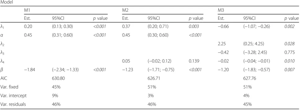
Table 2Summary of the estimated parameters, resulting AIC and relative variance of the response logAGR explained by the fixed effects, random intercepts and residuals (unexplained) for the three tested models
Model
M1 M2 M3
Est. 95%CI pvalue Est. 95%CI pvalue Est. 95%CI pvalue
λ1 0.20 (0.13; 0.30) <0.001 0.37 (0.20; 0.71) 0.003 −0.66 (−1.07;−0.26) 0.002 α 0.45 (0.31; 0.60) <0.001 0.45 (0.30; 0.60) <0.001
λ2 2.25 (0.25; 4.25) 0.028
λ3 −0.42 (−3.28; 2.45) 0.775
λ4 0.05 (−0.02; 0.12) 0.139 −0.02 (−0.04;−0.01) 0.010
β −1.84 (−2.34;−1.33) <0.001 −1.23 (−1.71;−0.75) <0.001 −1.20 (−1.83;−0.57) 0.007
AIC 630.80 626.71 627.76
Var. fixed 45% 51% 51%
Var. intercept 9% 3% 4%
Var. residuals 46% 46% 45%
evidence that the effect of individual size on AGR was different in thinned vs. unthinned stands.
The best model was M2 in terms of AIC, although the differences among the three models were relatively small. Model M2 included a competition function (basal areas of all neighbours), which increased the variance explained by the fixed effects (51%). This result suggests that, as expected, black beech growth depends also on resource availability as an effect of above- and below-ground competition. It was further consistent with re-sults from Coomes and Allen (2007) and other studies that already outlined effects of root competition (Platt et al. 2004), especially for nitrogen (Davis et al., 2004), on mountain beech. The power function model M1 was outperformed by both M2 and M3, supporting other studies that have shown that simplistic power-law func-tions are not generally the best descriptors of tree growth (Vanclay 1995; Coomes and Allen 2007, 2009; Enquist et al. 2009).
In terms of growth trajectories, our data were best de-scribed by M2 which exhibited a monotonic increase of the AGR with increasing diameters (Fig. 3). This result contrasted with other studies in New Zealand (Easdale et al. 2012) and elsewhere (Kohyama et al. 2003; Uriarte et al. 2004; Coates et al. 2009) that reported a hump-shaped response of growth to tree diameter. However, a clear limit of our dataset was the small diameter range (DBH≤40 cm) compared with results from other studies in Woodside that used inventory data of larger diameter trees (Allen et al. 2000; Ganivet and Bloomberg, unpubl.). This lack of growth data for larger trees in the current study may explain the late humped growth re-sponse in M3 and why the quadratic model did not per-form as well as M2. Maximal growth rates would be expected to be reached at intermediate sizes (around 30–50-cm DBH), while the AGR peaked at around 140-cm DBH in M3 before decreasing. New data with larger tree diameters would be required to re-estimate the pa-rameters and compare M3 with M2. In any case, the monotonic growth trajectory found in this study was consistent with other studies on black and mountain beech (Coomes and Allen 2007; Richardson et al. 2011). Different factors could be relevant to explain this in-crease in growth with tree ontogeny.
At young stages, lower growth rates could be caused by: (1) black beech trees initially putting energy into height growth rather than diameter growth (Wardle, personal communication); and/or (2) a lack of available resources such as light (Chazdon et al. 1996; Whitmore 1996). Our proxy of competition for light (BL) did not
improve the tested models when used as an explanatory variable. However, light is widely accepted to be one of the main environmental limiting factors for tree growth (Pacala et al. 1996; Smith et al. 1997; Herwitz et al. 2000;
Canham et al. 2004; Uriarte et al. 2004; Wyckoff and Clark 2005), especially for light-demanding species such as black beech (Wardle et al. 1984). Our results suggest that using basal areas of taller trees as proxy of light competition is either not relevant or it needs to be mea-sured at a smaller scale than the whole plot (see Coomes and Allen 2007). Light is more variable in the under-storey than in the sub-canopy and canopy, so small-size trees are necessarily more dependent on variation in light availability than large trees (Wright et al. 2010). For larger diameter trees, increase in growth rates could be a consequence of trees reaching canopy status and spread-ing their crown, which further enhances light capture and growth (Poorter et al. 2006).
The aim of our study was to develop a simple frame-work that could be used for predictions, rather than explaining all the possible variation in growth rate. A model was successfully developed that explained more than 50% of the variation in growth rates using only few predictors easily measurable in the field (management history, individual tree diameter and stand basal area). However, a substantial fraction of individual variation in growth remained unexplained in all three modelling ap-proaches used. This means other factors not investigated here might contribute to influence the growth of black beech in this managed forest. Depending on the model used, the plot-specific effect only explained 3–9% of the variation in growth rates, which was much less than the 40% found by Allen et al. (2000). However, their analysis did not look for effect of management on tree growth, and it is likely that our variable for treatment included a substantial fraction of the unaccounted plot-specific effect.
In February 2016, a further twelve 0.07-ha permanent plots were established across Woodside forest (Ganivet and Bloomberg, unpubl.). Further growth data from these permanent plots will provide additional data for building a more accurate model for the management of trees in this forest. Moreover, the spatial organisation of trees in the plots were measured, and these data could be used to investigate effects of competition for light at a smaller scale. A final recommendation would be to in-clude mortality rates in the model to improve yield predictions.
Conclusions
the variation in growth rates remained explained by the plot-specific effect. These predictors are quite simple to measure in the field and could be easily used to predict diameter increments in managed or unmanaged forests. The growth data used focused on a small number of trees, a narrow range of diameters (up to 40 cm only) within a small geographic area, which limited the applic-ability of the model even though it performed well. Moreover, contrary to our expectations, the method did not produce reliable results when a basal area parameter was used as a proxy of competition for light. However, the results of the current study provide a good starting point for growth modelling of a southern black beech forest and provide a promising framework for further modelling.
Ethics approval and consent to participate Not applicable
Abbreviations
AGR:Annual growth rate; DBH: Diameter at breast height
Acknowledgements
We thank John and Rosalie Wardle for access to their unique forest. For assistance and advice in the field, we would like to thank Marcel Van Leeuwen (MalvernGIS Ltd) and Michael Pay, student at the School of Forestry, University of Canterbury. The first author acknowledges funding support by theRégion Franche-Comté(France) as part of theStage monde internship programme. Finally, we record our appreciation to John Wardle, Euan Mason and Rob Allen for useful comments on this paper.
Funding
The first author acknowledges funding support by theRégion Franche-Comté (France) as part of theStage mondeinternship programme.
Availability of data and materials
Permanent sample plot data were provided by the landowners (John and Rosalie Wardle). However, they have not consented to making the original measurement data available as an appendix to the report, and this must be obtained by request from the landowners.
Authors’contributions
EG handled the project design, analysis and interpretation of the data and wrote substantial sections of the paper. EM handled the analysis and interpretation of the data. MB supervised the study, including the project design and coordination and assistance with the interpretation of the results and writing the paper. All authors read and approved the final manuscript.
Authors’information
Elias Ganivet: Research and Teaching Assistant in Forestry, Department of Land Management and Systems, Faculty of Agribusiness and Commerce, Lincoln University, Lincoln 7640, New Zealand.
Elena Moltchanova: School of Mathematics and Statistics, University of Canterbury, Christchurch, New Zealand.
Mark Bloomberg: Senior Lecturer in Forestry Management, Department of Land Management and Systems, Faculty of Agribusiness and Commerce, Lincoln University, Lincoln 7640, New Zealand.
Competing interests
The authors declare that they have no competing interests.
Consent for publication
Permanent sample plot data were provided by the landowners (John and Rosalie Wardle), and the analysis and results in this paper are published with their consent.
Publisher’s Note
Springer Nature remains neutral with regard to jurisdictional claims in published maps and institutional affiliations.
Author details
1Department of Land Management and Systems, Faculty of Agribusiness and Commerce, Lincoln University, Lincoln 7640, New Zealand.2School of Mathematics and Statistics, University of Canterbury, Christchurch, New Zealand.
Received: 11 August 2016 Accepted: 22 May 2017
References
Alder, D. (1995).Growth modelling for mixed tropical forests. Oxford: Oxford Forestry Institute, University of Oxford.
Alder, D. (2002). Simple diameter class and cohort modelling methods for practical forest management. In ITTO Workshop on Growth and Yield, Kuala Lumpur, 24th-28th June
Allen, R., Wiser, S., Burrows, L., & Brignall-Theyer, M. (2000). Silvicultural research in selected forest types: a black beech forest in Canterbury. InLandcare Research Contract Report: LC0001/01 for the Ministry of Agriculture and Forestry, Wellington.
Allen, R., Hurst, J., Wiser, S., & Easdale, T. (2012). Developing management systems for the production of beech timber.New Zealand Journal of Forestry, 57, 38–44.
Bakker, J., Olff, H., Willems, J., & Zobel, M. (1996). Why do we need permanent plots in the study of long-term vegetation dynamics?Journal of Vegetation Science, 7(2), 147–156.
Benecke, U. (1996). Ecological silviculture: the application of age-old methods. New Zealand Forestry, 41, 27–33.
Boot, R. G., & Gullison, R. (1995). Approaches to developing sustainable extraction systems for tropical forest products.Ecological Applications, 5(4), 896–903. doi:10.2307/2269340.
Canham, C. D., LePage, P. T., & Coates, K. D. (2004). A neighborhood analysis of canopy tree competition: effects of shading versus crowding.Canadian Journal of Forest Research, 34(4), 778–787. doi:10.1139/X03-232. Chazdon, R. L., Pearcy, R. W., Lee, D. W., & Fetcher, N. (1996). Photosynthetic
responses of tropical forest plants to contrasting light environments. In S. S. Mulkey, R. L. Chazdon, & A. P. Smith (Eds.),Tropical Forest Plant Ecophysiology (pp. 5-55). US: Springer.
Clark, D. A., & Clark, D. B. (1999). Assessing the growth of tropical rain forest trees: issues for forest modeling and management.Ecological Applications, 9(3), 981–997. doi:10.2307/2641344.
Coates, K. D., Canham, C. D., & LePage, P. T. (2009). Above-versus below-ground competitive effects and responses of a guild of temperate tree species.Journal of Ecology, 97(1), 118–130. doi:10.1111/j.1365-2745.2008. 01458.x.
Coomes, D. A. (2006). Challenges to the generality of WBE theory.Trends in Ecology & Evolution, 21(11), 593–596. doi:10.1016/j.tree.2006.09.002. Coomes, D. A., & Allen, R. B. (2007). Effects of size, competition and altitude on
tree growth.Journal of Ecology, 95(5), 1084–1097. doi:10.1111/j.1365-2745. 2007.01280.x.
Coomes, D. A., & Allen, R. B. (2009). Testing the metabolic scaling theory of tree growth.Journal of Ecology, 97(6), 1369–1373. doi:10.1111/j.1365-2745.2009. 01571.x.
Coomes, D. A., Holdaway, R. J., Kobe, R. K., Lines, E. R., & Allen, R. B. (2012). A general integrative framework for modelling woody biomass production and carbon sequestration rates in forests.Journal of Ecology, 100(1), 42–64. doi:10.1111/j.1365-2745.2011.01920.x.
Davies, S. J. (2001). Tree mortality and growth in 11 sympatric Macaranga species in Borneo.Ecology, 82(4), 920–932. doi:10.2307/2679892.
Davis, M. R., Allen, R. B., & Clinton, P. W. (2004). The influence of N addition on nutrient content, leaf carbon isotope ratio, and productivity in aNothofagus forest during stand development.Canadian Journal of Forest Research, 34(10), 2037–2048. doi:10.1139/x04-067.
Easdale, T. A., Allen, R. B., Peltzer, D. A., & Hurst, J. M. (2012). Size-dependent growth responses to competition and environment inNothofagus menziesii. Forest Ecology and Management, 270, 223–231. doi:10.1016/j.foreco.2012.01. 009.
Enquist, B. J. (2002). Universal scaling in tree and vascular plant allometry: toward a general quantitative theory linking plant form and function from cells to ecosystems.Tree Physiology, 22(15-6), 1045–1064. doi:10.1093/treephys/22.15-16.1045.
Enquist, B. J., West, G. B., & Brown, J. H. (2009). Extensions and evaluations of a general quantitative theory of forest structure and dynamics.Proceedings of the National Academy of Sciences, 106(17), 7046–7051.
Enquist, B. J., West, G. B., Charnov, E. L., & Brown, J. H. (1999). Allometric scaling of production and life-history variation in vascular plants.Nature, 401(6756), 907–911. doi:10.1038/44819.
Harcombe, P., Allen, R. B., Wardle, J., & Platt, K. (1997). Spatial and temporal patterns in stand structure, biomass, growth, and mortality in a monospecific Nothofagus solandri var. cliffortioides(hook, f.) Poole forest in New Zealand. Journal of Sustainable Forestry, 6(3-4), 313–345. doi:10.1300/J091v06n03_06. Herault, B., Bachelot, B., Poorter, L., Rossi, V., Bongers, F., Chave, J., Paine, C.,
Wagner, F., & Baraloto, C. (2011). Functional traits shape ontogenetic growth trajectories of rain forest tree species.Journal of Ecology, 99(6), 1431–1440. doi:10.1111/j.1365-2745.2011.01883.x.
Herault, B., Ouallet, J., Blanc, L., Wagner, F., & Baraloto, C. (2010). Growth responses of neotropical trees to logging gaps.Journal of Applied Ecology, 47(4), 821–831. doi:10.1111/j.1365-2664.2010.01826.x.
Herwitz, S. R., Slye, R. E., & Turton, S. M. (2000). Long-term survivorship and crown area dynamics of tropical rain forest canopy trees.Ecology, 81(2), 585–597. doi:10.1890/0012-9658(2000)081[0585:LTSACA]2.0.CO;2.
King, D. A., Davies, S. J., & Noor, N. S. M. (2006). Growth and mortality are related to adult tree size in a Malaysian mixed dipterocarp forest.Forest Ecology and Management, 223(1), 152–158. doi:10.1016/j.foreco.2005.10.066.
Kohyama, T., Suzuki, E., Partomihardjo, T., Yamada, T., & Kubo, T. (2003). Tree species differentiation in growth, recruitment and allometry in relation to maximum height in a Bornean mixed dipterocarp forest.Journal of Ecology, 91(5), 797–806. doi:10.1046/j.1365-2745.2003.00810.x.
Kunstler, G., Coomes, D. A., & Canham, C. D. (2009). Size-dependence of growth and mortality influence the shade tolerance of trees in a lowland temperate rain forest.Journal of Ecology, 97(4), 685–695. doi:10.1111/j.1365-2745.2009. 01482.x.
Legendre, P., & Legendre, L. (1998).Numerical ecology(2nd English ed.). Amsterdam: Elsevier Science.
Mason, E. (2000). Evaluation of a model beech forest growing on the west coast of the South Island of New Zealand.New Zealand Journal of Forestry, 44(4), 26–31.
Muller-Landau, H. C., Condit, R. S., Harms, K. E., Marks, C. O., Thomas, S. C., Bunyavejchewin, S., Chuyong, G., Co, L., Davies, S., Foster, R., et al. (2006). Comparing tropical forest tree size distributions with the predictions of metabolic ecology and equilibrium models.Ecology Letters, 9(5), 589–602. doi:10.1111/j.1461-0248.2006.00915.x.
Pacala, S. W., Canham, C. D., Saponara, J., Silander, J. A., Jr., Kobe, R. K., & Ribbens, E. (1996). Forest models defined by field measurements: estimation, error analysis and dynamics.Ecological Monographs, 66(1), 1–43. doi:10.2307/ 2963479.
Platt, K. H., Allen, R. B., Coomes, D. A., & Wiser, S. K. (2004). Mountain beech seedling responses to removal of below-ground competition and fertiliser addition.New Zealand Journal of Ecology, 28(2), 289–293.
Poorter, L., Bongers, F., Sterck, F. J., & Wöll, H. (2005). Beyond the regeneration phase: differentiation of height-light trajectories among tropical tree species. Journal of Ecology, 93(2), 256–267. doi:10.1111/j.1365-2745.2004.00956.x. Poorter, L., Bongers, L., & Bongers, F. (2006). Architecture of 54 moist-forest tree
species: traits, tradeoffs, and functional groups.Ecology, 87(5), 1289–1301. doi:10.1890/0012-9658(2006)87[1289:AOMTST]2.0.CO;2.
R Core Team. (2015).R: a language and environment for statistical computing. Vienna: R Foundation for Statistical Computing.
Reich, P. B., Tjoelker, M. G., Machado, J.-L., & Oleksyn, J. (2006). Universal scaling of respiratory metabolism, size and nitrogen in plants.Nature, 439(7075), 457– 461. doi:10.1038/nature04282.
Richardson, S. J., Hurst, J. M., Easdale, T. A., Wiser, S. K., Griffiths, A. D., & Allen, R. B. (2011). Diameter growth rates of beech (Nothofagus) trees around New Zealand.New Zealand Journal of Forestry, 56(1), 3–11.
Richardson, S. J., Smale, M. C., Hurst, J. M., Fitzgerald, N. B., Peltzer, D. A., Allen, R. B., Bellingham, P. J., & McKelvey, P. J. (2009). Large-tree growth and mortality rates in forests of the central North Island, New Zealand.New Zealand Journal of Ecology, 33(2), 208–215.
Smith, D. M., Larson, B. C., Kelty, M. J., & Ashton, P. M. S. (1997).The practice of silviculture: applied forest ecology. 9th ed. New York: John Wiley and Sons, Inc. Uriarte, M., Canham, C. D., Thompson, J., & Zimmerman, J. K. (2004). A
neighborhood analysis of tree growth and survival in a hurricane-driven tropical forest.Ecological Monographs, 74(4), 591–614. doi:10.1890/03-4031. Vanclay, J. K. (1995). Synthesis: growth models for tropical forests: a synthesis of
models and methods.Forest Science, 41(1), 7–42.
Wardle, J., et al. (1984).The New Zealand beeches: ecology, utilisation and management. Wellington: New Zealand Forest Service.
Whitmore, T. (1996). A review of some aspects of tropical rain forest seedling ecology with suggestions for further enquiry.Man and the Biosphere Series, 17, 3–40.
Wiser, S. K., Hurst, J. M., Wright, E. F., & Allen, R. B. (2011). New Zealand’s forest and shrubland communities: a quantitative classification based on a nationally representative plot network.Applied Vegetation Science, 14(4), 506–523. doi:10.1111/j.1654-109X.2011.01146.x.
Wright, S. J., Kitajima, K., Kraft, N. J., Reich, P. B., Wright, I. J., Bunker, D. E., Condit, R., Dalling, J. W., Davies, S. J., Díaz, S., Engelbrecht, B. M. J., Harms, K. E., Hubbell, S. P., Marks, C. O., Ruiz-Jaen, M. C., Salvador, C. M., & Zanne, A. E. (2010). Functional traits and the growth-mortality trade-off in tropical trees. Ecology, 91(12), 3664–3674. doi:10.1890/09-2335.1.