IJSRSET1841124 | Received : 01 Nov 2018 | Accepted : 12 Nov 2018 | November-December-2018 [ 4 (11) : 89-95]
Themed Section : Engineering and Technology DOI : https://doi.org/10.32628/IJSRSET1841124
89
Adaptive Control Scheme for Coupled Tank Process
M. Vinodhini
Department of Instrumentation and Control Engineering, A.V.C. College of Engineering, Mannampandal, India
ABSTRACT
The objective of this paper is to develop a Direct Model Reference Adaptive Control (DMRAC) algorithm for a MIMO process by extending the MIT rule adopted for a SISO system. The controller thus developed is implemented on Laboratory interacting coupled tank process through simulation. This can be regarded as the relevant process control in petrol and chemical industries. These industries involve controlling the liquid level and the flow rate in the presence of nonlinearity and disturbance which justifies the use of adaptive techniques such as DMRAC control scheme. For this purpose, mathematical models are obtained for each of the input-output combinations using white box approach and the respective controllers are developed. A detailed analysis on the performance of the chosen process with these controllers is carried out. Simulation studies reveal the effectiveness of proposed controller for multivariable process that exhibits nonlinear behaviour.
Keywords : Coupled tank system, MIMO, DMRAC, MIT rule
I. INTRODUCTION
Most of the industrial processes are Two Input Two Output (TITO) systems which have cross coupling between the process inputs and outputs. Comparing with Single Input Single Output (SISO) counterparts, TITO processes are more difficult to control due to the existence of interactions between input and output variables. Many techniques have been suggested in the past for controlling the TITO systems. Decoupling controllers are used to transform TITO plant transfer function model into SISO form. Thus two degrees of freedom PI controller for each of the SISO models can be designed by Root Locus Technique [1].
Chatchaval et al.[2] has implemented a decentralized fuzzy logic controller for TITO coupled tank process. Suparoek et al. [3] has presented a design methodology of auto-adjustable PI controller using
Model Reference Adaptive Control (MRAC)
technique for solving the problem of coupled tank process as fixed controllers are not able to provide efficient control in the presence of disturbance and variation in parameters.
Recently Asan Mohideen et al. [4] has designed a MRAC with a very good steady state and transient performance for a nonlinear process such as the hybrid tank process. Rathikarani et al. [5] proposed an auto tuning of the PI controller using MRAC concept for a nonlinear air flow process. Bharathi et al. [6] have considered continuous time adaptive control to a nonlinear two tank non-interacting SISO system.
International Journal of Scientific Research in Science, Engineering and Technology (www.ijsrset.com)
90
convenient for controller design satisfying the system requirement.
The paper is organized as follows: The laboratory interacting coupled tank process setup chosen for the study is detailed first. Then the methodology used for modeling and the validation of multiloop process is outlined. After a brief introduction about multiloop PI controller, the procedure involved in developing DMRAC is presented. The performance analysis of the proposed controller is reported before providing the conclusion
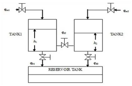
II. PROCESS DESCRIPTION
The schematic diagram of the chosen Interacting coupled tank system is illustrated in Fig. 1.
The mass balance equations of tank1 and tank2 are given in Equations 1 and 2. The rate of change of liquid volume in each tank is equal to the net flow of liquid into the tank. The volumetric inflow rate into the tank1 and tank2 are qin1 and qin2. The volumetric
flow rate from the tank1 and tank2 are q01 and q02.
Flow rate between tank1 and tank2 is q12. The height
of the liquid level is h1 in tank1 and h2 in tank2.
12 1 1 1
1 q q q
dt dh
A in o
(1) 12 2 2 2
2 q q q
dt dh
A in o (2)
The system model can be formulated by ordinary differential equation using Bernoulli’s law as shown in Equations 3 and 4.
) ( 2
2 1 2
1 12 1 1 1 1 1
1 g h h
A a gh A a A q dt
dh in (3)
) ( 2
2 1 2
1 12 2 2 2 2 2
2 gh h
A a gh A a A q dt dh in
(4)
The cross sectional area of tank1 and tank2 are A1=A2=1130.4cm2, restriction areas in the outlet pipes
of tank1 and tank2 are a1=a2= 3.9cm2. Restriction area
of interconnecting pipe is a12=1.27cm2 and g is the
specific gravity. The maximum capacity of two tanks is 25cm. Equations 3 and 4 describe the coupled tank system dynamics. To design the control systems for
this process the equations are linearized by considering small variations in qin1, qin2, h1 and h2 [3].
Fig. 1. Schematic diagram of coupled tank process
The variations are measured with respect to nominal operating conditions. The hand valves are adjusted so that the levels in both the tanks are brought to nominal condition initially. Nominal values of qin1,
qin2 are 26 and 20.75 l/hr and for h1 and h2 are 12.5 and
12.1cm respectively.
The linearized models of the process are given below in Equations 5. Based on this structure, the reference model for the MRAC is to be decided.
Rearranging the equations (3) & (4) and then taking laplace transform on both sides, we get
( ) ( )
1)
( 1 12
1 1
1 q s q s
s R s
h in
( ) ( )
1 )( 2 12
2 2
2 s q s q s
R s
h in
III. MULTILOOP PROCESS
The four models relating the two controlled outputs h1 and h2 with two manipulated inputs qin1 and qin2 are
essential to design the multiloop controllers [5]. The model transfer functions with the flow rates as manipulated inputs and the levels as controlled outputs can be written as follows:
The open loop response of the process for a 10% change in qin1 is plotted in Fig. 2. This causes the level
in tank1 to change from 12.5cm to 20cm. Due to
interaction, level in tank2 reaches the steady state
value 16.5cm from its nominal value. Figure 3 displays the graphs for variation in qin1 and qin2 in
nominal condition.
Fig. 3. Variation of qin1
In the same manner, the open loop responses (as in Fig. 4) are obtained by making 10% change in qin2
maintaining qin1 in nominal condition. Here also the
level in tank1 reaches steady state at 18cm. Figure 5 displays the graphs for variation in qin2 and qin1 in
nominal condition.
Fig. 4. Openloop response for the process (∆qin2)
Fig. 5. Variation of qin2
The Transfer functions are computed and represented in matrix form as follows:
s . s
. s
. s
.
G G
G G G
1 81
633 0 1 106
443
0 111 1
583 0 1 61
737 0
22 21
12
11
A .Validation
Model validation is the most important step of model building and is accomplished by matching simulated output from white box approach (Actual output) with
transfer function model (model output).
Implementation of the model without validation may lead to erroneous and misleading results. So it is essential to verify the model. Figures 6(a) and (b)
shows the time domain validation for the models G21
andG22 respectively.
Fig. 6(a). Time domain validation for the model G21
Fig. 6(b). Time domain validation for the model G22
The block diagram of Multiloop control system of a
coupled tank process employed with Gc1 and Gc2 as PI
controllers for tank1 and tank2 is shown in Fig. 7 [7].
400 600 800 1000 1200 1400
12 14 16 18 20
Sampling instants
L
ev
el
in
c
m
h1 h2
400 600 800 1000 1200 1400 20
25 30 35
Sampling instants
F
lo
w
i
n
L
P
H
qin1 qin2
600 800 1000 1200 1400
12 13 14 15 16 17
Sampling instants
L
ev
el
i
n
c
m
Model Output Actual output
600 800 1000 1200 1400
12 14 16 18
Sampling instants
L
ev
el
i
n
c
m
Model Output Actual Output
International Journal of Scientific Research in Science, Engineering and Technology (www.ijsrset.com)
92
Fig. 7. Multiloop PI control system
Synthesis Method of Tuning
The PI controller parameters are tuned using synthesis method for the two first order processes G11 and G22 obtained from modelling. Kc is proportional gain. Ti is integral time. Ki is integral gain. τc is closed loop time constant of the process.
Controller parameters are determined and tabulated in Table I.
Table I. Controller Parameters for PI Controller
Parameters Controller
Gc1 Gc2
τ k
τ K
c p
p
c 2.357 2.579
T K K
i c
i 0.038 0.032
IV.Direct Model Reference Adaptive Controller
The block diagram of Multiloop DMRAC system is shown in Fig. 8. This system consists of a reference model, parameter adjustment mechanism and controller in each loop in order to control the two controlled outputs. The reference model describes the desired input/output character of the closed loop system. The controller drives the control signal so that the closed loop characteristics from the setpoint
(hspi) to the process output hi (where i=1,2 represents
the control loops) is equal to the dynamics of the
reference model (hm). In this work, the reference
model is selected with the gain 1 and time constant 0.5. Matching the process and reference model dynamics guarantees the convergence of the
modeling error (ei) to zero. The controller drives the
difference (error) between the process response and
desired model output to zero asymptotically at a rate
constrained by the adaptation gain (ע).
The designed controller has a conventional inner loop followed by a adaptive outer loop to adjust the controller parameters for the respective loops based on the modeling error such a way that the coefficients of the model and the closed loop plant are equal [8].
Here the modeling error,
ei=hi-hm (8)
A.MIT Algorithm
The controller parameters (θni) is adjusted with the
constraint given by following loss function,
2
2 1
) i
ni e
J(θ (9)
where n=1,2 represents controller parameter number. In order to minimize the loss function J, the parameters can be changed in the direction of negative gradient of J. The following parameter adjustment mechanism is called MIT algorithm [9].
(9)
(10)
The quantity
ni i
e
is the sensitivity derivative of
the error with respect to controller parameters. The
parameter,
determines the adaptation rate. Basedon the apriori knowledge, the linearized model of the chosen nonlinear process around a specific operating condition is represented as follows:
i i
i i pi
a s
b u h G
(11) where bi , ai are process parameters. Assuming hspi as the setpoint and ui the control signal, the MIT control law can be written as in equation (11).
i i spi i
i θ h h
u 1 2 (12)
By substituting equation 12 in 11, the closed loop transfer function with MRAS is obtained as,
Fig.8. Block diagram of Multiloop DMRAC system
θ e γe θ
J γe dt dθ
ni i i ni i ni
(13)
Based on the equation 13, the transfer function of the model is given by
m m spi m m a s b h h G
(14)
where bm , am are the model parameters. Under the
exact model following condition, the controller parameters are given by equation 14.
i i m i i m i b a a θ b b
θ1 and 2 (15)
By substituting equations 13 and 14 in equation 8, the modeling error is obtained as follows:
spi m m spi i i i i i i h a s b h θ b a s θ b e 2
1 (16)
The sensitivity derivatives are obtained by taking partial derivatives with respect to the controller parameters. i i i i i i i spi i i i i i i h θ b a s b θ e h θ b a s b θ e 2 2 2 1 and (17)
By substituting equations 17 in equation 10, the rate
of change of controller parameters 1 2
dt dθ , dt
dθi i are given
by equations 18.
i m m i i spi m m i i h a s a γe dt dθ h a s a γe dt dθ 2 1 and (18)
By varying adaptation gain (
), tracking speed and the convergence rate of controller parameters are varied.V. Simulation Results
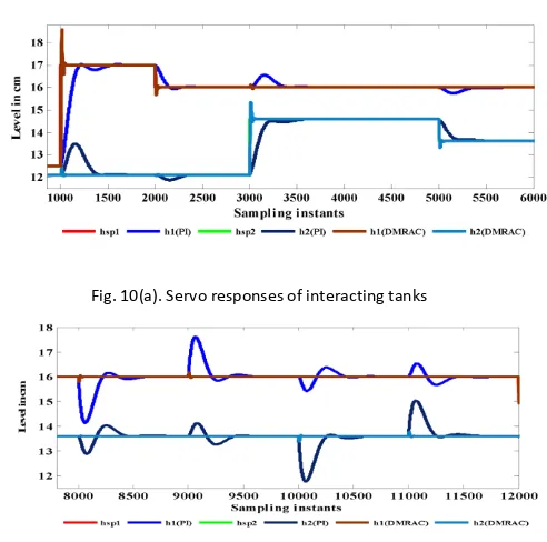
The Fig.9 shows the enlarged servo responses of interacting tanks (∆h1). The adaptation gain used in the controllers is 0.2. Figure 10(a) and (b) shows the servo and regulatory responses of interacting tanks.
Positive change in hsp1 (Servo 1) from 12.5 to 17cm is
given at 1000th sampling instant as shown in Fig.
10(a). Negative change of 1cm in hsp1 (Servo 2) is
applied at 2000th sampling instant. Due to the action
of DMRAC1 in loop1, the level in tank1 tries to track the setpoint. Due to interaction h2 slightly oscillates
and settles in its nominal value 12.1cm). Positive
change in hsp2 (Servo 3) from 12.1to 14.6cm is given at
3000th sampling instant. Negative change of 1cm in
hsp2 (Servo 4)is applied at 5000th sampling instant. Due
to the action of DMRAC2 in loop2, the level in tank2 tries to track the setpoint. Due to interaction h1
oscillates and settles in 16cm. Disturbances are applied to the tanks by varying the position of the hand valves. In Fig. 10(b), negative disturbance (d1)
and positive disturbance (d2) are applied to tank1 at
8000th and 9000th sampling instant respectively.
Negative disturbance (d3) and positive disturbance (d4)
are applied to tank2 at 10000th and 11000th sampling
instant respectively. Due to the action of the controllers in both the loops the levels are brought back to the setpoint.
Fig. 9. Servo responses of interacting tanks (∆h1)
Fig. 10(a). Servo responses of interacting tanks
Fig. 10(b). Regulatory responses of interacting tanks
The corresponding responses of the controllers are shown in Fig. 11(a) and 11(b).
1000 1200 1400 1600 1800 2000 2200 2400 2600 12 13 14 15 16 17 18 19 Sampling Instants L ev el i n c m
International Journal of Scientific Research in Science, Engineering and Technology (www.ijsrset.com)
94
Fig. 11(b). Responses of the controllers (regulatory)When the adaptation gain (𝛾) is reduced, then the spike in the controller output disappears as shown in Fig. 12(a) and (b).
The vanishing nature of adaptation of controller parameters (Th1, Th2) of both DMRAC1 and DMRAC2 for servo and regulation can be visualized in Fig. 13 and 14 respectively.
Fig. 14. Adaptation of the controller parameters for load regulation
Simple performance criteria and Time integral criteria for servo is compared for the process with PI and DMRAC controllers in Tables II and III [10].
Table II Comparison of Simple Performance Criteria (Servo)
Table III Comparison of Time Integral Criteria (Servo)
Simple performance criteria and Time integral criteria for regulation is compared for the process with PI and DMRAC controllers in Table IV and Table V.
Table IV Comparison of Simple Performance Criteria (Regulatory)
8000 8500 9000 9500 10000 10500 11000 11500 12000 20
25 30 35 40
Sampling Instants
F
lo
w
(L
P
H
)
qin1(PI) qin2(PI) qin1(MRAC) qin2(MRAC)
Fig. 11(a). Responses of the controllers (Servo)
Fig. 12(a). Servo responses of interacting tanks (∆h1)
Table V Comparison of Time Integral Criteria
(Regulatory)
VI.Conclusion
The performance of coupled tank process has been investigated using DMRAC concept and MIT rule. Interaction effects are projected for both servo tracking and load disturbance rejection. From the plots, it is clear that the overall system performance with DMRAC is observed to have better tracking and disturbance rejection than that of the system with PI controller. From Table III, it is observed that, for both tank1 (servo1) and tank2 (servo3) DMRAC has reduced ISE to 6% and IAE to 10% when compared to PI controller. From Table V, it is observed that, for both tank1 (d1) and tank2 (d3) DMRAC has reduced
ISE to 0.3% and IAE to 2% when compared to PI controller. Even though there are slight peak overshoots and undershoots, all the Integral errors are significantly low and less settling time indicates that the response of DMRAC is appreciable. The resulting performance could be improved by a better choice of the adaptation gain.
VII.
REFERENCES
[1]. Arjun Numsomran, Tianchai Suksri and Maitree
Thumma, “Design of 2-DOF PI Controller with Decoupling for Coupled-Tank Process,” in Proc.
International Conference on Control,
Automation and Systems, Korea, pp.339-344, October 17-20, 2007.
[2]. Chatchaval pornpatkul and Tianchai suksri,
“Decentralized Fuzzy Logic Controller for TITO Coupled Tank Process”, in Proc. ICROS-SICE International Joint Conference, Japan, pp.2862-2866, August 18-21, 2009.
[3]. Suparoek Kangwarnrat, Vittaya
Tipsuwannaporn and Arjin Numsomarn,
“Design of PI Controller Using MRAC Techniques for Coupled-Tanks Process”, in Proc. International Conference on Control, Automation and Systems, pp.485-489, Korea, October 27-30, 2010.
[4]. K.Asan Mohideen, G.Saravanakumar,
K.Valarmathi, D.Devaraj and T.K.
Radhakrishnan, “Real-coded Genetic Algorithm for system identification and tuning of a modified Model Reference Adaptive Controller
for a hybrid tank system”, Applied
Mathematical Modeling, vol.37, pp.3829-3847, 2013.
[5]. Rathikarani Duraisamy and Sivakumar
Dakshinamuthy, “An adaptive optimization scheme for controlling air flow process with satisfactory transient performance”, Maejo
International Journal of Science and
Technology, vol.4, no.2, pp.221-234, 2010.
[6]. T.Bharathi, L.Thillairani, D.Rathikarani and
D.Sivakumar, “Performance and Stability Analysis of an Adaptive Controller for a Non Interacting System”, in Proc. International
Conference on Green Computing,
Communication and Electrical Engineering, Coimbatore, pp.201-206, March 2014.
[7]. George Stephanopoulos, Chemical Process
Control – An introduction to Theory and Practice, PHI Private limited, New Delhi, 2005.
[8]. Ioan D. Landau, R Lozano and M.M.Saad,
Adaptive Control, Springer Verlag, London, U.K., 1998.
[9]. Karl J. Astrom and Bjorn Witten mark,
Adaptive Control, Addison Wesley, 1989.
[10]. Donald R. Coughanowr, Process Systems
Analysis and Control, McGraw-Hill Editions, Second edition, 1991
Author’s Fetails
International Journal of Scientific Research in Science, Engineering and Technology (www.ijsrset.com)