Simulation of Room Airflow using CFD and
Validation with Experimental Results
S B THOOL
Department of Mechanical Engineering 1
Rungta College of Engineering and Technology,Bhilai, India
S L SINHA
Department of Mechanical Engineering 2
National Institute of Technology, Raipur, India
Abstract: Airflow prediction of full-scale room by experimentation is limited by the high experimental costs and constrain on test against varying dependent parameters. The numerical approach can be the best solution for the prediction of room airflow because of its low computational cost and flexibility to check results against various parameters. This paper indented to use the specialized flow solvers based on the Reynolds-averaged Navier-Stokes equations i.e. standard two-equation k-ε Modeland large-eddy simulation model to calculate the air distribution in model room and comparing the results with the experimental results. At the end of study it has been found that results obtained by numerical simulation are reasonably matched with the experimental results. Keywords: Room airflow; Air distribution; CFD; Turbulence model; RANS; LES.
1 Introduction
Two main approaches are available for the study of room airflow: experimental investigation and computer simulation. Experimental investigation, although it is reliable, is very expensive and time consuming. Computer simulation is inexpensive, but it may not be reliable. For evaluation of the indoor environment analysis of air distribution provided by ventilation is very important. For this computational fluid dynamics (CFD) technique seems most appropriate, if it is validated by experimental data. Therefore It is upmost important to stabilize the recognition of CFD simulations of any phenomenon is reasonably closed to the actual experimental results before it is applied to the further complicated phenomenon. The present paper is indented to the same.
Room airflow is very complex and has multi-flow features including laminar boundary layers, attachment region, separated flow, recirculation regions, highly turbulent jet and low Reynolds number turbulent flow in the occupied region [1]. Methods of studying indoor airflow include numerical simulation and experimental measurements. Numerical simulation results vary to some extent depending upon the turbulence model, the simplifying assumptions, and insufficient validation by experimental data and limited information about the inlet boundary conditions. Prototype experimental studies are expensive and time consuming.
A basic and long-standing problem in indoor air quality and environmental research is the lack of proper measurement techniques and instrumentation to describe full-scale airflow in rooms quantitatively. Difficulties include measurement of low air velocities, the direction of the velocities and high turbulence intensity for large open spaces and complicated geometry in buildings. For low speed indoor airflow velocity measurement, the buoyancy effect makes it difficult to use thermal based sensors. The thermal anemometers commercially available are designed for air velocities higher than 0.15 m/s, which is more than the indoor air velocity in most of the occupied zone. The disturbance in the flow field created by the physical obstruction due to the instrumentation and the sensors themselves is difficult to evaluate. Most of the previous researchers used hot wire anemometers to measure the velocity distribution in full-scale rooms. Laser Doppler Velocity (LDV) can measure velocity of lower magnitude and their directions accurately without disturbance to the flow field, but it can only measure one point at one time, and is expensive. For transient flows, the results of spatial measurement at various points are difficult to interpret since the various special locations are sampled at different times and different flow conditions. Some researchers used LDV to measure velocity distribution in a reduced scale model room [2]. For full-scale room measurements, LDV is difficult to set up. These gaps result in the lack of good data to validate computer models for indoor airflow. Therefore, non-intrusive, full scale, accurate and fast measurement techniques for low speed airflow in rooms are needed. Now-a-days Particle Image Velocity (PIV) method is used as it uses particles and their images to measure flow velocities [3]. This method does not have the low speed limitation. This technology needs to be developed for full-scale room airflow research.
engineers are increasingly embracing this methodology as an attractive tool to predict the airflow distribution instead of employing scale-modeling methods.
Despite much encouraging success, some uncertainties still remain particularly in the application of turbulence models for ventilation design. An important aspect with regards to modeling indoor airflows is the characterization of Low Reynolds Number (LRN) turbulence. The improper handling of LRN turbulence can contribute to inaccurate calculations since the airflow is strongly affected by both the air phase velocity and turbulent fluctuations. Before CFD can be confidently applied for assisting engineers in ventilation system design, it is imperative to evaluate and validate the range of available turbulence models.
A number of flow solvers that have been developed to deal with this kind of problem have been in use in practice for many years. These flow solvers are typically based on the Reynolds-averaged Navier-Stokes (RANS) approach. Here, the equations for unsteady laminar flow are converted into the time averaged equations for turbulent flow by an averaging operation in which it is assumed that arising from this operation are the so-called Reynolds stresses. To express these in terms of the mean properties of the flow is the task of a turbulence model.
2 Mathematical Formulation for Turbulent Flow
Turbulence is associated with the existence of random fluctuations in the fluid. This behavior can be exemplified by a typical point velocity measurement as function of time at some location in the turbulent flow shown in Fig. ( ). Although the conservation equations remain applicable, the dependent variable such as the transient velocity distribution in Fig. ( ) must be interpreted as an instantaneous velocity – a phenomena that is impossible to predict as the fluctuating velocity occurs randomly with time. Instead, the velocity can be decomposed into a steady mean value with a fluctuating component superimposed on it: . It is reliable and computationally affordable to get the time averaged velocity i.e. mean velocity and avoiding the all effects associated with each and very eddy due to fluctuating velocity in the flow [4]. In general, This process of obtaining mean velocity is applied on the incompressible and conservative form of momentum equation that produces the time averaged governing equations is popularly know as the Reynolds-Averaged Navier-Stokes (RANS) equation.
momentum equation for laminar flow:
………. (1)
Continuity equation:
0 ………. (2)
from Eq. (1) and (2)
Conservative form of momentum equation for laminar flow
………. (3)
To modify this equation for turbulent flow, velocity is decomposed as follows;
;
where, 0; 0;
Turbulence intensity
;
knowing,
Taking time average of each term of Eq.(3)
.…. (4)
Taking components of V i.e. u, v and w along the x, y and z direction respectively, three momentum equations are obtained.
..……. (6)
..……. (7)
where,
..……. (8)
These all terms are called as Reynolds stresses or turbulent stresses.
..……. (9)
..……. (10)
where, 2 ; ; ; ..……. (11)
Similarly
..……. (12)
where, 2 ; ; ; ..……. (13)
..……. (14)
where, 2 ; ; ; ..……. (15)
The time averaged equations can be solved if the Reynolds stresses terms can be related to the mean flow quantities to make analogous to laminar terms. It was proposed (1868) that the Reynolds stresses could be limited to the mean rates of deformation. We obtain.
2 2
3
2 23
2 2
3
3 Flow Solvers
This section describe the flow solvers used in the current study and emphasizes the difference between the RANS and LES approaches.
3.1 Two Equation k-ε Model
Since the complexity of turbulence in most engineering flow problems precludes the use of any single formulae, it is possible to develop similar transport equations to accommodate the turbulent quantity k and other turbulent quantities. One of which is the rate of dissipation of turbulent energy ε. Towards this two additional transport equations are solved in order to determine values distribution of the eddy viscosity field.This model is typically accepted as good compromise between efficiency and accuracy for room airflow applications.
The turbulent kinetic energy k and rate of dissipation of turbulent energy ε can be defined and expressed in Cartesian tensor notation as
; where i, j = 1, 2, 3
From the local value of k and ε, a local turbulent viscosity can be evaluated as
and kinematic turbulent or eddy viscosity is denoted by ⁄
By substituting time averaged stress and Reynolds stress expressions in the governing Eqs, (10), (12), (14) and removing the overbar that is by default indicating the average quantities, we obtain
... (16)
... (17)
. (18)
The additional differential transport equations that is required for the standard k-ε Model, for the case of a constant fluid property and expressed are
……... (19)
……... (20)
where
2
and
The flow solver computes the Reynolds-averaged Navier-Stokes equations using a cell-centered discretization on arbitrary multiblock meshes [5]. The convective terms are discretized using central difference (second-order accurate on smooth mesh). In order to maintain numerical stability artificial dissipation is added. The solution procedure is based on efficient explicit modified Runga-Kuttamethed with several convergence acceleration techniques, such as multigrid and residual averaging. These techniques, multigrid, in particular, provides excellent numerical convergence and fast solution turnaround.
3.2 LES Flow Solver
undetermin Reynolds s term descri robust with of the subg model [8], field is use
4 Model D
The geome 1(a)The wi required un model room model roo velocity m the bottom measureme closed by u Model is a other open
For the roo whole phy The compu for the wh generated b size of 0.4 velocity pr than 1 %. elemental v
ned term, stress term
ibes only the s h respect to the grid stresses. T as used in this ed to determine
Description
etrical structur idth, depth and nidirectional ai m, a partition w m through one measurement du
m of the mode ent of velocity using a tape to also having va nings are well s
om geometry, ysical domain u
utational mesh hole computati by the comput cm x 0.4 cm x redicted by the For computat volume size of
, which defi , in the RAN ubgrid turbulen e chosen subgri Typically the ed s study, by a dy e the subgrid st
re of the mode d height of the
irflow at the in with a height o e ceiling inlet uring experimen el to fit the st y using therma o ensure no un arious openings sealed.
(a) Model roo
Fig.
an structured m using GAMBIT is shown in F ional domain. ted results. Fo x 0.4 cm (with e turbulence k-tional efficienc f 0.6 cm x 0.6 c
Fig. 2 C
ines the subgr NS equations, w
nce. With suff id model. Mos ddy viscosity is ynamic procedu tresses [9].
el room for th e room are 100 nlet of the mod of 19 cm is loc vent through ntation using a trip of same d al anemometer ndesirable air le s as inlets and
om
1 Schematic view
mesh with rect T [10] yielding ig. 2, which re
Grid-independ r this flow pro total number o -ε model for th cy, the follow cm x 0.6 cm.
Computational me
rid turbulence which includes ficiently high m st models use a
s determined b ure, where the
he purpose of t 0 cm, 50 cm an del room, a duc cated in the mi
duct and leav a thermal anem dimension wit by inserting s eakage. The ac d outlets. But f
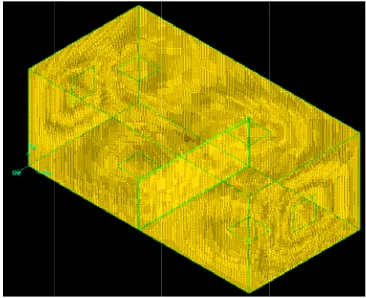
w of the model room
tilinear elemen g an elementa esults in a total dency check i oblem, the mes
of 2956750 fin he original me ing results pre
sh for the model r
that must be the turbulent mesh resolution an eddy viscosi
y algebraic mo solution of the
this investigati nd 38 cm respe ct is created as iddle of the roo ve through the mometer, a slot
th holes of 6 sensor probe th ctual experime for the validati
(b) Model
m geometry
nts, distributed l volume size l number of 87 is performed t sh is further re nite volumes). esh and the ref esented below
oom geometry
modeled. As motions of all n, the LES solu ity approach fo odels, such as t e high-frequenc
ive study is il ectively. In ord s shown in Fig. om. Air is allo other ceiling of 100 cm x 3 mm at every hrough a hole, ental model is s
ion for intende
Duct
uniformly, is of 0.6 cm x 0 70587 finite vo to assess the n efined to an el
The difference fined mesh is are obtained
opposed to th l scales, the LE ution can be ve or the descriptio
the Smagorinsk cy resolved flo
llustrated in Fi der to ensure th
.1(b). Within th owed to enter th outlet vent. F cm is created 10 cm. Durin , other holes a shown in Fig. ed configuratio
allocated for th 0.6 cm x 0.6 cm olumes generate
numerical erro lemental volum e in the air pha
found to be le with a mesh a
Th the one en found to b computatio volume me QUICK sc energetic e errors [11] Upwind-bi For pressu very low R combines a mesh is req Therefore, Convergen when the it
6 Experim
Hot-sphere temperatur m/s. The measuring Since the p It is difficu Fo the inlet of model room M conditions concentrati Vel is obtained redistributi
7 Model V The simula magnitude 6.0 [13] ar vertical lin
he vertical inle nd and exit vel
be 0.3 m/s an ons are perform
ethod. For RA cheme is used eddies that exi ]. The contribu iased schemes ure-velocity co Reynolds numb
a two-layer mo quired to resol
a wall model, nce for the airf
teration residua
mental Test Pr
e anemometer re in the model anemometers
error for air t probe size is la ult to estimate t or flow visuali f the model an m. However, it Measurement ar for more tha ion.
ocity at the inl d by fan fixed a
ion and uniform
Validations Ag ated air velocit along the hori e validated aga ne (Line 1) at in
et velocity of m locity is measu nd characterist med in steady ANS approach d to approxima ist near the cu ution of the LE
[12] and hence upling, the SIM ber, this study odel with enha lve the wall lay like the RANS flow governing
als are reduced
ocedures and
r has been us l room. For vel cannot reliabl temperature is arge (about 0.0
the error for ve ization, smoke nd flow of smo t is not ideal fo re conducted u an 3 hours b
let of the mode at inlet of the d m airflow befo
gainst Experim ty magnitude a izontal line at m ainst the measu nlet jet axis pr
model room is ured at desired tics length of
state condition employing th ate the convec ut-off wave nu
ES Subgrid Sc e the use of cen
MPLE algorith employs an en anced wall fun yer, which requ S approach, is g variables (ve d by five orders
Measuremen
sed for the m locity, the mea ly measure ve 0.4 K, includ 09 m in diame elocity fluctuat e of burning in oke is visualize or visualizing a under steady-s efore recordin
el room is taken duct model. Gu ore reaching the
Fig.
mental Results along the vertic mid-partition h ured results. Fi edicted throug
s determined b d end that will
0.1 m provid n. The transpo e standard k-ε ctive term at umber can sign ale force may ntral difference hm is employe nhanced wall t nctions, for the uires high com
used to bridge locity, pressur s of magnitude
t
measurements asurement rang elocity when t ding the errors eter), the probe tion.
ncense stick is ed which clearl airflow pattern state condition ng air velocity
n as the outlet v uiding plate acr
e diffuser outle
. 3 Experimental s
s
cal inlet jet axis height (line 2 in ig. 5 represents gh the two turbu
by using duct m be inlet to the des a flow Re ort equations ar ε a third-order the faces of t nificantly influ be overwhelm e scheme is ado ed. As the airf treatment, a ne e k-ε model. Fo mputational cos
e the wall with re, k and ε) is a e (e.g., 1 x 10⁻⁵
of air velocit ge of the hot-sp the magnitude introduced by es are sensitive
used. Burnin ly shows how in a particular ns by stabilizin y, air tempera
velocity of duc ross the main d et.
etup
s (line 1 shown n Fig. 4) obtain s the compariso
ulence models
model. An axia e room model. eynolds numb
re discretized interpolation the control vo uence the spati med by the use opted for the L flow near-wall ear-wall model or the LES mo st for engineeri the adjacent tu assumed to ha ).
ty, velocity fl phere anemome e is lower than y the data acqu e to high-freque
ng incense stick supply air is d area.
ng the room th ature, and vis
ct model that is duct is used to
n in Fig. 4) and ned by the CFD on of the air ve against the ex
al fan is fixed . The velocity er of 1500. A using the finit
scheme such olumes. In LE ial discretizatio e of Upwind an LES calculation l meshes can b ling method th odel, a very fin
ing application urbulent airflow ave been reache
fluctuations, an eters is 0.05 to n 0.10 m/s. th uisition system ency fluctuatio
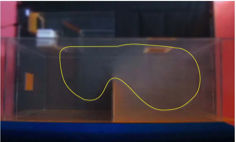
ks are located distributed in th
hermal and flu sualizing smok
s 0.28 m/s whic ensure the bett
Good agre LES turbul the distanc model, wh Fi horizontal location of the region results fou better than between th in this stud of the mod this it is o measureme sufficient f
eement has bee lence model. T ce 0.15 – 0.25 ich are neverth ig. 5 represen
line (Line 2) f x = 0m and th between x = 2 und in the regio n the LES mo he predictions a dy is that the L del’s inherent a
bserved that th ents. These m for the majority
en achieved be The results from
m. standard k heless also con nts the compar at the mid-pa he partition po 2 m and x = 4 on about the lo odel. Overall, and measured d LES model has
ability to bette he predicted v models can stil y of engineerin
Fig
etween experim m the LES mo k-ε model simu sistent with the rison of the pr artition height sition. Here ag
m. Marginal d ocation x = 0.8 both turbulen data and the fl shown to prov er capture the f velocities by th ll be applied w ng applications
g. 4 Defined locatio
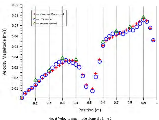
Fig. 5 Velocity ma
mental measure odel provides th ulation are slig e computer inv redicted and m t. Both models gain, the LES m discrepancy be 85 m shows th nce models pe ow trends are vide significant
fluid-flow cha he two k-ε mo with some deg s.
on for velocity me
agnitude along the
ement and num he best agreem ghtly under pre vestigations per measured air v s yields almos model provide etween the mea hat results obta erformed well; successfully ca tly better result aracteristics wit dels are still w gree of confid
easurement
e Line 1
merical predict ment in the mid edicted from th rformed by Po velocity comp st similar resu s a slightly bet asured data an ained by k-ε m good agreem aptured. One s ts especially in thin a confined within reasonab dence and are
tions by k-ε an ddle region fro
hose of the LE sner et al. [14] ponent along th
ults between th tter prediction nd the simulatio model are slight
ment is achieve ignificant aspe n zone 2 becau d space. Despi ble limits of th
C Fig. 7 and
omputational r Fig. 8 respecti
results using st vely.
Fig. 7
Fig. 6 Velocity ma
tandard k-ε mo
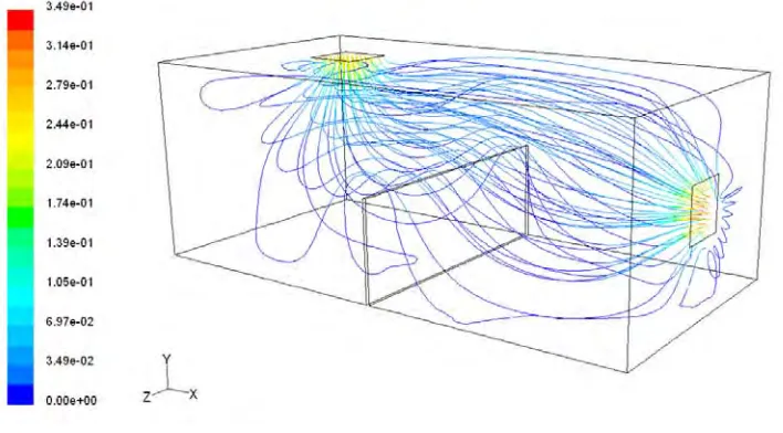
Velocity vector of
agnitude along the
odel in terms of
f air distribution in e Line 2
f velocity vecto
n model room
Fig. 8 Streamlines of air distribution in model room
8 Flow Visualization Using Smoke
There has been a great interest throughout the history of fluid dynamics, in making flow pattern visible. Flow visualization is a technique in which the flow conditions are determined by visual observation instead of being deduced indirectly from instrument readings. Flow visualization techniques are capable of yielding a macroscopic, though in many cases qualitative picture of the overall flow field [15]. This should be done in such a way that visualization technique does not alter the flow phenomena being visualized. These can be used to establish whether the flow is steady or fluctuating, laminar or turbulent, attached or separated; to indicate fluid particle paths, filament lines, or streamlines (lines everywhere tangent to the velocity vector). Smoke-flow visualization can thus reveal the entire flow pattern around a body. Ideally the density of smoke particle should be same as that of fluid. If density is different then the path of fluid and smoke differ appreciably because their gravitational and inertial forces are different. Smoke has slightly greater density than air. This makes it move outwards if streamlines are curved, and at low speeds smoke descends appreciably under the action of gravity. These effects are generally not serious if due care is exercised. In laminar flow the smoke filaments remains well defined but it diffuse very rapidly in turbulent flow. Best results are obtained at low velocities.
9 Observations and Conclusions
Fig. 9 Flow Visualization Using Smoke
Nomenclatures
Symbol Description
k Turbulent kinetic energy
V Velocity
u, v, w instantaneous velocity of air in x, y and z
directions
x, y, z Abscissa and ordinate of rectangular Cartesian
coordinate system
Greek Symbols
ε Turbulent kinetic energy dissipation rate
α Thermal diffusivity (k/ρcp)
μ Dynamic Viscosity
μt Turbulent viscosity
ρ Mass density
ν Kinematic viscosity (μ/ρ)
Superscripts
- Time-averaged value
’ Fluctuating value
References
[1] Sinha, S. L.Numerical Simulation of Room Airflow, PhD Thesis, Indian Institute of Technology, Kharagpur, (2000). [2] Mayinger, F. (1994). OpticalMeasurements:Techniquesand Applications (Springer,New York).
[3] Kähler, C.; Sammler, B.; Kompenhans, J.“Generation and control of tracer particles for optical flow investigations in air.” Experiments in Fluids 33 (2002) 736–742
[4] Patankar, S. V. Numerical Heat Transfer and Fluid Flow, McGraw Hill, Washington, (1980).
[5] Yao, J.; Jameson, A.;Alonso, J.; and Liu, F. “Development and Validation of a Massively Parallel Flow Solver forTurbomachinery Flows,” AIAA Paper No. 00-0882, (2000)
[6] Ferzinger, J. H. New Tools in Turbulence Modelling, Springer, New York, Les edition physique, Chap. 2, pp. 29-47, (1996). [7] Sagar, P. Large Eddy Simulation for Incompressible Flows, 2nd Edition, Springer, Berlin, (2002).
[8] Smagorinsky, J. “General Circulation Experiments With the Primitive Equation, I. TheBasic Experiment,” Mon. Weather Rev., 91(3), pp. 99-152, (1963).
[9] Germano, M.;Pionelli, U.;Moin, P. and Cabot, W.A Dynamic Subgrid-Scale Eddy Viscosity Model, Phys. Fluids A. 3(7), pp. 1760-1765, (1991).
[11] Park, N.;Yoo, J. Y. and Choi, D. Discretization Errors in Large-Eddy Simulation on the Suitability of Centered and Upwind-Biased Compact Difference Schemes, J. Comp. Phys., Vol. 198, 580-616, (2004).
[12] Mittal, R. andMoid, P. Suitability of Upwind-Biased Finite Difference Schemes for Large-Eddy Simulation of Turbulent Flows, AIAAJ, Vol. 35, 1415, (2007).
[13] FLUENT 6.0 Reference Manual, (1995).
[14] Tian, Z. F.;Tu, J. Y.;Yeoh, G. H. and Yuen, R. K.On the numerical study of contaminant particle concentration in indoor airflow, (2004).