Estimating Financial Volatility with High-Frequency Returns
Long H. Vo∗
Abstract: The primary value of a time series model lies in its ability to provide reliable
approximations of the modelled variable, both in-sample (where data are used to estimate model parameters) and out-of-sample (where the model is updated with new information and produces forecasts). In this paper, an overview of the various models in the GARCH family is followed by their application in estimating the daily volatility of Citigroup Inc., a major player in the US sub-prime mortgage crisis. Fitting these estimates to the ex-post realized volatility measure constructed from high-frequency returns provides superior goodness-of-fit than fitting them to the conventional absolute returns measure. This suggests that when modelling latent financial volatility, information revealed by high-frequency data can greatly enhance GARCH estimates’ performance.
Keywords: Realized volatility, GARCH models, frequency domain analysis, high-frequency
data.
Introduction
Poon and Granger(2003) emphasis the role of volatility in modern finance literature. The importance of volatility is apparent in a large variety of disciplines, of which the follow-ing are but a few: derivative pricfollow-ing (e.g. option pricfollow-ing depends heavily on underlyfollow-ing stock’s volatility), risk management (volatility forecasting has become crucial to determin-ing Value-at-risk especially after the global implementation of the first Basel Accord in 1988) and policy making (which relies on estimates of financial vulnerability via proxies of risk such as volatility).
Understanding the nature of volatility is therefore becoming ever more crucial in finan-cial modelling. Taylor (2005) proposed one of the most popular definitions of this variable: it is defined by standard deviation of a historical set of returns {rt|t = 1, . . . , T} whose
mean is ¯r= ˆµ= 1 T
T X
t=1
rt. The formula is thus:
σ=
v u u t
1 T −1
T X
t=1
(rt−r¯)2 (1)
∗Faculty of Finance, Banking and Business Management, Quy Nhon University, Binh Dinh, Vietnam.
Simply put, the volatility of an asset is the standard deviation of the returns on that asset away from its equilibrium (long-run mean) over a period of time (Hull,2006). In the finance literature, volatility is commonly measured by the absolute value of the returns. Though statistically improper, absolute value provides the best estimate of the standard deviation of a single return at a single period (Taylor,2005;Boubaker & Raza,2017).
As volatility captures the variability in asset prices, it is generally taken as a proxy for risk. Poon and Granger(2003) examine volatility via the continuous time martingale that generates instantaneous returns:
d(lnpt) =σtdWp,t (2)
where pt is the stock price and dWp,t denotes a standard Wiener process. In this
context, volatility can be thought of as a ‘scale’ parameter which adjusts the size of the variation associated with a stochastic Wiener process. Then, the conditional variance
of this return over the period [t, t+ 1] is called the ‘integrated volatility’:
Z 1
0
σ2t+τdτ.
Fundamental derivatives pricing theories were built upon this quantity under stochastic volatility (See for example Melino (1991), Hull and White (1996) and Hull (2006)). In general, σt is unobservable. However, if we can obtain a sufficiently large number of
continuously compounded returns over one time unit, the sum of the squared value of these returns shall provide us with a consistent estimate of the integrated volatility. This estimate is known as ‘realized volatility’.
Poon and Granger(2003) show that the accuracy of the realized estimate increases with the number of returns (or the sampling rate) computed at higher frequency. Proof of this proposition can also be found in (Barndorff-Nielsen & Shephard,2002;Chen, 2014). This means that given high-frequency data availability, the latent volatility process is plausibly observable. Beside being an ‘error-free’ volatility estimator, realized volatility is relatively simple to compute. A number of studies illustrated the importance of volatility measures constructed from returns recorded at high frequencies (See e.g. (Andersen & Bollerslev, 1998;Andersen, Bollerslev, Diebold, & Labys,1999) among others).
As the name suggested, high-frequency financial data are recorded much more fre-quently than the ‘standard’ data (e.g. daily data). Traditionally, the data used in pub-lished studies of financial time series analysis are both low-frequency and regularly spaced, while availability of high-frequency data has not resulted in a comprehensive literature until recently. This is due to the fact that low sampling rate of data can help reduce the costs of collection and storage significantly, and the equally spaced data points made it simpler to developed statistical inferences, though with limited confidence (Dacorogna, Gen¸cay, Muller, Olsen, & Pictet,2001). Incidentally, most high-frequency data are based on information arriving randomly and directly from markets, such as quoted prices from intraday transactions. This feature makes it very difficult to study these data using meth-ods that are designed for analysing equally spaced time series. On the other hand, one critical advantage introduced by huge influxes of high-frequency information, in terms of goodness-of-fit tests, is we can readily reduce the number of testing specifications1. This
is because statistical uncertainty decreases as the frequency of observations rises (Muller et al.,1995). In this paper, using returns computed from a unique set of high-frequency data, we shall illustrate the distinct advantage of these data in obtaining more precise estimates of realized volatility.
The rest of the paper is organized as follows: Section 2 discusses the importance of high-frequency data in greater details and introduce several ‘stylized facts’ of high-high-frequency returns. Section 3 introduces some popular models in the Generalized Autoregressive Conditional Heteroskedasticity (GARCH) family. Section 4 examines and compare the stylized facts of financial returns computed from both daily and intradaily data. Section 5 fits the GARCH model to our daily data and discuss the goodness-of-fit in-sample.
Section 6 demonstrates the improved performance of GARCH out-of-sample when we use a realized volatility measure constructed from high-frequency data. In addition, new evidence from multi-scale analysis suggests our wavelet decomposition may provide a better way of approximating the true volatility factor. Section 7 gives some concluding comments.
The Importance of High-frequency Data
Improvement on Volatility Estimates
Another important aspect of intraday data is that they can be used to investigate the difference in the dependence structure of volatility at different frequencies. In some cases, such as in a GARCH (1,1) model, inter-temporal aggregation is theoretically proved to be able to preserve volatility structure (See Drost and Nijman (1993)). However, empirical evidence generally suggests otherwise: volatility modelled at high frequencies exhibits much stronger persistence than at low frequencies Diebold(1988). This notion is, in principle, in line withNelson(1991) and is supported by Glosten, Jagannathan, and Runkle(1993), whose main finding is that persistence in volatility seems to diminish significantly when moving from daily to monthly data. Likewise,Andersen and Bollerslev(1997) argued that the long-memory behaviour observed in daily data also characterizes the volatility process at high frequencies, after filtering out all intraday dependencies.
With regard to the examination of high-frequency stylized facts,Andersen and Boller-slev(1997) noted the sharp contrast between the highly dependent dynamic in daily volatil-ity to a less profound long-term dependence among intraday volatilvolatil-ity. According to these authors, the seemingly contradictory evidence of volatility persistence in daily and in-tradaily data is attributable to the fact that intraday volatility can be regarded as“[The] aggregation of numerous constituent component processes; some with very short-run decay rates [which dominate in intraday returns] and others possessing much longer-run depen-dencies”. In turn, the multiple volatility components at the intradaily frequencies are a result of numerous heterogeneous information arrival processes. From a different angle, Jensen and Whitcher (2000) capture the presence of both short and long-memory (as a result of unexpected as well as anticipated news) with a non-stationary, but locally station-ary, stochastic volatility estimator. Their primary finding is a time-varying long-memory parameter which exhibits an intradaily pattern: being highest and lowest in accordance with the opening and closing of foreign exchanges. These authors open up the debate of whether this strong time-of-the-day effect is caused by public macroeconomic news an-nounced at the beginning of some markets, or the capitalization of informed traders at the end of other markets. In any case, the link between volatility dependence structure and the pattern in which new information arrives is central in understanding market op-erating dynamics. Furthermore, the evidence that long-memory parameter peaks at the close of most active trading exchanges documented by Jensen and Whitcher (2000) and heterogeneous volatility structures captured byAndersen and Bollerslev(1997) both point to the association between the persistence of volatility and less active, less volatile trading sessions.
The Stylized Facts of High-frequency Financial Returns
The most notable fact of financial returns is perhaps the Non-normal (or Non-Gaussianity) or the heavy tailed distribution. Earlier empirical analyses dated as far back as the 1970s had repeatedly placed much emphasis on documenting related visual features and numerous implications of returns’ distribution such as its approximate asymmetry, the heavy tails and its high peak (see, for example, (Mandelbrot,1963;Fama,1965).
variations in their orders and wordings, we believe it is helpful to list the propositions in group of ‘traditional’ categories, namely: facts about distributions, autocorrelations, seasonality and scaling properties:
• The middle price is subject to microstructure effects at the highest frequency
• Intraday returns exhibit distribution with heavy tails, with increasing kurtosis pro-portional to increase in observation frequency
• Intraday returns from traded assets are almost uncorrelated, a part from a significant first-order correlation
• There exists seasonal volatility clusters distinctive to different days of the week
• There exists short bursts of volatility following arrival of major macroeconomic news
Our main interest is placed on the long-memory property exhibited by measures of daily and intradaily volatility. Poon and Granger(2003) assert that slow decay autocorre-lation of variances is a very well-established stylized fact throughout the literature (refer to Granger, Spear, and Ding(2000) for further reviews). According toAndersen and Boller-slev(1997), long-term dependency is an inherent characteristic of the underlying volatility generating process. These authors also attribute the inconsistent conclusions about the level of volatility dependence to the fact that volatility process is actually a sum of multi-ple components. Volatility estimates are therefore affected by either short-run components (when using high-frequency data) or long-run ones (when using daily data). However, with appropriate restrictions imposed, the aggregated volatility process always exhibits long memory. Christensen and Nielsen (2007) and Fleming and Kirby (2011) as well as many academics having experience in the field agreed upon the feasibility of describing re-alized volatility with a fractionally integrated process where the long memory parameterd is within the range of 0.3 - 0.5. However, they also documented short-lived modest impacts of volatility changes on stock prices. In any case, volatility long-run dependence structure possesses a complex nature.
An important question is that what makes the existence of long range dependence crucial to studies of financial time series? One problem with the classical asset pricing theories is pointed out by Lo(1991): whenever such dependence structure exists among financial returns, the traditional statistical inference for tests of the capital asset pricing model and the arbitrage pricing theory, both of which rely on a martingale returns process, is no longer valid. Furthermore, the larger the long-memory effect, the greater the impact of shocks on future volatility. In practice, however, financial returns are almost always observed to be uncorrelated and thus exhibit very little long-run dependence.
Modelling Volatility with the GARCH Family
of volatility models that enjoy vast popularity among academics, namely: the GARCH family models and the stochastic volatility models. While the former studies volatility as a function of observables, the latter incorporates not only observables, but also unobservable volatility components (See (Taylor, 2005) for a review of the topic). For our purposes, it is sufficient to study the first branch, which originates from the introduction of the Autoregressive Conditional Heteroskedastic (ARCH) model first proposed in the seminal paper of (Engle, 1982). This model is designed to capture the time-varying nature of conditional volatility given the historic information of returns. It is important to note that stylized facts of volatility serve as theoretical motivations of specific extensions of the ARCH model. The paper byEngle and Patton(2001) reviews major stylized facts of volatility that should be incorporated in a good model. Specifically, these facts include: (i) volatility clusters, (ii) persistence, (iii) mean reversion and (iv) asymmetric impacts of innovations. Unable to cover the enormous body of research on this model family, our paper only investigates the frameworks most directly designed to incorporate these four stylized facts. Next we shall discuss the salient specifications and their relevance to our research in more detail.
Following the traditional approach we define the one-period continuously compounde-d returns as the first order difference of the natural logarithm of a discrete price sequence. AsTaylor(2005) argued, the number of dividend payment days is very small compared to the sample of trading days and thus dividend can be ignored in this setting:
rt= ln(pt)−ln(pt−1) = ∆ln(pt) (3)
Assuming that asset returns are generated by the following process2:
rt=µt+σtzt where zt∼i.i.d N(0,1) (4)
in whichµt|t−1=Et−1[rt] andσt|t−1=Et−1[(rt−µt)2] are the process’ conditional mean
and variance respectively, given the information set at timet−1 (which is the set of returns up tot−1, inclusive).
We also specify the ‘residual returns’ asut=rt−µt=σtzt. Note that the conditional
meanµt tends to be modelled as an ARMA process in some contexts in order to free the
residuals of serial correlations. Nevertheless this variable is usually set to zero or constant 3, as over the long term, in a large sample the average returns tend to be insignificant
(Taylor,2005)4. The (population) unconditional mean and variance can be defined as:
µ=E[rt] and σ2=E[(rt−µ)2] (5)
2This is the standard specification of all ARCH-type models examined in this paper. Therefore we
implicitly assume it in most of the later discussions.
3In general there are three specifications for conditional meanµ
t: we can treat it as zero, a constant, or
adding an ARCH term determinant (meaning the expected value of returns also depends on past evaluation of volatility). The last type is commonly referred to as the ARCH-in-mean or ARCH-M model. The difference only results in different forecast of returns while not affecting our main interest - the volatility estimates - in any significant way.
4Which is why the residual returns (or ‘de-meaned’ returns) and original returns series have similar
As the name suggests, ARCH models conditional volatility auto-regressively, meaning fu-ture volatility is specified to be linearly dependent on immediate previous squared residual returns. In other words, large/small deviations from mean return is followed by high/low subsequent variances. This allows us to effectively capture volatility clustering feature and is one of the reasons for the original success of the ARCH-type model:
σ2t =ω+α(u2t−1) (6)
with ω >0, α >0. This is the simplest form of ARCH: the ARCH(1) model. When we increase the number of autoregressive terms top, we have its extended form: the ARCH(p) model5:
σ2t =ω+
p X
i=1
αiu2t−i (7)
AsCampbell, Lo, and MacKinlay(1997) pointed out, setting volatility to be time-varying allows us to capture basic stylized facts of financial returns, most notably the property that returns’ distribution is heavy tailed with excess kurtosis.
In this case the returns process is stationary only if
p X
i=1
αi<1 (withαi>0∀i) so that
it has a finite long term unconditional variance, which can be computed asσ2= Var(u
t) =
ω 1−Ppi=1αi
. Also, the ARCH process is then mean-reverting.
The GARCH (1,1)
Despite its inherent ability to capture volatility clustering, ARCH model fails to account for volatility persistence, as the clusters are short-lived without accounting for extra lagged ut terms. Bollerslev (1986) augmented this model by adding a lagged term of
condi-tional volatility, forming the Generalized Autoregressive Condicondi-tional Heteroskedasticity (GARCH) (1,1) model6:
σ2
t =ω+α(u2t−1) +βσt−2 1 (8)
where ω > 0, α > 0, β > 0 and α+β < 1. It can be shown that the GARCH (1,1) is analogous to an ARCH(∞) 7. The GARCH (1,1) inherits its predecessor’s ability to capture the excess kurtosis of returns’ distribution. Furthermore, the most important
5pis also known as the lag parameter in this context.
6Also, ARCH model is analogous to an AR model on squared residuals, whilst GARCH can be thought
of as an ARMA model on squared residuals.
7By recursively replacing the past volatility terms with their GARCH forms we can write the GARCH
model as:
σ2
t =ω+αu2t−1+βσ2t−1
=ω+αu2
t−1+β(ω+αu2t−2+βσ2t−2) =· · ·= ω
1−β+α/β
∞
X
j=1 βju2t−j
application of this model is its ability to forecast future volatility. We have the l-ahead volatility forecast specified via:
ˆ
σ2t+l=σ2+ (α+β)l(σ2t−σ2) (9)
Here the term (α+β) is known as ‘persistence parameter’ as it determines the rate at which the variance forecast converges to the long-run unconditional varianceσ2=E[u2
t] =
ω
1−(α+β)when the forecast horizon tends to infinity (l→ ∞). To describe this particular implication of GARCH,Engle(2001) stated that “the GARCH models are mean reverting and conditionally heteroskedastic, but have a constant unconditional variance”(p.160). This is an important complement of GARCH to ARCH. A related quantity specifying the degree of volatility persistence is the ‘half-life’, denoted ask. It is the time needed for the variance to move halfway towards its unconditional level. Generally we have (α+β)k = 0.5 or
k= ln(0.5)/ln(α+β). For the GARCH model to be stationary we must have (α+β)<1. We can write the generalized form of this model as:
σ2t =ω+
p X
i=1
αiu2t−i+ q X
j=1
βjσ2t−j (10)
For the sake of tractability we only focus on the simple GARCH (1,1) as well as its related models with the same ARMA order from here on. Many researchers strongly suggest the comparability of such simple models to the ones incorporating higher order ARMA terms. Furthermore, it is widely documented that GARCH (1,1) generally equals or rivals other, more complex models in the same family, especially in terms of out-of-sample forecast performance (SeeHansen and Lunde(2005)).
Data
Our main focus in this section would be to provide a preliminary investigation on Citi-group’s stock prices and returns over the last 30 years or so. Here, we explore some pre-liminary analyses of daily returns and volatility, with emphases on the so-called ‘stylized facts’, specifically the heavy-tailed distribution and the autocorrelation structure. Detailed description of this company and its role in the Global financial crisis is provided in Ap-pendix A. This is followed by description of our transformation of daily prices into returns in Appendix B.
Stylized Facts of Returns
We collect daily closing prices of Citigroup between 03 Jan 1977 and 31 Jul 2013 from
of Citigroup’s closing price and closing price adjusted for stock splits and dividend, as well as their corresponding returns series (computed by concatenating method). Some most notable features of these series are: (i) the price spikes just before 1998 (the year of the merger between Citicorp and Travelers Group) and exhibits some volatility before continuing to grow; (ii) there are two other major falls of the stock, corresponding to the 2000s Internet bubble bust and Enron scandal (2002) as well as the recent GFC (about right after the rescue package the firm received); (iii) the huge downward trends lead to the most volatile period in returns from 2008 to 2010. In addition, when comparing the closing and adjusted closing price series, a very strong impression is the extremely different scales on the two graphs. In subsequent analyses we shall focus on the ‘adjusted’ returns time series, in which the definition of one-period continuously compounded returns is established as in Section 3, wherePt is the adjusted closing price at timet, i.e. rt= lnPt−lnPt−1.
Asymmetric Impact of Returns on Volatility
A stylized fact that is widely documented in quantitative finance researches is the neg-ative correlation between stock returns and their volatility. This phenomenon is largely attributed to the changes in leverage ratio corresponding to changes in stock prices. In particular, a fall in stock price generally has a much larger impact on volatility than a rise of the same magnitude, since it causes the debt-to-equity ratio to rise, thus provoking equity investors’ concern about their claim in the firm. We can illustrate this feature by plotting the stock prices against corresponding absolute returns (as a conventional proxy for volatility):
For the period from 1977 to 2008 the increase in share price results in relatively low level of volatility that is distinct from that of the period from 2008 to 2010. From Figure 2 we can see clearly the inverse direction/sign exhibited by stock returns and volatility: whenever prices go down, volatility goes up and vice versa. Furthermore, the impacts of positive and negative price changes on volatility are dramatically different: a steep rise from 1995 to mid 2007 (indicated by the green trend line) results in a change of volatility that has roughly the same magnitude as the change corresponding to the period from mid 2007 to 2009 (indicated by the red trend line). In other words, the strong fall during the three years of GFC undid the gain built up in previous 12 years and was undoubtedly related to one of the most volatile, unprecedented periods in the history of the finance world. Aside from this obvious feature, the asymmetric relation between price changes and volatility is repeated throughout Citigroup’s timeline.
This relationship was explicitly studied via the specification of asymmetric GARCH models earlier. It will be further elaborated at different time horizons in later sections via the investigation of the leverage effect hypothesis.
On the other hand, looking at Figure 2 one can argue that the relationship between the direction of price movement and the magnitude of volatility can be somewhat expected and the above argument about impact of the sign is not necessarily applicable. The reason is that if we consider volatility to be proportional to the absolute value of the quantity
∆P
to the slope of the trend lines associated with these periods. The longer the period, the smaller the slope (in terms of absolute value) and vice versa.
Figure 1
Time series plot of Citigroup daily data. From top to bottom: close price, returns (close-to-close), adjusted close price, returns (adjusted close-to-adjusted close). Data range from 03 Jan 1977 to
31 Jul 2013.
Figure 2
Comparison between Citigroup daily price series (adjusted for stock splits and dividends) and the corresponding absolute returns series, for the period 1977-2013. The two red ovals indicate periods when visible sharp price drops corresponding to high volatility (aside from the drop in the GFC).
However, we do not observe the relationship in a reverse order, i.e. bullish trend lines having greater slope, thus without a ‘counter-factor’ we can not verify whether or not the direction of price changes is really unimportant. In any case, the observation of asymmetric impact of price changes remained relevant, at least in our sample period.
Long-run Autocorrelation
illustrated by the absolute series. To better clarify this fact, we plot the autocorrelation function for the returns series together with its squared and absolute series in Figure 3.
For the returns series, although it is difficult to observe the overall significance of the ACF, the Ljung-Box portmanteau test (reported in Table 1 in the next subsection) indicates there is serial correlation among returns up to lag 21, implying our empirical returns are not independent. For the volatility series, we can clearly see the hyperbolic decaying ACFs of the squared and absolute returns which retain their high significance as far as lag 400. This feature implies the long run impact of present shocks to returns on future returns, and must be taken into account when modelling volatility.
Furthermore, when we increase the lag range, we observe a more visible hyperbolic decaying pattern of the ACF functions of squared returns and absolute returns. This indicates a long-memory behaviour of these processes. This feature implies the long run impact of return shocks, which must be taken into account when modelling volatility.
The Leptokurtic Returns Distribution
A common feature of the distribution of financial returns (or residual returns) is its exces-sive kurtosis relative to a Gaussian distribution (whose theoretical kurtosis is 3). In other words the fourth central moment of these variables is usually greater than 3, implying a heavy-tailed distribution. To illustrate, we plot the histogram of the standardized returns
Zt =
rt−r¯
s where ¯r and s are the sample mean and standard deviation of returns, re-spectively. When compared with other distributions such as the Gaussian, the Student-t (with degrees of freedom of 10) and the Generalized Errors Distribution (GED) we see that the distribution of our standardized returns exhibit excess kurtosis and slightly negative skewness, as shown in Figure 4.
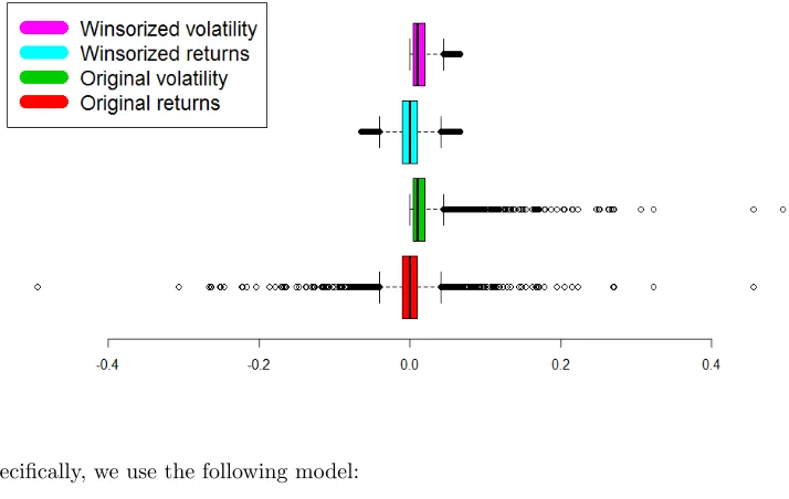
We also note that since the fourth moment raises the variation to a power of four, it is very sensitive to extreme fluctuations of returns around the mean. Therefore, when ex-amining kurtosis, it is desirable to winsorize our data, to make the empirical implications less susceptible to outliers. In particular, we truncate the extreme returns smaller than the 1% quantile and greater than the 99% quantile and consider these as outliers representing impacts of market crashes. Then we replace the negative extreme values by the 1% quantile and the positive extreme values by the 99% quantile. From Figure 5, when studying the boxplots of the 4 time series we can clearly tell the significant reduction of outliers when replacing the ‘raw’ data with winsorized data.
Figure 3
Correlograms of Citigroup daily time series for the period 1977-2013, up to 1000 lags. The blue dashed lines indicate the 95% confidence intervals.
The summary statistics of the raw returns (denoted as rraw) and winsorized returns
(denoted as rwins) time series along with their corresponding volatility proxies (absolute
returns) are reported in Table 1. The distribution of standardized winsorized returns, viz. rwins, still exhibits robust excess kurtosis compared to a standard normal distribution.
Figure 4
Histogram of standardized daily Citigroup returns for period 1977-2013, with lines indicating the fitted normal, student and GED density functions superimposed.
Test for Unit Root Non-Stationarity
It is observed that unit root non-stationary time series often exhibit slow decaying ACFs similar to those of stationary long-memory processes. Therefore it might not be possible to distinguish the two type of processes relying only on the ACF (Brooks,2002). To find out whether our time series are non-stationary, we apply the Augmented Dickey-Fuller (ADF) test for unit root (seeDickey and Fuller(1979) andHamilton(1994)).
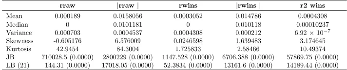
Table 1
Summary statistics for Citigroup daily data for the period 03 Jan 1977 to 31 Jul 2013
rraw |rraw| rwins |rwins| r2 wins
Mean 0.000189 0.0158056 0.0003052 0.014786 0.0004308
Median 0 0.0101181 0 0.010118 0.00010237
Variance 0.000703 0.0004537 0.0004308 0.000212 6.92×10⁻⁷
Skewness -0.605176 6.576009 0.0246598 1.639483 3.174645
Kurtosis 42.9454 84.3004 1.725833 2.58466 10.49374
Figure 5
Boxplots of daily time series of Citigroup for period 1977-2013. The black line indicates the median. The number of outliers (or the length of the whiskers) is reduced significantly with the winsorized data. Here the width of the boxes represents the Interquartile Range (IQR), or the difference between the upper quartile-UQ (or the 75% quantile) and lower quartile-LQ (or the 25% quantile). The lower and upper
‘whiskers’ indicate the values equalLQ−1.58×IQRandU Q+ 1.58×IQR, respectively. See e.g.McGill,
Tukey, and Larsen(1978) andChambers, Cleveland, Kleiner, and Tukey(1983). Any value falling outside of the range implied by these whiskers is considered an outlier.
Specifically, we use the following model:
∆(Xt) =α+βt+γXt−1+
p X
i=1
δi∆(Xt−i) +t
Hereαis a constant andβ is the coefficient of the time trend. Including both coefficients allow us to test for unit root with a drift and a deterministic time trend simultaneously. Unlike the original DF, the ADF adds the lagged differenced terms to account for up to order p serial correlation in the data generating process which could invalidate the statistical inference of DF test. The ‘optimal’ number of augmenting lags (p) is determined by minimizing the Akaike Information Criterion. ADF test statistic is the t-stat of the OLS estimate ofγ. The null hypothesis of ADF test isγ = 0. Intuitively, when γ = 0 is not rejected, the time series is not stationary, and the lagged level (Xt−1) cannot be used to
predict the lagged change (∆(Xt)).
Table 2
Augmented Dickey-Fuller test for stationarity in daily time series
Null hypothesisH0:γ= 0
Test Eq. Series ADF stat Critical value*
Returns -67.142 1% -3.4593 Squared returns -45.963 5% -2.8738 Absolute returns -46.95 10% -2.5732 (*) The critical values are obtained from MacKinnon (1994)
In-sample Performance: Volatility Estimate with GARCH
Models
We continue with analyses of GARCH frameworks covered in the previous sections, using the daily returns of Citigroup Inc. computed from the time series of closing prices, which are adjusted for stock splits and dividends. We use 7341 observations from 01 Dec 1977 to 31 Dec 2006 and refer to these as our in-sample data.
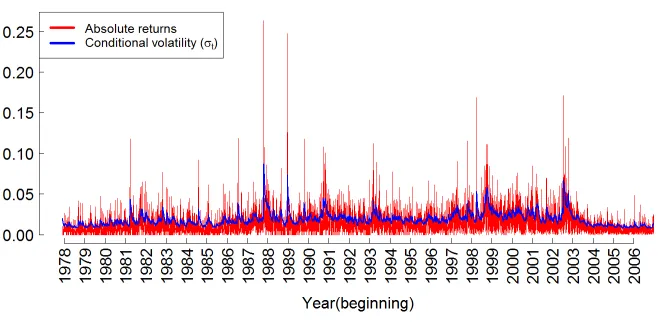
To illustrate the goodness-of-fit of GARCH(1,1), we first plot the fitted conditional volatilityσt(formulated in previous sections) against in-sample absolute returns in Figure
6. As can be seen, the overall shape ofσb2t tracks that of the actual data quite reasonably,
save for the extreme values observed at several market crashes.
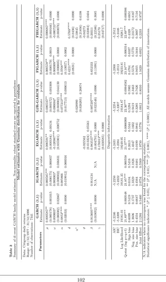
Comparing Models’ Performance
Model estimates and Diagnostic statistics are reported in Table 38. Most of the estimated parameters are significant. The portmanteau Ljung-Box tests (up to lag 21) suggests no evidence of serial correlation among model residuals, indicating that these models seem to perform adequately. Interestingly, the EGARCH(1,1) yields the highest value of Log-likehood function compared to other GARCH models previously discussed, as well as the lowest value of Akaike Information Criterion (AIC)9. Both of these indicators imply better performance of EGARCH. It should be noted that the FIGARCH(1,1) ranks second in terms of performance and yield a estimated d= 0.4221 (corresponding to a Hurst index of 0.9221) which is significant at the 1% level. Taken together, the improved performance of EGARCH and FIGARCH imply that our volatility series does exhibit (i) a high degree of long-memory and (ii) an asymmetric relationship with positive and negative returns. Inspired by these findings, we opt to specify yet another class of GARCH model designed to incorporate these two properties of financial volatility. The new model is called the Fractionally Integrated Exponential ARCH (FIEGARCH), which was first proposed in Nelson(1991) and then further examined byBollerslev and Mikkelsen(1996).
8All estimates are obtained with the help of R packagerugarchGhalanos(2013), except for the results
of FIGARCH and FIEGARCH (which are obtained using OXMetrics (Laurent & Peters,2002).
9In its general form the AIC is defined as :AIC= 2k−2ln(L) wherekis the number of model parameters
andLis the maximized likelihood value of the estimated model (Akaike,1974). For comparison, the model
Figure 6
Fitting GARCH (1,1) model. In-sample data range from 01 Dec 1977 to 31 Dec 2006
Similar to the nesting of GARCH under FIGARCH, by incorporating the fractional or-ders of integration to EGARCH, we effectively nest it under the FIEGARCH model which, by definition, also nests FIGARCH. In particular, from the specification of EGARCH in Equation 16 we factorize the AR polynomial as [1−ϕ(L)] =φ(L)(1−L)d and have:
ln (σ2t) =ω+φ(L)−1(1−L)−d[1 +ψ(L)]g(zt−1)
with g(zt−1) =ϑzt−1+γ(|zt−1|−E[|zt−1|])
(11)
Analogous to the EGARCH model, here ϑ <0 andγ >0 generally confirm the asym-metric impact of returns on future volatility. Apparently the superiority of FIEGARCH compared to EGARCH is the ability to account for long-memory, which is represented via the parameter d. When d = 0 this model reverts to conventional EGARCH. Bollerslev and Mikkelsen(1996) point out that the FIEGARCH process does not have to satisfy any non-negativity constraints to be well-defined. Fitting this model gives us a Log-likelihood 19281.7, which is even higher than that obtained with EGARCH. The fractional difference parameter is estimated at 0.58, which is significantly greater than 0.5 and is questionable. Finally, to quantify the model goodness-of-fit we simply regress the absolute returns against the fitted ˆσtvia the following Equation:
|rt|=a+b .ˆσt+ut (12)
and obtain the corresponding coefficients of determination: R2 = 0.12042, 0.12047,
low in-sampleR2is a result of persistent underestimation of the fitted ˆσt2compared to daily
volatility proxied by absolute returns (see Figure 6). This, in turn, may be a result of the presence of extreme volatility accompanying crises related to the 1980s housing bubble, the 1987 market crash, the 2000s Internet bubble burst or the 2008 global financial distress, for which GARCH failed to provide good estimates.
Diagnostic Residual Tests
Specifically, for GARCH(1,1) the Ljung-Box test for serial correlation yieldsQ(21) = 30.693 (p-value = 0.059) for residuals (zt) andQ(21) = 6.8541 (p-value = 0.997) for squared
resid-uals (z2t). This means we cannot reject the null hypothesis of no serial correlation for either
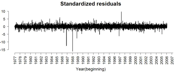
of these series at 5% level for even as far as 21 lags. Indeed, the pattern exhibited by the time series plot ofztin Figure 7 is analogous to that of a white noise process, and an
indi-cator of the appropriateness of our GARCH model (for similar analyses, seeTsay(2001), p.97):
Figure 7
Time series plot of standardized residuals of GARCH(1,1) Data sample from 01 Dec 1977 to 31 Dec 2006.
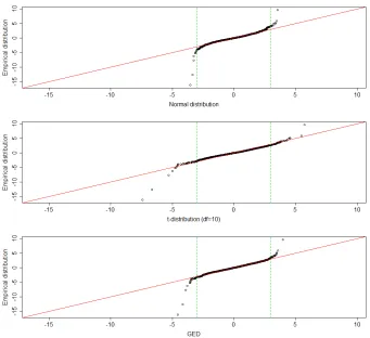
Another relevant test of residuals involves examining their distribution. Because one important assumption of our GARCH(1,1) model is that the innovationsztare
condition-ally normcondition-ally distributed, it is necessary to check if this assumption holds with model’s standardized residuals. Checking for normality can be done via inspecting histogram and Jarque-Bera test. Figure 8 indicates a leptokurtic distribution (with a excessive kurtosis of 18.35) and the Jarque-Bera test strongly rejects the null hypothesis of normality.
Non-normality is also visible through the quantile-quantile plot of the empirical dis-tribution ofzt against that of a Student distribution (with 10 degrees of freedom) and a
negative and positive returns shocks, which is consistent with the fact that GARCH (1,1) is unable to discriminate between the signs of shocks. Deviation from t-distribution and GED, on the other hand, seems to be mostly driven by large positive shocks.
Figure 8
Histogram and descriptive statistics of standardized residuals for GARCH(1,1).
Density curves from 3 distributions: normal, Student and GED with comparable mean and variance are superimposed.
Given these insights, we proceed to adjust our original assumption of normality and re-estimate the GARCH models with Maximum likelihood functions corresponding to the Student t-distribution and Generalized errors distribution (note that our original estimates are robust to non-normality thanks to robust standard deviation proposed by Bollerslev and Wooldridge(1992). Other conditions are preserved for estimation. Results are re-ported in Tables 4 and Table 5 for t-distribution and GED, respectively. Overall we observe improvement in terms of higher Log-likelihood values: for example, for GARCH(1,1) the maximum Log-likelihood increases from 19181.01 with Normal distribution to 19642.62 for t-distribution and 19587.99 for GED. Likewise the AIC decreases from−5.22 to−5.35 and −5.33. Estimated values of main parameters and corresponding significance do not change dramatically. However, this seemingly improved goodness-of-fit (with respect to empiri-cal returns data) is not manifest in increased R-squared from regressing absolute returns against ˆσ2
t. In particular, with GARCH(1,1) we obtainR2= 0.1202 for t-distribution and
R2 = 0.1200 for GED (compared to R2 = 0.12042 for normal distribution). However,
of this model in these two cases. Nevertheless, throughout the various specifications of residuals’ distribution, FIGARCH(1,1) exhibits a very high degree of fractional difference parameter (around 0.42).
Figure 9
Q-Q plots of residuals’ distribution against normal distribution (top), t-distribution (middle) and GED (bottom). Red line indicates identity line.
Out-of-sample Performance: Daily Volatility vs.
Real-ized Volatility
approach of Andersen and Bollerslev(1998) andHansen and Lunde (2005). In line with these authors, we find some evidence for the credibility of GARCH (1,1) model.
It should be noted that, throughout the section, we focus on ‘ex-post’ one-period-ahead forecasts when evaluating model performance out-of-sample, meaning we use known returns data to update our estimated GARCH model and get the forecasts of volatility (a technique known as ‘rolling forecast’). Although these forecasts have less practical value than the ‘ex-ante’ forecasts (e.g. rather than using known returns to get volatility forecasts, we may first forecast returns themselves), this is a standard approach which provides an objective and direct assessment of model performance.
Study Design
To begin, we use a more general notation of returns proposed byAndersen and Bollerslev (1998), which incorporates the sampling frequencym:
r(m),t=pt−pt−1/mwhere t= 0,1/m,2/m, . . .
in whichptdenotes the logarithmic price. Given the sampling ratem, we define{r(m),t}as
the discretely observed time series of continuously compounded returns withmobservations per day. The instantaneous returns process is then defined as rt ≡ r(∞),t ≡dpt. When
m= 1 we have the daily returns, which represents the standard frequency in many studies. FollowingAndersen and Bollerslev(1998) we model the (1-period) daily volatility using the generalized GARCH (1,1) specification:
σ2(m),t=ω(m)+α(m).r(2m),t−1/m+β(m).σ2(m),t−1/m
r(m),t=σ(m),t.z(m),t
where ω(m)>0, α(m)≥0, β(m)≥0 z(m),t∼i.i.d N(0,1)
wherem= 1
(13)
Theoretically, if we have a correctly specified model, our forecast must equal the true return variance, i.e.:
E(r2t+1) =E(|rt+1|2) =E(u2t+1)≡σˆ 2
t+1
This motivates a direct way to evaluate GARCH forecast performance, that is, to use some type of MSE (mean squared errors)-based metrics to test for the null hypothesis: E(ˆσt2+1−Var[rt+1]) = 0. To do this the most popular approach is analogous toMincer and
Zarnowitz (1969)’s method of evaluating conditional mean forecasts (but in this context we need to evaluate conditional variance forecasts instead). In particular, we simply need to regress some ex-post realized volatility measurement on the estimated values obtained from GARCH (1,1) as follows:
r2(m),t+1/m=a(m)+b(m). ˆσ(2m),t+1/m+u(m),t+1/m (14)
performance, because daily squared return is an unbiased, but very noisy estimator of the true latent volatility. This is evident in a ‘disappointingly’ low R-squared obtained when regressing this proxy on the forecasts, as commonly observed in numerous contemporary papers. In hope of reducing the degree of misspecification associated with using squared returns by a power of 2, we opt for using absolute returns. This is also consistent with the view of volatility as standard deviation rather than variance. In addition,Taylor(1986)’s findings suggest that better forecasts of volatility were provided by models using absolute returns compared to squared returns. This might be a result of absolute returns displaying higher degree of long-memory than squared returns, which motivates direct modelling of volatility from absolute returns (See e.g. Ding and Granger(1996) andVuorenmaa(2005)). Furthermore, as pointed out byVuorenmaa(2005), since the logarithmic squared value of a close-to-zero return would be negative, it is less favourable to be used as volatility proxy compared to an absolute return, which is more robust to this kind of ‘inlier’ problem. The above arguments have been largely verified with stock data, at the very least.
Application
We start with estimating the GARCH (1,1) model (specified in Equation 13), using in-sample data based on daily returns of Citigroup, Inc. from 01 Dec 1977 to 31 Dec 2006. Next, we update the estimated model with out-of-sample daily returns from 03 Jan 2007 to 31 Dec 2007 and get the rolling forecast of volatility (denoted as ˆσ(m),t+1/m). Consequently,
our one-step ahead GARCH(1,1) volatility forecasts are computed for the period of 250 working days of the year 2007 (excluding weekends and holidays for their insignificant trading activities). We then proceed to replace the fitted/forecast variance in equation 14 with these values. In other words we modify Andersen and Bollerslev (1998)’s approach by regressing absolute returns on forecast standard deviation instead of regressing squared returns on forecast variances10:
|r(m),t+1/m|=a(m)+b(m) .σˆ(m),t+1/m+(m),t+1/m (15)
Substituting absolute daily returns (m= 1) into this generalization we have:
|r(1),t+1|=a(1)+b(1) .σˆ(1),t+1+(1),t+1 (16)
The R-squared value of Equation (16) (R2
(1)) can be viewed as a simple indicator of how
well our estimates of volatility can explain the variability in the ex-post returns which, in theory, can not be observed. The problem remains, as discussed earlier, that traditional daily proxies of volatility (e.g. squared residual returns, squared returns, absolute returns) may not be adequate. In particular, as can be seen in Table 4, using daily absolute returns as volatility proxy (or the dependent variable in Equation 16) suggests that our GARCH(1,1) model only explains 13.9% of the daily variability of returns. When using
10The former specification is also adopted by (Jorion,1995). A viable alternative would be to compare
volatility forecasts with ex-post returns shocks (or residual returns) out-of-sample. But asTsay(2001)
argued, using returns shocks as a measure of realized volatility may not be a good idea. A single realization
of the random variableu2
t+1is not adequate to provide an accurate estimate of the movement of day-by-day
squared returns we obtain a decreased value: R2(1)= 0.0997, but this is still higher than the correspondingR2values reported inAndersen and Bollerslev(1998)’s exchange rate study, i.e. 0.047for the Deutsche Mark/U.S. Dollar (DM-$) and 0.026 for Japanese Yen/U.S. Dollar (U-$) rates.
All things considered, these results suggest that absolute returns may provide a more appropriate volatility proxy than squared returns. However, regardless of the proxies used, the low R2
(1) and a poor out-of-sample fit are to be expected, as both proxies are noisy
estimators of true volatility process. In defence of the GARCH model, Andersen and Bollerslev(1998) assert that the use of these noisy proxies distort our perception of GARCH forecasts performance, because “[...] Rational financial decision making hinges on the anticipated future volatility and not the subsequent realized squared returns. Under the null hypothesis that the estimated GARCH(1,1) model constitutes the correct specification, the true return variance is, by definition, identical to the GARCH volatility forecast.” (p.890).
Realized Volatility Proxy Constructed from Intraday Returns
The above arguments imply that to obtain meaningful forecast evaluation we first need to acquire a better volatility estimate. According to the theory of quadratic variation (See Karatzas and Shreve(1991)), in principle, the cumulative squared intraday returns provide better approximation to ex-post volatility at higher sampling rate:
limm→∞( Z 1
0
σt2+τdτ −
m X
j=1
r2(m),t+j/m) = 0 (17)
in which
Z 1
0
σ2t+τdτ denotes the continuous time volatility measure and r2
(m),t+j/m is
the lengthj/mperiod squared return. Motivated by this proposition,Hansen and Lunde (2005) show that when intraday returns are uncorrelated we have an unbiased estimator ofσ2
t simply by summing intraday squared returns:
ˆ σ2(m),t≡
m X
j=1
r(2m),t+j/m
Ehˆσ2 (m),t
i
=E(r2
t) =E h
ˆ σ2
(1),t i
(18)
For Citigroup Inc., millisecond-timestamped tick data are collected for the year 2007. The first and last tick of each day are omitted in this calculation, as their corresponding trading volumes are much higher than those of the rest of the ticks. These ‘outliers’ are the result of catching up with cumulative overnight information. For assets that are not traded continuously throughout the day, we can only construct a ‘partial’ realized volatility measure using the observed intraday data, that is:
ˆ
σ2(m,p),t≡
p X
j=1
r2(m),t+j/m (19)
Naturally, this partial measure underestimates the total daily variation of returns. How-ever,Hansen and Lunde (2005) point out that we can scale our partial measure with the
inverse of the fraction of the day when we obtain intraday returns, i.e. p
m, to correct for this bias. Since the New York Stock Exchange (NYSE)’s standard trading hour is from 9:30 E.S.T to 16:00 E.S.T (6.5 hours) we havep= 78 5-minute observations (or intervals) per day (instead of a full day ofm = 288 in most studies concerning 24-hour foreign ex-changes trading). This gives us a total of 19,500 five-minute observations for 250 trading days. Because the sum of squared 5-minute returns in our sample only represents roughly 6 hours of trading, we compute daily realized volatility by multiplying (or rescaling) this
sum by 4 (using p
m =
78
288 = 3.69 would result in little difference) 11.
RV5min,t= v u u u t
78
X
j=1 r2
(78),t+j/78
×4 (t= 1, . . . ,250) (20)
so that the return-volatility regression is modified to be:
|RV5min,t+1|=α(1)+β(1) .ˆσ(1),t+1+u(1),t+1 (21)
Results
Our measure of ex-post realized volatility improves the goodness-of-fit of GARCH estimates significantly. In particular, the coefficient of multiple determination increases fromR2 =
0.1388 toR2= 0.5165. Summary for these forecast performance comparisons are reported
in Table (4). With our simple realized measurements we can obtain a great improvement in ex-post forecast performance, which can be illustrated in Figure 10: The red line in the lower panel (our realized volatility measure) fits the blue line (our GARCH estimates) much better than the red line in the upper panel (which is simple absolute returns). To
compare our approach to that of Andersen and Bollerslev (1998), we substitute squared RV5min and ˆσ2t for regression and obtain R2 = 0.4341. This value is comparable to that
documented by these authors, who report R-squared values of 0.479 and 0.392 for DM-$ andU-$ series, respectively.
Table 4
GARCH(1,1) (ex-post) out-of-sample forecasts performance regression results.
Panel A: Regression with absolute returns
|r(1),t+1|=a(1)+b(1).σˆ(1),t+1+(1),t+1
Estimate Std. Error p-value R2 a 0.000140 0.002115 0.947
0.138885 b 0.711384*** 0.112255 0.0000
Joint test for model forecast performance (H0:a= 0, b= 1) Residual d.f RSS Sum of square F-stat p-value 250 0.0449
248 0.0379 0.00707 23.229*** 0.0000
Panel B: Regression with realized volatility measures
|RV5min,t+1|=α(1)+β(1).ˆσ(1),t+1+u(1),t+1
Estimate Std. Error p-value R2 α -0.000359*** 0.001624 0.0000
0.5165
β 1.41*** 0.086312 0.0000
Joint test for model forecast performance (H0:α= 0, β= 1) Residual d.f RSS Sum of square F-stat p-value 250 0.035502
248 0.02222 0.013282 74.119*** 0.0000
*** indicates p-value≤0.0001.
It is worth noting that while the slope coefficients reported in Table 4 are significant, the intercept coefficients are insignificant and have a value close to zero. Given a correctly specified model, we would expect a = 0, b = 1 where a and b are the coefficients from the above regressions. In practice, estimation error would introduce a downward bias in the estimate ofb (See e.g. Chow(1983) and Christoffersen(1998)). Therefore by testing the null hypothesis (H0 :a= 0, b= 1) we have a means to determine whether our model
can provide good forecasts (Mincer & Zarnowitz,1969). F-test outputs reported in Table 3 implies rejection of the null hypothesis for both regressions. This shows our estimates do not track the RV measures as well as we would like, even though in theory they are superior to the daily measures. This can possibly be explained by an argument from Awartani and Corradi(2005), that while RV may be a better unbiased estimator than daily (squared) returns, it is only consistent when the underlying returns follow a continuous semi-martingale, which is not true for discrete GARCH process. In other words, RV does not outperform daily measure significantly in terms of representing the true latent volatility in the context of a discrete time data generating process.
givenn= 250 we would have:
M SE1=n−1
n X
t=1
(ˆσt−ht)2 ; M SE2=n−1
n X
t=1
(ˆσ2t−h2t)2
P SE=n−1
n X
t=1
(ˆσt2−h2t)2ht−4 ; R2LOG=n−1
n X
t=1
[ log(ˆσ2th−t2)]2
M AD1=n−1
n X
t=1
|ˆσt−ht| ; M AD2=n−1
n X
t=1
|ˆσt2−h2t|
(22)
where σt is the estimated volatility and ht indicates our ex-post measures (RV5min).
Results are reported in Table 4, which shows little difference between the models, although there is slightly better performance of GJR-GARCH (1,1). Overall, all 4 models examined provide relatively good out-of-sample forecasts. It seems that models accounting for asym-metry do have slightly better performance, both in and out-of-sample. Again the results need cautious consideration regarding the limit of data range.
Table 5
Comparing out-of-sample forecasts performance for different GARCH models, using 6 metrics suggested by Hansen and Lunde (2005).
Forecast performance metrics
Model M SE1 M SE2 P SE R2LOG M AD1 M AD2
GARCH(1,1) 0.00014200 8.20×10⁻⁷ 0.259646 0.720293 0.007773 0.000454
IGARCH(1,1) 0.00014139 8.17×10⁻⁷ 0.260498 0.719489 0.00776 0.000453
EGARCH(1,1) 0.00013793 8.07×10⁻⁷ 0.255495 0.690906 0.00769 0.000450
GJR-GARCH(1,1) 0.00013171 7.74×10⁻⁷ 0.250268 0.668722 0.00750 0.000439
Figure 10
Comparing one-step ahead daily forecasts from GARCH(1,1) model (ˆσ(1),t+1) with corresponding
Concluding Remarks
In the most recent decades, the availability of financial data has played an increasingly in-dispensable role in facilitating the development of quantitative models aiming to construct volatility theories. This point of view can be underscored by simply considering the parallel evolution of data frequencies and the corresponding diversity of such models. Linear model families such as the Autoregressive Integrated Moving Average (ARIMA) had been used to model monthly or yearly data from the 1970s. When daily and weekly data became available in the 1980s, discoveries of varying conditional variance of returns called for the non-linear branch of ARCH models. Recently, even the conventional GARCH did little in terms of explaining the new range of properties extracted from the high-frequency data.
Living up to their celebrated reputation, the various GARCH models examined in this study do provide decent in-sample volatility estimates, as evidenced by the strong perfor-mance of the model residuals in diagnostic tests. Overall, the empirical evidence presented in this paper indicates that to some extent, the volatility process is predictable and/or can be effectively modelled by GARCH models. In addition, this simple example illustrates the important role of intraday data in constructing improved ex-post volatility measurements. The results, although being more or less consistent with previous studies, remain some-what inconclusive, considering the (discrete) out-of-sample data range is relatively small compared to the large in-sample data range. This observation calls for further investigation using longer time frame of high-frequency data.
References
Akaike, H. (1974). A new look at the statistical model identification. IEEE Transactions on Automatic Control,19(6), 716-723.
Andersen, T. G., & Bollerslev, T. (1997). Heterogeneous information arrivals and return volatility dynamics: Uncovering the long run in high frequency returns. Journal of Finance,52(3), 975-1005.
Andersen, T. G., & Bollerslev, T. (1998). Answering the skeptics: Yes, standard volatility models do provide accurate forecasts. International Economic Review, 39(4), 885-905.
Andersen, T. G., Bollerslev, T., & Cai, J. (2000). Intraday and interday volatility in the Japanese stock market. Journal of International Financial Markets, Institutions and Money,10(2), 107-130.
Andersen, T. G., Bollerslev, T., Diebold, F. X., & Labys, P. (1999). (Understanding, Op-timizing, Using and Forecasting) Realized Volatility and Correlation (Working Paper Series No. 99-061). New York University, Leonard N. Stern School of Business. Re-trieved from http://ideas.repec.org/p/fth/nystfi/99-061.html
Awartani, B. M. A., & Corradi, V. (2005). Predicting the volatility of the S&P500 stock index via GARCH models: the role of asymmetries. International Journal of Forecasting,21(1), 167-183.
Barndorff-Nielsen, O. E., & Shephard, N. (2002). Econometric analysis of realized volatility and its use in estimating stochastic volatility models. Journal of the Royal Statistical Society. Series B (Statistical Methodology),64(2), 253-280.
Bollerslev, T. (1986). Generalized Autoregressive Conditional Heteroskedasticity. Journal of Econometrics,31, 307-327.
Bollerslev, T., & Mikkelsen, H. O. (1996). Modeling and pricing long memory in stock market volatility. Journal of Econometrics,73(1), 151-184.
Bollerslev, T., & Wooldridge, J. M. (1992). Quasi-maximum likelihood estimation and inference in dynamic models with time-varying covariances. Econometric Reviews, 11(2), 143–172.
Boubaker, H., & Raza, S. A. (2017). A wavelet analysis of mean and volatility spillovers between oil and BRICS stock markets. Energy Economics,64, 105–117. Retrieved from https://doi.org/10.1016%2Fj.eneco.2017.01.026 doi: 10.1016/j.eneco .2017.01.026
Brooks, C. (2002). Introductory Econometrics for Finance. Cambridge, U.K: Cambridge University Press.
Campbell, J. Y., Lo, A. W., & MacKinlay, A. C. (1997). The econometrics of financial markets. Princeton, N.J: Princeton University Press.
Chambers, J., Cleveland, W., Kleiner, B., & Tukey, P. (1983). Graphical methods for data analysis. Boston, MA: Duxury: Wadsworth International Group.
Cheng, P., Roberts, L., & Wu, E. (2013). A wavelet analysis of returns on heavily traded stocks during times of stress [Working paper]. (School of Economics and Finance, Victoria University of Wellington: Wellington, New Zealand.)
Chow, G. C. (1983). Econometrics. McGraw-Hill.
Christensen, B. J., & Nielsen, M. (2007). The effect of long memory in volatility on stock market fluctuations. The Review of Economics and Statistics,89(4), 684-700. Christoffersen, P. F. (1998). Evaluating interval forecasts.International Economic Review,
39(4), 841-862.
Dacorogna, M. M., Gen¸cay, R., Muller, U., Olsen, R. B., & Pictet, O. V. (2001). An Introduction to High Frequency Finance. San Diego: Academic Press.
Dickey, D. A., & Fuller, W. A. (1979). Distributions of the estimators for autoregressive time series with a unit root.Journal of the American Statistical Association,74(366), 427-431.
Diebold, F. X. (1988). Empirical Modeling of Exchange Rate Dynamics. New York: Springer-Verlag.
Ding, Z., & Granger, C. W. J. (1996). Modeling volatility persistence of speculative returns: A new approach. Journal of Econometrics,73(1), 185-215.
Drost, F. C., & Nijman, T. E. (1993). Temporal aggregation of GARCH processes. Econo-metrica,61(4), 909-27.
Engle, R. F. (1982). Autoregressive Conditional Heteroscedasticity with estimates of the variance of United Kingdom inflation. Econometrica,50(4), 987-1007.
Engle, R. F. (2001). GARCH 101: The use of ARCH/GARCH models in applied econo-metrics. The Journal of Economic Perspectives,15(4), 157-168.
Engle, R. F., & Patton, A. (2001). What good is a volatility model? Quantitative Finance, 1(2), 237-245.
Fama, E. F. (1965). The Behavior of stock market prices. The Journal of Business,38(1), 34-105.
Fleming, J., & Kirby, C. (2011). Long memory in volatility and trading volume. Journal of Banking and Finance, 35(7), 1714-1726.
Ghalanos, A. (2013). rugarch: Univariate GARCH models [Computer software manual]. Retrieved fromhttp://CRAN.R-project.org/package=rugarch (R package version 1.2.2)
Glosten, L. R., Jagannathan, R., & Runkle, D. E. (1993). On the relation between the expected value and the volatility of the nominal excess return on stocks. Journal of Finance,48(5), 1779-1801.
Granger, C. W. J., Spear, S., & Ding, Z. (2000). Stylized facts on the temporal and distributional properties of absolute returns: An update. Statistics and Finance: An Interface, 97-120.
Hamilton, J. D. (1994).Time Series Analysis. Princeton, N.J: Princeton University Press. Hansen, P. R., & Lunde, A. (2005). A forecast comparison of volatility models: does
anything beat a GARCH (1,1)? Journal of Applied Econometrics,20(7), 873-889. Hull, J. (2006).Options, Futures, and Other Derivatives. Upper Saddle River, N.J: Pearson
Hull, J., & White, A. (1996). Hull-White on Derivatives: a Compilation of Articles. London: Risk Publications.
Jensen, M. J., & Whitcher, B. (2000). Time-varying long-memory in volatility: Detection and estimation with wavelets [Working paper]. Retrieved from http://citeseerx .ist.psu.edu/viewdoc/summary?doi=10.1.1.40.4242
Jorion, P. (1995). Predicting volatility in the foreign exchange market.Journal of Finance, 50(2), 507-528.
Karatzas, I., & Shreve, S. E. (1991).Brownian Motion and Stochastic Calculus. New York: Springer-Verlag.
Laurent, S., & Peters, J.-P. (2002). G@RCH 2.2: An Ox package for estimating and forecasting various ARCH models. Journal of Economic Surveys(16), 447-485. Lo, A. W. (1991). Long-term memory in stock market prices. Econometrica, 59(5),
1279-1313.
Mandelbrot, B. (1963). The variation of certain speculative prices. The Journal of Busi-ness,36(4), 394-419.
Martens, M. (2001). Forecasting daily exchange rate volatility using intraday returns. Journal of International Money and Finance, 20(1), 1-23.
McGill, R., Tukey, J. W., & Larsen, W. A. (1978). Variations of box plots. The American Statistician,32(1), 12–16.
Melino, A. (1991). Estimation of continuous-time models in finance [Working paper]. (Department of Economics and Institute for Policy Analysis, University of Toronto.) Merton, R. (1980). On estimating the expected return on the market: An exploratory
investigation. Journal of Financial Economics, 8(4), 323-361.
Mincer, J. A., & Zarnowitz, V. (1969). The Evaluation of Economic Forecasts. National Bureau of Economic Research, Inc.
Muller, U. A., Dacorogna, M. M., Dave, R. D., Pictet, O. V., Olsen, R. B., & Ward, J. R. (1995). Fractals and intrinsic time: a challenge to econometricians. In Discussion paper presented at the 1993 International Conference of the Applied Econometrics Association. Retrieved fromhttp://ideas.repec.org/p/wop/olaswp/ 009.html
Nelson, D. B. (1991). Conditional heteroskedasticity in asset returns: A new approach. Econometrica,59(2), 347-70.
Nelson, D. B. (1992). Filtering and forecasting with misspecified ARCH models . Journal of Econometrics,52(1), 61-90.
Poon, S.-H., & Granger, C. W. (2003). Forecasting volatility in financial markets: A review. Journal of Economic Literature,41(2), 478-539.
Securities Industry Research Centre of Asia-Pacific. (Ongoing). Thomson Reuters Tick History.Retrieved fromhttps://www.sirca.org.au/ ([Accessed in March 2013.]) Taylor, S. (1986). Modelling Financial Time Series. New York: John Wiley & Sons. Taylor, S. (2005). Asset Price Dynamics, Volatility, and Prediction. Princeton, N.J.:
Princeton University Press.
Tsay, R. S. (2001). Analysis of Financial Time Series. New York: John Wiley & Sons. Vuorenmaa, T. A. (2005). A wavelet analysis of scaling laws and long-memory in stock