The Thirty-Third AAAI Conference on Artificial Intelligence (AAAI-19)
DeepTileBars: Visualizing Term Distribution for Neural Information Retrieval
Zhiwen Tang, Grace Hui Yang
InfoSense, Department of Computer ScienceGeorgetown University
[email protected],[email protected]
Abstract
Most neural Information Retrieval (Neu-IR) models de-rive query-to-document ranking scores based on term-level matching. Inspired by TileBars, a classical term distribution visualization method, in this paper, we propose a novel Neu-IR model that handles query-to-document matching at the subtopic and higher levels. Our system first splits the docu-ments into topical segdocu-ments, “visualizes” the matchings be-tween the query and the segments, and then feeds an interac-tion matrix into a Neu-IR model, DeepTileBars, to obtain the final ranking scores. DeepTileBars models the relevance sig-nals occurring at different granularities in a document’s topic hierarchy. It better captures the discourse structure of a docu-ment and thus the matching patterns. Although its design and implementation are light-weight, DeepTileBars outperforms other state-of-the-art Neu-IR models on benchmark datasets including the Text REtrieval Conference (TREC) 2010-2012 Web Tracks and LETOR 4.0.
Introduction
Numerous efforts have been devoted to advance Information Retrieval (IR) with deep neural networks (Guo et al. 2016; Pang et al. 2017; Hui et al. 2017; Fan et al. 2017; Pang et al. 2016b; Mitra, Diaz, and Craswell 2017; Xiong et al. 2017; Huang et al. 2013; Shen et al. 2014). These neural Informa-tion Retrieval (Neu-IR) models are often combined with a learning-to-rank framework (Liu and others 2009) to derive document relevance scores. Early experiments (Nguyen et al. 2017; Pang et al. 2016a) reported only marginal gains or even inferior performance to traditional IR methods such as BM25 (Robertson, Zaragoza, and others 2009) and language modeling (Zhai and Lafferty 2017). The more recent Neu-IR models attempted to incorporate well-known information retrieval principles and have started to show improvements over traditional IR methods.
The state-of-the-art Neu-IR models can be grouped into two categories (Guo et al. 2016). The first category is representation-focused. These models map the texts into a low-dimensional space and then compute document rele-vance scores in that space. Models in this family include DSSM (Huang et al. 2013) and CDSSM (Shen et al. 2014).
Copyright c⃝2019, Association for the Advancement of Artificial Intelligence (www.aaai.org). All rights reserved.
The second category is interaction-focused. They first pro-duce an interaction matrix, a.k.a. a matching matrix, be-tween a query and a document. Each entry in the matrix is usually a simple relevance measurement, such as the cosine similarity, between the query term vector and the document term vector. The matrix is then fed into a deep neural net-work to learn the document relevance score. Models in this family include PACRR (Hui et al. 2017), DeepRank (Pang et al. 2017), DRMM (Guo et al. 2016), K-NRM (Xiong et al. 2017), MatchPyramid (Pang et al. 2016b) and HiNT (Fan et al. 2018). There are also hybrid models, such as DUET (Mitra, Diaz, and Craswell 2017), that combine the scores generated by the two categories.
The interaction-focused models are more popular. Partly, it is because of their close connection to the widely used learning-to-rank method. Also, they benefit from the inter-action matrix’s ability to reveal relevance signals visually, just like what a query highlighting function can do. For hu-man readers, visualization could help accelerate the process-ing of information (Byrd 1999; Hornbæk and Frøkjær 2001). In real-world search engine development, there is also a high demand for visualization functions, such as query term high-lighting and thumbnail images (Hearst 2009). These visual-izations offer efficient, direct, and informative feedback to a search engine user. We think what makes visualization prac-tically valuable to humans might also be valuable to a deep neural network for its resemblance to human neurons.
In the history of IR, visualizing relevance signals is not a new idea. In the 1990s, Hearst proposed TileBars (Hearst 1995) to help users better understand ad-hoc retrieval and the role played by each query term. TileBars visualizes how query terms distribute within a document and pro-duce a compact image to explicitly show the relevance (the matches) to the user. In TileBars, a document is segmented with an algorithm called TextTiling (Hearst 1994). TextTil-ing splits the document at positions where a change in topic is detected. After that, query term hits are computed per term per segment and the distribution is plotted on a two-dimensional grid.
piece-Figure 1: Word-to-segment vs. Word-to-word matching. Query terms are aligned vertically and document words/segments are aligned horizontally. The top two documents are relevant and the bottom two are irrelevant for TREC 2011 Web Track query 116 “California franchise tax board”.
wise pattern. Other work in empirical discourse processing, for instance the Rhetorical Structure Theory, uses hierarchi-cal models (Mann and Thompson 1988). Nonetheless, most work employs segments or subtopics as the analysis unit in their discourse models.
Unlike the discourse models, most Neu-IR models use words as the analysis units. In this research, we decide to learn from the discourse models. Inspired by TileBars, this paper studies the query-to-document matching at the seg-ment or higher levels. We propose DeepTileBars, a new deep neural network architecture that leverages TileBars visual-izations for ad-hoc text retrieval. By employing semantically more meaningful matching units, i.e. the segments, Deep-TileBars is a step forward towards explainable artificial in-telligence (XAI).
Figures 1 illustrate four TileBars visualizations for the query ‘California franchise tax board’. The top two docu-ments are relevant and the bottom two are irrelevant. The darker the cell, the more matches in the cell. With word-level query-to-document matching, we can see that the matched words are scattered around. In this example, an irrelevant document also has many dark cells because ‘franchise’ ap-pears frequently in a long spam passage. It is quite diffi-cult to tell the relevant matching patterns from the irrelevant ones. On the contrary, with word-to-segment matching, the words that belong to the same segment collapse into a single cell. Since the spam passage only contributes to one cell in the visualization, it is less likely for an irrelevant document to demonstrate patterns that are expected in a relevant one – for instance, continuous matched segments.
The piecewise discourse pattern used in the original Tile-Bars paper already seems to be quite effective. We adopt it in this paper. In addition, we go beyond TileBars and in-clude the hierarchical patterns in this work. To do so, we utilize a bag of Convocational Neural Networks (CNNs) (Krizhevsky, Sutskever, and Hinton 2012), each of which makes use of a kernel with a different size, to model the top-ical structure at various granularities. Practtop-ically, our model provides a hierarchical matching for a query-document pair. A relevance pattern could appear at any granularity in the hierarchy and our model aims to capture it at any level.
Our work focuses on text retrieval. Even though it is a visualization-based approach, image retrieval is not within our scope. Experiments on the Text REtrieval Conference (TREC) 2010-2012 Web Tracks (Clarke, Craswell, and Voorhees 2012) and LETOR 4.0 (Qin and Liu 2013) show that our model outperforms the state-of-the-art text-based Neu-IR models.
In the remainder of this paper, we first present our version of document segmentation and term distribution visualiza-tion. Note that this process belongs to the indexing phase of a search engine and will only be performed once for the entire corpus. Next, we describe an end-to-end Neu-IR model that makes use of these visualizations to retrieve documents. We then report the experiments, followed by the related work and the conclusion.
Visualizing Matched Text at the Segment Level
The construction of TileBars include three parts: segmenta-tion, dimension standardization and coloring. The segmen-tation is done by TextTiling. We then prepare the interaction matrix into fixed dimensions and ‘color’ each cell.Segmentation by TextTiling
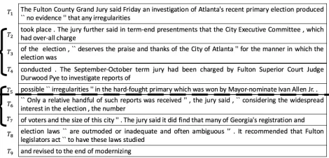
TextTiling is a query-independent segmentation algorithm. It assumes that each document is composed of a linear se-quence of segments, each of which represents a coherent topic. TextTiling inputs a document and outputs a list of top-ical segments. Figure 2 shows an excerpt from a long doc-ument that is used as a walking example to illustrate the al-gorithm. The algorithm takes three steps: Token Sequence Generation, Similarity Computation, and Boundary Deter-mination.
1. Token Sequence Generation: We start with splitting a
document into token sequences. Atoken sequenceis like a pseudo-sentence, which contains a fixed number of words. After removing the stopwords, everyα(set to 20 as recommended by Hearst) words are grouped into a to-ken sequence.1 These non-overlapping token sequences
1
Figure 2: TextTiling (α= 20, β = 3, stopwords are kept to preserve readability).
are the basic units to form a segment. In Figure 2, each line is a token sequence, denoted asTi, withiindexes the sequences starting from 1.
2. Similarity Computation:Once obtaining the token
se-quences, the topical boundaries would be determined based on the similarity between the sequences as well as its contexts. The context for a token sequence is a sliding window of sizeβ.βis set to 6 as recommended by Hearst. The similarity for two neighboring sequences is calcu-lated over the two windows to which they each belong. Formally, given n token sequences, T1, T2..., Ti, ..., Tn, the similarity between Ti and Ti+1 is calculated as the
cosine similarity of term counts (tf) in the two windows [Ti−β+1, ..., Ti]and[Ti+1, ..., Ti+β]:
sim(i, i+ 1) =
∑
wjtf(wj, i−β+ 1, i)·tf(wj, i+ 1, i+β) ||tf(w∗, i−β+ 1, i)|| · ||tf(w∗, i+ 1, i+β)||
(1)
wherewj is thejth word in the vocabulary,tf(wj, i−
β+ 1, i)
is the term frequency ofwjin a window holding sequencesTi−β+1, ..., Ti, andtf
(
wj, i+ 1, i+β
)
is the term frequency ofwjin a window holdingTi+1, ..., Ti+β, ||tf(w∗, i−β+ 1, i)||=sqrt(∑wjtf(wj, i−β+ 1, i)
2),
||tf(w∗, i+ 1, i+β)||=sqrt(∑wjtf(wj, i+ 1, i+β)2).
Figure 2 illustrates an example to computesim(4,5)with
β= 3. The similarity between token sequencesT4andT5
is computed based on the window upto and includingT4,
i.e.[T2, T3, T4], and the window afterT4, i.e.[T5, T6, T7].
We obtain a similarity score for every neighboring pairs of token sequences.
3. Boundary Determination:The previous steps result in
a series of similarity scores, each of which is created for a pair of token sequences. When plotting the similar-ity scores, we can observe “peaks” and “valleys” in this curve. When there is a dramatic drop in the curve, we say there is a possible topic change. A depth score is com-puted for each neighboring pairs of token sequences. It is defined as the sum of the absolute differences to its clos-est neighboring “peaks”. Thedepthscore betweenTiand
boundaries, rarely some token sequences are permitted to have sizes slightly different from 20.
Ti+1is
depth(i, i+ 1) =|sim(Lef tP eak(i, i+ 1)) −sim(i, i+ 1)|
+|sim(RightP eak(i, i+ 1)) −sim(i, i+ 1)|
(2)
where Lef tP eak computes the position of the closest “peak” on the left side and RightP eak computes that on the right side. Boundaries are discovered at positions where the depth score is greater thanµ−δ/2, whereµ
is the mean depth in the document andδ is the standard deviation. The threshold adjusts to different documents. In Figure 2, a boundary is found betweenT5andT6. Two
topical segmentsB1(containingT1, T2, ...) andB2
(con-tainingT6, T7, T8and the rest) are generated for the
doc-ument. When examining the actual content of these seg-ments, we find that the two segments represent distinct topics: one is the overview of an investigation and another is about the jury’s opinion.
TextTiling was a pioneering work in the 1990s for text segmentation. Unlike segmentation by a fixed passage length or by natural paragraphs, TextTiling’s segments are based on term distributions and are expected to be topic-coherent. More sophisticated text segmentation methods have been proposed since. Examples include probabilis-tic models that use language modeling and language cues (Beeferman, Berger, and Lafferty 1999), clustering-based al-gorithms (Kazantseva and Szpakowicz 2011), topic model-ing (Misra et al. 2009), and the recently proposed deep learn-ing methods (Badjatiya et al. 2018). Compared with Text-Tiling, most successor approaches still hold the assumption that topics are laid sequentially in a document. Without loss of generality, we use TextTiling for its simplicity and effec-tiveness and focus on how a segment-based visualization can aid neural information retrieval.
Standardizing Dimensions
Each segmentBiwould contain a different number of token sequences; and the total number of segments in a document would also vary from document to document. Note that this number is not only decided by the choices of token-sequence length (α) and window size (β) but also determined by the content of a document. In our experiments, there are docu-ments consisting only of a title, which yield only one seg-ment; whereas other longer documents split into hundreds of segments. As a result, for different query and document pairs, the dimensions of their TileBars visualizations vary. However, a neural network requires all its input vectors to be of equal size. We therefore need a mechanism to stan-dardize the TileBars visualizations.
Suppose the original dimension of an image is x×y, wherexis the query length andyis the number of segments. Our task is to resize all visualizations to a chosen dimension
nq×nb.
used in computer vision (Szeliski 2010). For queryq, itsith
wordwiis transformed into
wi′=
{
wi i≤x
⟨empty word⟩ x < i≤nq (3)
wherexis the length of original query andnqis the length of the transformed query and set to the maximum query length in the query collection.
Similarly to the query dimension, ify ≤nb, i.e. the orig-inal document is relatively short, then, zero padding is done and each segment is transformed by:
B′i=
{
Bi i≤y
⟨empty segment⟩ y < i≤nb (4)
whereBi′ is the segment after transformation andBi is the original segment.yis the original number of segments.
For documents with more thannbsegments, we ‘squeeze’ the content after (and including) thenbthsegment into the
nbthsegment, which makes the nbth segment the last in a document. This would preserve all the original content while only affect “resolution” of the last segment. Thus, ify > nb, i.e., the original document is relatively long, then
Bi′=
{
Bi i < nb
concatenate(Bnb, Bnb+1, ...By) i=nb (5)
After resizing, the visualization dimensions are fixed as
nq×nbfor all query-document pairs. From now on, we de-note query words aswand segments asBafter the standard-ization for the sake of notation simplicity.
Coloring
The original TileBars dyes the grids based only term fre-quency. The darker the color, the larger the intensity. In our work, we propose to incorporate multiple relevant features, similar to canonical colors in a color space, to “paint” the cells. Following the convention in multimedia research, we call each relevance feature a channel.
In theory, features indicating query-document relevance that are effective in existing learning-to-rank models can all be used here. However, to avoid interfering with the neural network’s ability to select the best feature combinations, we propose to only employ features that are independent of each other. It is similar to only use a few scalar valued colors as the canonical colors in a color space, and leave the feature aggregation to the network itself.
Three features are used in this work. They are all proven to be essential in ad-hoc retrieval. They are term frequency, inverse document frequency, and word similarity based on distributional hypothesis. The(i, j)thcell in the matching visualizationIfor querywand segmentBjis ‘painted’ by:
⎛
⎝
tf(wi, Bj)
idf(wi)×IBj(wi)
maxt∈Bje
−(vwi−vt)2
⎞
⎠ (6)
where wi is the ith query term, Bj is the jth text seg-ment in a docuseg-ment, tf(wi, Bj)is the term frequency of
wi in Bj, and idf(wi) is the inverse document frequency
of wi. IBj(wi) is an indicator function to show whether
wi is present in Bj. vt is the embedded word vector of word t, which comes from a pre-trained word2vec model (Mikolov et al. 2013). We use Gaussian kernels as suggested by (Xiong et al. 2017; Pang et al. 2016a). Themaxoperator is used to select the most similar word.
DeepTileBar: Deep Learning with TileBars
We propose a novel deep neural network, DeepTileBars, to evaluate document relevance. It consists of three layers of networks. It starts with detecting relevance signals with a layer of CNNs, followed by a layer of Long Short Term Memories (LSTMs) (Hochreiter and Schmidhuber 1997) to aggregate the signals. And then it decides the final relevance with a Multiple Layer Perceptron (MLP). Figure 4 illustrates the architecture of DeepTileBars. The input to the network is annq×nbinteraction matrix.Word-to-Segment Matching
Following TileBars, DeepTileBars builds an interaction ma-trix by comparing a word and a topical segment. Each seg-ment presumably corresponds to a topic. Per word informa-tion within the same segment is absorbed into a single cell and the word-level matching is no longer supported.
Using the proposed word-to-segment matching, we are able to produce relevance signals at the topic level and focus on the presence of query terms in consecutive topics. Match-ing queries to documents at the topic level, rather than at the word level, is perhaps easier to detect the stronger relevance signals with a bigger chunk of coherent text.
Our design is especially beneficial for proximity queries within a large window size. Most existing Neu-IR mod-els would be sufficient for proximity queries within a tight window, e.g. 2 or 3 words apart (Hui et al. 2017; Pang et al. 2016a). However, when the required window size is large, scanning a word-to-word matching with CNNs might miss the true relevant. A word-to-segment matching, in-stead, could resolve this issue by merging topically coherent words into a single segment and obtain a stronger relevance signal. In addition, as demonstrated in Figure 1, segment-based matching would eliminate high hits in spam passages thus avoid false positives.
Bagging with Different Kernel Sizes
TextTiling partitions a document into segments and the seg-ments are laid out sequentially without any further organiza-tion. However, topics in documents are often organized hier-archically. We can imagine that the segments form sections, and section form chapters, etc. If we could put several topi-cal segments together, they might actually form a super topic – a topic that is at a higher level. It would thus be desirable if the topics and super topics can be handled at different gran-ularities so that their hierarchical nature can be preserved.
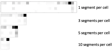
Figure 3: Word-to-segment matching at different granularity levels. Document enwp00-69-13554 for TREC 2011 Web Track query 116: California franchise tax board.
that each granularity level provides different relevance pat-terns for the same document. A relevant pattern can appear at any level. Looking at the relevance patterns at all levels would thus increase our chances of finding the true relevant. We thus propose to employ multiple CNNs (Krizhevsky, Sutskever, and Hinton 2012) with various kernel sizes to de-tect the relevance signals. Here we assume the kernel sizes vary from 1 tol, wherel is the maximum number of seg-ments the CNNs can handle. Practically, our model provides a hierarchical organization: token sequences are built from terms, segments (topics) are built from token sequences, and super topics are built by grouping adjacent topics with larger kernel sizes.
The Network
Figure 4 illustrates the network architecture. In the first CNN layer, there are l CNNs, [CN N1, CN N2, ..., CN Nk, ..., CN Nl]. Each CNN’s kernel size differs. For the kth CNN, its kernel size is
nq ×k. When each CNN scans through the input visual-ization, it produces a “tape”-like output. Askincreases, the CNNs are able to capture the relevance signals atkadjacent text segments. We call these k adjacent text segments ‘k-segment’. Thelnumber of CNNs produceloutputs. The output from the kth CNN denotes the relevance detected from all k-segments in the document. The shape of the
kth output is not a square, but a thin tape with dimension 1×(nb−k+ 1).
Note that Figure 3 is not the outputs of the CNNs. In-stead, it shows the relevance signals per query term when combining adjacent topical segments. The CNN outputs are the third column of thin-tapes in Figure 4.
The CNN layer is denoted asz0. The computation ofzk0
with kernel sizekis defined as
z0k=CN Nk(I), k= 1,2,3, ..., l (7)
More specifically,
z0k[i] = act
⎛
⎝
|channels|
∑
ch=1
nq−1
∑
u=0
k−1
∑
v=0
θk,ch0 [u, v]
∗I[u, i+v, ch] +b0k
⎞
⎠ (8)
Figure 4: DeepTileBars Architecture.
whereactis the ReLU activation function,chis the channel index,θis the kernel coefficient, andbis the bias.
At the second LTSM layer, in order to minimize the loss of information, we use the samelnumber of LSTMs to ac-cumulate the relevance signals. The output of thekthCNN is fed into thekthLSTM. An LSTM scans through its in-put step by step from the beginning to the end. The kth LSTM then outputs its evaluation of the entire document at the granularity ofk. For instances, the first LSTM,LST M1,
accumulates relevance signals from all the1-segments; the second LSTM, LST M2, accumulates those from all 2
-segments. Thus, the LSTMs layer is able to output multiple relevance estimations at different granularities.
When scanning at the tth timestep, where t =
1,2, ..., nb−k+ 1, thekthLSTM works as the following:
ftk =σ(Wfk[zk0[t], ht−1] +bkf)
ikt =σ(Wik[zk0[t], ht−1] +bki)
okt =σ(Wok[zk0[t], ht−1] +bko)
ckt =ftk∗ckt−1+ikt ∗tanh(Wck[zk0[t], hkt−1] +bkc)
hkt =okt ∗tanh(ckt)
(9)
whereσ()is the hard sigmoid activation function,ftk,ikt, and
ok
t are the values of the forget gate, input gate, and output gate.ck
tis the state.Wfk, W k
i, Wok, Wckandbkf, b k
i, bko, bkc are the weights and biases for the corresponding gates,hk
t is the output, and[]is the concatenation operator. The computation of the second layerz1is thus
z1k=LST Mk(zk0) =h k
nb−k+1, k= 1,2,3, ..., l (10)
At the third layer of MLP, all outputs of LTSMs are con-catenated together and fed into the layer to generate the final relevance decision. The computation of the third layersis
s=M LP([z1 1, ...zl1]).
To summarize, the overall architecture (see Figure 4) of DeepTileBars is:
zk0=CN Nk(I), k= 1,2,3, ..., l (11)
z1k=LST Mk(zk0), k= 1,2,3, ..., l (12)
We use a state-of-the-art Stochastic Gradient Descent (SGD) optimizer, Adam (Kingma and Ba 2015), to op-timize the network. We also adopt the L2 regulariza-tion (at the first layer) and early stopping to avoid over-fitting. The document ranking scores are obtained by a pairwise ranking loss function as in RankNet (Burges et al. 2005). It maximizes the difference between the rele-vant documents and the irrelerele-vant documents: J(Θ) =
∑
(q,d+,d−)−log 1
1+e−(s(d+,Θ)−s(d−,Θ)), where s is neural network output (Eq. 13),Θare the network parameters, and
q,d+, andd− are query, relevant document and irrelevant document, respectively.
Experiment
We evaluate DeepTileBars’ effectiveness on standard testbeds, including TREC Web Tracks and LETOR 4.0. We compare the performance of DeepTileBars with both tradi-tional IR approaches and the state-of-the-art Neu-IR models.
Dataset and Metrics
We conduct experiments on the TREC 2010-2012 Web Track Ad-hoc tasks (Clarke, Craswell, and Voorhees 2012).2 There are 50 queries each year. We combine the three years’ data as a single dataset because the annotated data from any single year is not enough to train a deep model. In total, there are 150 queries and 38,948 judged documents. Our experiment is conducted on ClueWeb09 Category B, which contains more than 50 million English webpages (231 Gi-gabytes in size).3We implement a 10-fold cross-validation for fair evaluation. The official metrics used in TREC 2010-2012 Web Track ad-hoc tasks include Expected Recipro-cal Rank (ERR)@20 (Chapelle et al. 2009), normalized Discounted Cumulative Gain (nDCG)@20 (J¨arvelin and Kek¨al¨ainen 2002) and Precision (P)@20. ERR and nDCG handle graded relevance judgments and Precision handles binary relevance judgements.
We also test our full model on the most recent MQ2008 dataset for LETOR 4.0. LETOR 4.0 is a common bench-mark used by Neu-IR models. LETOR MQ2008 contains 784 queries and 15,211 annotated documents. The official metrics used in LETOR includes nDCG and Precision at dif-ferent cutoff positions. We report results on queries that have at least one relevant documents in the judgment set.
Systems to Compare
• Traditional IR models:BM25(Robertson, Zaragoza, and others 2009) andLM(Zhai and Lafferty 2017). Both are highly effective IR models.
• TREC Best Runs: TREC Best is not a single system. In-stead, it is a combination of best systems per year per metric, including the best systems in 2010 (Elsayed et al. 2010; Dinc¸er, Kocabas, and Karaoglan 2010), 2011 (Boytsov and Belova 2011) and 2012 (Al-akashi and
2
TREC 2009 also had the Web Track. However, it used rele-vance scales and metrics quite different from the other years. For fairness and consistency, our experiments exclude year 2009.
3
http://lemurproject.org/clueweb09/.
Run err@20 ndcg@20 p@20
TREC-Best 0.188 0.236 0.382
BM25 0.102 0.137 0.253
LM 0.118 0.166 0.297
DRMM 0.127 0.184 0.346
MatchPyramid 0.113 0.125 0.228
DeepRank 0.127 0.134 0.224
HiNT 0.157 0.205 0.322
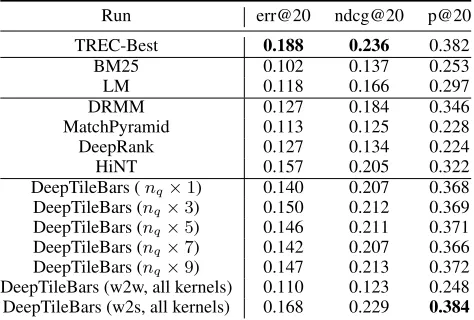
DeepTileBars (nq×1) 0.140 0.207 0.368 DeepTileBars (nq×3) 0.150 0.212 0.369 DeepTileBars (nq×5) 0.146 0.211 0.371 DeepTileBars (nq×7) 0.142 0.207 0.366 DeepTileBars (nq×9) 0.147 0.213 0.372 DeepTileBars (w2w, all kernels) 0.110 0.123 0.248 DeepTileBars (w2s, all kernels) 0.168 0.229 0.384
Table 1: TREC 2010-2012 Web Track Ad-hoc Tasks.
Inkpen 2012). We believe they represent the best perfor-mance of TREC submissions from 2010 to 2012.
• Neu-IR models: DRMM, MatchPyramid, DeepRank,
HiNT,DUET.4
• Variations of the proposed model:DeepTileBars (nq×x) that uses a CNN with a single kernel sizenq×x;
Deep-TileBars (w2w, all kernels), which uses all kernels with word-to-word matching; andDeepTileBars(w2s, all ker-nels), our full model, using word-to-segment matching and all kernels.
Parameter Settings
For the TextTiling algorithm, we set αto 20 and β to 6, as recommended by Hearst. For the query-document inter-action matrix, the parameters are slight differences between the two datasets. In TREC Web, nq = 5and In LETOR
nq = 9.nq is decided by the longest query after removing stopwords. For both datasets,nb= 30. This is because more than 90% documents in TREC Web and more than 80% doc-uments in LETOR contain no more than30segments.
For the DeepTileBars algorithm, we setl = 10for both datasets. In TREC Web Track dataset, the number of filters of CNN with same kernel size and the number of units in each LSTM are both set to3; while in LETOR, this number is set to 9. The MLP contains two hidden layers, with32and 16units for TREC Web, and128and16units for LETOR.
On the TREC Web dataset, we re-implement DRMM, MatchPyramid, DeepRank, HiNT by following the config-urations in their original papers. On LETOR, we include the reported results in their publications in Table 2 without re-peating the experiments.
Results
Tables 1 and 2 report our experimental results for the TREC Web Tracks and the LETOR MQ2008 datasets. Official met-rics are reported here.
4
Run p@5 p@10 ndcg@5 ndcg@10 Reported by BM25 0.337 0.245 0.461 0.220 (Qin and Liu 2013)
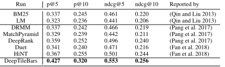
LM 0.323 0.236 0.441 0.206 (Qin and Liu 2013) DRMM 0.337 0.242 0.466 0.219 (Pang et al. 2017) MatchPyramid 0.329 0.239 0.442 0.211 (Pang et al. 2017) DeepRank 0.359 0.252 0.496 0.240 (Pang et al. 2017) Duet 0.341 0.240 0.471 0.216 (Fan et al. 2018) HiNT 0.367 0.255 0.501 0.244 (Fan et al. 2018) DeepTileBars 0.427 0.320 0.553 0.256
Table 2: LETOR-MQ2008.
It can be found that in the TREC Web Track dataset, DRMM, HiNT and our model DeepTileBars outperform tra-ditional IR approaches. While other neural IR approaches, MatchPyramid, DeepRank do not perform as well on certain metrics. On the LETOR dataset, all the Neu-IR approaches achieve better performance than traditional methods. It indi-cates that properly designed deep neural networks could im-prove upon traditional approaches. We also notice that with different network architectures and different input formula-tions, the Neu-IR models achieve varied gains. It would be worthwhile exploring which architecture is a better fit for ad-hoc retrieval.
It is exciting to see that our model, DeepTileBars, outper-forms other state-of-the-art neural IR systems in TREC Web Tracks and MQ2008. We think the gains come from the top-ical segmentation of the texts and the bagging of multiple CNNs with different kernel sizes. Word-to-segment match-ing provides relevance signals at the topic level. CNNs with different kernel sizes allow to evaluate document relevance at all granularities.
To investigate how DeepTileBars works internally, we ex-periment with a few variants of DeepTileBars with only one kernel. It can be found that adjusting the kernel size can only bring marginal improvement while the combination of all kernels boosts the retrieval performance.
When changing to-segment matching back to word-to-word matching, we observe a huge performance decrease. This confirms our claim that word-to-word matching is less desirable than word-to-segment matching in terms of finding relevance patterns.
However, we are still left behind by the TREC Best runs in some metrics. Some TREC Best runs used sophisticated term weighting methods without any deep learning (Dinc¸er, Kocabas, and Karaoglan 2010; Al-akashi and Inkpen 2012). Others used shallow neural networks or linear regression but with abundant feature engineering (Elsayed et al. 2010; Boytsov and Belova 2011). We look forward to the day when Neu-IR could catch up with the TREC best systems.
Related Work
There are only a few pieces of research that share similar intention with ours, i.e. visualizing the relevance signals in a document for deep learning. Works that are the closest to ours are MatchPyramid, HiNT, and ViP (Fan et al. 2017).
MatchPyramid was proposed for text matching tasks, in-cluding paraphrase identification and paper citation match-ing. By plotting the similarity between two sentences in an
n×mmatrix, wherenandmare the lengths of two sen-tences respectively, deep neural networks were used to find
the matching patterns between sentences with this image-like visualization. In MatchPyramid, the matching is done at the word level and experiments show it is less effective.
The more recent Neu-IR model, HiNT, adopted a simi-lar idea to ours to perform passage-level retrieval. One ma-jor difference between HiNT and DeepTileBars is how they split the documents. HiNT splits documents by fixed sized passages whereas DeepTileBars splits them based on topic changes. The passages in HiNT are in fact more similar to our token sequences, which do not represent topical struc-ture. As a result, the highest semantic level that HiNT is able to examine is similar to our segments. Levels higher than segments are not modeled in HiNT. In this sense, HiNT is not a true hierarchical Neu-IR model; instead, it is a segment-level only model. Meanwhile, although HiNT used a much more complex neural method, with a light-weighted architecture, DeepTileBars achieves better retrieval effec-tiveness in our experiments.
ViP also proposed to take advantage of visual features in a document. Instead of using the interaction matrix as the input image, ViP directly used a webpage’s snapshot as so. ViP’s experiments showed that even query-independent vi-sual features would be able to improve the retrieval effec-tiveness. ViP’s semantic units, such as the webpage sections and multimedia components, are similar to our hierarchical topics higher than the segments. In this sense, they are the most similar work to ours. However, we did not compare to their work in this paper due to our focus on texts.
Research from the field of Natural Language Processing has adopted similar designs of using multiple CNN kernel sizes. For example, (Kim 2014) used that for sentence clas-sification. Their input was ad×minteraction matrix, where
dwas the dimension of the term vectors andmwas the num-ber of words in a sentence. They encoded a sentence using multiple CNNs with kernel sizes d×n, where nwas the size of ann-gram and obviously could vary. While our use of multiple kernel sizes is driven by the attempt to fuse rel-evance signals at multiple topical granularities, their mod-ern way of representingn-grams (with different n) yielded a similar design to ours.
Conclusion
Acknowledgement
This research was supported by NSF CAREER Award IIS-145374. Any opinions, findings, conclusions, or recommen-dations expressed in this paper are of the authors, and do not necessarily reflect those of the sponsor.
References
Al-akashi, F. H., and Inkpen, D. 2012. Query-structure based web page indexing. InTREC’12.
Badjatiya, P.; Kurisinkel, L. J.; Gupta, M.; and Varma, V. 2018. Attention-based neural text segmentation. InECIR’18.
Beeferman, D.; Berger, A.; and Lafferty, J. 1999. Statistical models for text segmentation.Machine learning34(1-3):177–210. Boytsov, L., and Belova, A. 2011. Evaluating learning-to-rank methods in the web track adhoc task. InTREC’11.
Burges, C.; Shaked, T.; Renshaw, E.; Lazier, A.; Deeds, M.; Hamil-ton, N.; and Hullender, G. 2005. Learning to rank using gradient descent. InICML’05.
Byrd, D. 1999. A scrollbar-based visualization for document nav-igation. InDL’99.
Chapelle, O.; Metlzer, D.; Zhang, Y.; and Grinspan, P. 2009. Ex-pected reciprocal rank for graded relevance. InCIKM’09. Clarke, C. L. A.; Craswell, N.; and Voorhees, E. M. 2012. Overview of the trec 2012 web track. InTREC’12.
Dinc¸er, B. T.; Kocabas, I.; and Karaoglan, B. 2010. Irra at trec 2010: Index term weighting by divergence from independence model. InTREC’10.
Elsayed, T.; Asadi, N.; Wang, L.; Lin, J. J.; and Metzler, D. 2010. Umd and usc/isi: Trec 2010 web track experiments with ivory. In TREC’10.
Fan, Y.; Guo, J.; Lan, Y.; Xu, J.; Pang, L.; and Cheng, X. 2017. Learning visual features from snapshots for web search. In CIKM’17.
Fan, Y.; Guo, J.; Lan, Y.; Xu, J.; Zhai, C.; and Cheng, X. 2018. Modeling diverse relevance patterns in ad-hoc retrieval. In SI-GIR’18.
Guo, J.; Fan, Y.; Ai, Q.; and Croft, W. B. 2016. A deep relevance matching model for ad-hoc retrieval. InCIKM’16.
Hearst, M. A. 1994. Multi-paragraph segmentation expository text. InACL’94.
Hearst, M. A. 1995. Tilebars: visualization of term distribution information in full text information access. InCHI’95.
Hearst, M. 2009. Search user interfaces. Cambridge University Press.
Hochreiter, S., and Schmidhuber, J. 1997. Long short-term mem-ory.Neural computation9(8):1735–1780.
Hornbæk, K., and Frøkjær, E. 2001. Reading of electronic docu-ments: the usability of linear, fisheye, and overview+ detail inter-faces. InCHI’01.
Huang, P.-S.; He, X.; Gao, J.; Deng, L.; Acero, A.; and Heck, L. 2013. Learning deep structured semantic models for web search using clickthrough data. InCIKM’13.
Hui, K.; Yates, A.; Berberich, K.; and de Melo, G. 2017. Pacrr: A position-aware neural ir model for relevance matching. In EMNLP’17.
J¨arvelin, K., and Kek¨al¨ainen, J. 2002. Cumulated gain-based eval-uation of ir techniques.ACM Transactions on Information Systems (TOIS)20(4):422–446.
Kazantseva, A., and Szpakowicz, S. 2011. Linear text segmentation using affinity propagation. InEMNLP’11.
Kim, Y. 2014. Convolutional neural networks for sentence classi-fication. InEMNLP’14.
Kingma, D. P., and Ba, J. 2015. Adam: A method for stochastic optimization.ICLR’15.
Krizhevsky, A.; Sutskever, I.; and Hinton, G. E. 2012. Ima-genet classification with deep convolutional neural networks. In NIPS’12.
Liu, T.-Y., et al. 2009. Learning to rank for information retrieval. Foundations and Trends⃝R in Information Retrieval3(3):225–331.
Mann, W. C., and Thompson, S. A. 1988. Rhetorical structure the-ory: Toward a functional theory of text organization.Text8(3):243– 281.
Mikolov, T.; Sutskever, I.; Chen, K.; Corrado, G. S.; and Dean, J. 2013. Distributed representations of words and phrases and their compositionality. InNIPS’13.
Misra, H.; Yvon, F.; Jose, J. M.; and Cappe, O. 2009. Text seg-mentation via topic modeling: an analytical study. InCIKM’09. Mitra, B.; Diaz, F.; and Craswell, N. 2017. Learning to match using local and distributed representations of text for web search. InWWW’17.
Nguyen, G.-H.; Soulier, L.; Tamine, L.; and Bricon-Souf, N. 2017. Dsrim: A deep neural information retrieval model enhanced by a knowledge resource driven representation of documents. In IC-TIR’17.
Pang, L.; Lan, Y.; Guo, J.; Xu, J.; and Cheng, X. 2016a. A study of matchpyramid models on ad-hoc retrieval. Neu-IR’16 SIGIR Workshop on Neural Information Retrieval.
Pang, L.; Lan, Y.; Guo, J.; Xu, J.; Wan, S.; and Cheng, X. 2016b. Text matching as image recognition. InAAAI’16.
Pang, L.; Lan, Y.; Guo, J.; Xu, J.; Xu, J.; and Cheng, X. 2017. Deeprank: A new deep architecture for relevance ranking in infor-mation retrieval. InCIKM’17.
Qin, T., and Liu, T. 2013. Introducing LETOR 4.0 datasets.CoRR abs/1306.2597.
Robertson, S.; Zaragoza, H.; et al. 2009. The probabilistic rele-vance framework: Bm25 and beyond. Foundations and Trends⃝R
in Information Retrieval3(4):333–389.
Shen, Y.; He, X.; Gao, J.; Deng, L.; and Mesnil, G. 2014. Learning semantic representations using convolutional neural networks for web search. InWWW’14.
Skorochod’ko, E. F. 1971. Adaptive method of automatic abstract-ing and indexabstract-ing. In Freiman, C. V., ed.,Proceedings of the IFIP Congress 71, volume 2, 1179–1182.
Szeliski, R. 2010. Computer vision: algorithms and applications. Springer Science & Business Media.