R E S E A R C H
Open Access
Faster algorithms for RNA-folding using the
Four-Russians method
Balaji Venkatachalam
*, Dan Gusfield and Yelena Frid
Abstract
Background: The secondary structure that maximizes the number of non-crossing matchings between complimentary bases of an RNA sequence of lengthncan be computed inO(n3)time using Nussinov’s dynamic programming algorithm. The Four-Russians method is a technique that reduces the running time for certain dynamic programming algorithms by a multiplicative factor after a preprocessing step where solutions to all smaller
subproblems of a fixed size are exhaustively enumerated and solved. Frid and Gusfield designed anO(logn3n)algorithm for RNA folding using the Four-Russians technique. In their algorithm the preprocessing is interleaved with the algorithm computation.
Theoretical results: We simplify the algorithm and the analysis by doing the preprocessing once prior to the algorithm computation. We call this thetwo-vectormethod. We also show variants where instead of exhaustive preprocessing, we only solve the subproblems encountered in the main algorithm once and memoize the results. We give a simple proof of correctness and explore the practical advantages over the earlier method.
The Nussinov algorithm admits anO(n2)time parallel algorithm. We show a parallel algorithm using the two-vector idea that improves the time bound toO(logn2n).
Practical results: We have implemented the parallel algorithm on graphics processing units using the CUDA platform. We discuss the organization of the data structures to exploit coalesced memory access for fast running times. The ideas to organize the data structures also help in improving the running time of the serial algorithms. For sequences of length up to 6000 bases the parallel algorithm takes only about 2.5 seconds and the two-vector serial method takes about 57 seconds on a desktop and 15 seconds on a server. Among the serial algorithms, the two-vector and memoized versions are faster than the Frid-Gusfield algorithm by a factor of 3, and are faster than Nussinov by up to a factor of 20. The source-code for the algorithms is available athttp://github.com/
ijalabv/FourRussiansRNAFolding.
Keywords: RNA-folding, Four-Russians, CUDA, Algorithms, Parallel algorithm, GPU
Background
Computational approaches to find the secondary struc-ture of RNA molecules are used extensively in bioinfor-matics applications.
The classic dynamic programming (DP) algorithm pro-posed in the 1970s has been central to most structure prediction algorithms. While the objective of the original algorithm was to maximize the number of non-crossing
*Correspondence: [email protected]
Department of Computer Science, University of California, Davis, 1 Shields Ave, Davis, CA, USA
pairings between complementary bases, the dynamic pro-gramming approach has been used for other models and approaches, including minimizing the free energy of a structure. The DP algorithm runs in cubic time and there have been many attempts at improving its running time [1,2]. Here, we use the Four-Russians method for speeding up the computation.
The Four-Russians method, named after Aralazarov et al. [3], is a method to speed up certain dynamic programming algorithms. In a typical Four-Russians algo-rithm there is a preprocessing step that exhaustively enu-merates and solves a set of subproblems and the results are tabled. In the main DP algorithm, instead of filling out
or inspecting individual cells, the algorithm takes longer strides in the table. The computation for multiple cells is solved in constant time by utilizing the preprocessed solu-tions to the subproblems. The longer strides to fill the table reduce the runtime by a multiplicative factor. The size of the subproblems is chosen in a way that does not make the preprocessing too expensive.
Frid and Gusfield [4] showed the application of the Four-Russians approach for RNA folding. In their algorithm, the preprocessing is interleaved with the algorithm com-putation. They fill out a part of the DP table and use these entries to complete a part of the preprocessing. The preprocessed entries are used later in the computation.
We show a simpler algorithm, where, all the preprocess-ing is completed before the start of the main algorithm. This simplifies the correctness proof and the runtime analysis. This approach helps in obtaining anO(n3/logn) time parallel algorithm, which is a lognfactor improve-ment over previously-known parallel algorithms. Zakov and Frid (personal communication) had also observed that the algorithm in [4] could be modified to do the preprocessing once at the start of the algorithm. It is essentially the idea described here.
In this paper we explore the implications of the one-pass preprocessing idea. This description of the algorithm leads naturally to two other variants. We empirically eval-uate these variants and also the implementation of the parallel algorithm.
The parallel architecture of general-purpose graphical processing units (GPUs) have been exploited for many real-world application in addition to applications in gam-ing and visualization problems.
GPUs have also been used to speed up RNA folding algorithms [5-7]. Here we show how the Four-Russians method allows an organization of the data structures for fast memory accesses. We also describe the organization of the parallel hierarchy to exploit the inherent parallelism of the solution.
In the rest of the section, we describe the problem in relation to the other problems in RNA folding. To keep the paper self-contained, we will first describe the two-vector algorithm, our application of the Four-Russians method to the RNA folding problem. We will use that description to describe the original Four-Russians method for RNA folding by Frid and Gusfield [4]. This discus-sion leads to two other variants where the preprocessing is done on demand, instead of the exhaustive prepro-cessing in the two-vector method and the Frid-Gusfield algorithm. In Section ‘AnO(logn2n)parallel algorithm’ we discuss theO(n2/logn) parallel algorithm. We will then describe the implementation of a parallel algorithm using CUDA. The final sections have discussion on empirical observations and conclusions.
Related work
The O(n3) dynamic programming algorithm due to Nussinov et al. [8,9] maximizes the number of non-crossing matching complimentary bases. There have been many methods since Zuker and Stiegler [10] that infer the folding using thermodynamic parameters [11,12] which are more realistic than maximizing the number of base pairs. These methods have been implemented in many packages including UNAFold [13], Mfold [14], Vienna RNA Package [15], RNAstructure [16].
Probabilistic methods include stochastic context-free grammars [17,18], the maximum expected accuracy (MEA) method, where secondary structures are com-posed of pairs that have a maximal sum of pairing prob-abilities, e.g., MaxExpect [19], Pfold [20], CONTRAfold [21] which maximize the posterior probabilities of base pairs; and Sfold [22], CentroidFold [23] that maximize the centroid estimator. There are also other methods that use a combination of thermodynamic and statistical parame-ters [24] and methods that use training sets of known folds to determine their parameters, e.g., CONTRAfold [21], Simfold [25] and ContextFold [26].
In addition to the Four-Russians method, other methods to improve the running time include Valiant’s max-plus matrix multiplication by Akutsu [1] and Zakov et al. [2]; and sparsification, where the branch points are pruned to get an improved time bound [27,28].
CUDA, the programming platform for GPGPUs, has been used to solve many bioinformatics problems. Chang, Kimmer and Ouyang [5] and Stojanovski, Gjorgjevikj and Madjarov [7] show an implementation of the Nussinov algorithm on CUDA. Rizk et al. [6] describe the imple-mentation for Zuker and Stiegler method involving energy parameters. These methods are discussed later in the parallel implementation section.
The Nussinov algorithm
In this paper, we consider the basic RNA folding problem of maximizing the number of non-crossing complimen-tary base pair matchings. Complimencomplimen-tary bases can be paired, i.e.,AwithUandCwithG. A set of disjoint pairs is a matching. The pairs in a matching must not cross, i.e., if bases in positionsiandjare paired and if baseskandlare paired, then either they are nested, i.e.,i < k < l < jor they are non-intersecting, i.e.,i < j< k < l. The objec-tive is to maximize the number of pairings under these constraints.
D(i,j)=max
b(S(i),S(j))+D(i+1,j−1)
maxi+1≤k≤jD(i,k−1)+D(k,j) (1)
whereb(., .) = 1 for complimentary bases and 0 other-wise. The DP table is the upper triangular part of then×n matrix. The optimal solution is given byD(1,n). The table can be filled column-wise from the first column till the nth. There are other ways of filling the table too, e.g., along the diagonals — the(i,i)-diagonal first,(i,i+1)-diagonal next and so on, until the last diagonal with one entry, D(1,n). To allow for traceback we need to store the bases that are paired to get the maximum value. Let D∗(i,j) denote the corresponding indices. These are obtained by substituting arg max in place of max in the above recurrence and can be computed along with the max value.
The first part of the recurrence can be solved in constant time. The second part is more expensive, incurring(n) look ups and maximum computations. There are O(n2) entries in the DP table and each cell can be computed in O(n)time, giving anO(n3)time algorithm.
The Four-Russians algorithms
In this section we discuss three variants of the Four-Russians algorithm. We will first describe thetwo-vector approach. Since it is simpler than the other methods we will use the description to discuss two other variants.
Two-vector algorithm
To apply the Four-Russians technique we start with the following observation:
Lemma 3.1. The values along a column from bottom to top and along a row from left to right are monotonically non-decreasing. Consecutive cells differ at most by 1.
Proof.Consider the values of neighboring cells (i,j) and(i+1,j). D(i,j) represents the solution of a longer sequence than D(i + 1,j). Therefore the former value should be at least as large as the latter. SupposeD(i,j) dif-fered from D(i +1,j) by more than one. Then we can remove any matching for i. This has at most one fewer base pair matching and is a valid solution for the subse-quence(i+1,j)with a larger value than its current value, contradicting the optimality ofD(i+1,j). An analogous argument holds along the rows.
Once the cellsD(i,l),D(i,l+1),. . .,D(i,l+q−1)are computed, for somel ∈ {i,. . .,j−q}, they can be rep-resented byD(i,l)+V0, D(i,l)+V1,. . ., D(i,l)+Vq−1,
whereVp=D(i,l+p)−D(i,l), forp∈ {0,. . .,q−1}. Let us define,v0=0 andvp=Vp−Vp−1, forp∈ {1,. . .,q−1}. From lemma 3.1, vp ∈ {0, 1}, for all p ∈[0,q− 1]. Let
vdenote the binary vectorv0,v1,. . .,vq−1 of differences and letVdenote the vector of running totalsV0,V1,. . ., Vq−1.
Since thevp’s are defined from Vp’s, the inverse func-tion is well defined:Vp = pk=0vk. ThusD(i,l)together with the vector v represents q consecutive cells of the table.
Similarly, since the values are non-increasing down a column,D(i+l+1,j),. . .,D(i+l+q,j)be represented by the pairD(i+l+1,j),v¯, wherev¯∈ {0,−1}q. The corre-sponding vector of cumulative sums is denotedV¯. We call vthehorizontal difference vectoror thehorizontal vector and we callv¯thevertical difference vectoror thecolumn vector.
Considerqconsecutive cells froml+1 tol+qused in computingD(i,j):
D(i,j) ← max
l+1≤k≤l+q D(i,k−1)+D(k,j) (2)
← max
0≤k≤q−1 D(i,l)+Vk+D(i+l+1,j)+ ¯Vk
← D(i,l)+D(i+l+1,j)+ max
0≤k≤q−1 Vk+ ¯Vk (3)
As before, we use arg max in place of max to obtain D∗(i,j), which facilitates the traceback.
As noted above the second line of the recurrence (1), looping over elements, is more expensive part of the com-putation and we will use (3) instead of (2) to compute the Dand D∗ values in the Four-Russians method. That is, we will use (3) over groups ofqcells each instead of one loop of (1). Since theV vectors are in bijection with thev vectors, we will usevin the computation. Letvandv¯be the corresponding vectors in (3). The following algorithm evaluates the max computation.
Input: horizontal difference vectorvand vertical differ-ence vectorv¯
1: max-val←0 andmax-index←0 2: sum1←0 andsum2←0
3: fork=0 toq−1do 4: sum1←sum1+vi 5: sum2←sum2+ ¯vi
6: ifsum1+sum2>max-valthen 7: max-val←sum1+sum2 8: max-index←k
9: end if 10: end for
Using this instead of (2) is not advantageous in itself. How-ever, if this algorithm is given as a black box,D(i,j)can be computed in constant time by invoking the black box once. To exploit this fact, we will preprocess this compu-tation over all possible vandv¯ vectors and tabulate the results inR. TableRis indexed by a pair of numbers in the range [2q] to represent the two vectors(v,v¯). The table lookup is a constant time operation as it fetches the max and arg max values. We will show later that this exhaustive enumeration is not too expensive.
In the Nussinov algorithm described in the previous section, the recurrence overqcells is evaluated using (2) and it takesO(q)time. In the Four-Russians method, using the preprocessing step, the max computation is available through a table lookup and the recurrence forqterms can be completed in constant time. This reduction in the com-putation time is the reason for the speedup by a factor ofq. The two-vector method modifies the Nussinov algo-rithm as follows. All the rows and columns of the table are grouped into groups ofq cells each. The recurrence over theseqcells is computed in constant time using the preprocessing table. The recurrence involvesD(i,k−1)+
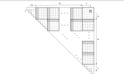
D(k,j), i.e., the value in the (k − 1)st column is used with thekthrow. Therefore the row and column group-ings differ by one. That is, the columns are grouped (0, 1,. . .,q−1), (q,q+1,. . ., 2q−1) etc. The rows are grouped(1, 2,. . .,q),(q+1,q+2,. . ., 2q)etc. This ensures that the row and column groups are well characterized. That is, to fill the cell(i,j), thekthgroup along rowineeds to be combined with thekthgroup below(i,j)in columnj. The cells of the table are filled in the same order as before. When the last cell of a row- or a column- group is evaluated the corresponding row and column vectors are computed and stored. To fill cell(i,j), we retrieve the first element and the horizontal vector of the group from rowi and the first element and the column vector from the cor-responding group in columnj. The recurrence is solved using (3) by a table lookup. The final value forD(i,j)is the maximum value over all the groups. There might be resid-ual elements in the row that do not fall in these groups. There are at most 2q such elements. These are solved separately using Nussinov’s method. Algorithm 1 has the algorithm listing and Figure 1 describes the algorithm pictorially.
Algorithm 1Procedure for the two-vector Four-Russians speedup. The DP table is filled column-wise. 1: R←preprocess all pairs of vectors of lengthq
2: forj=1 ton do 3: D(j,j)←0 4: D(j+1,j)←0
5: fori=j−1 down to 1 do
6: D(i,j)←b(S[i] ,S[j])+D(i+1,j−1) 7: Let(i,i)be in theIthgroup in rowi.
8: Let(i,j)be in theJthgroup horizontally in theithrow andJthgroup vertically in thejthcolumn. 9: LetiIbe the right-most entry of groupIandjJbe the left-most entry in groupJ
10: fork=i+1 toiIdo // For all cells in the first group 11: D(i,j)←max(D(i,j),D(i,k−1)+D(k,j))
12: end for
13: fork=jJ tojdo // For all cells in the last group 14: D(i,j)←max(D(i,j),D(i,k−1)+D(k,j)) 15: end for
16: forK =1 toJ−Ido // For all groups in between
17: Letlbe the left-most cell in theKthgroup to the right ofIandtbe the top-most cell in theKthgroup below J.
18: Letvi,K andv¯K,jbe the corresponding horizontal and vertical difference vectors. 19: D(i,j)←max(D(i,j),D(i,l)+D(t,j)+R(vi,K,v¯K,j))
20: end for
21: ifi modq=1then // compute the vertical difference vector 22: compute and store thevvectori/qthgroup for columnj
23: end if
24: ifj modq=q−1then // compute the horizontal difference vector 25: compute and store thev¯vector(j−1)/qthgroup for rowi
Figure 1A diagrammatic representation of the two-vector method.The row and column blocks are matched as labelled. The gray boxes and the gray dashes show the initial value and difference vectors. The group of cells inbcorrespond to the Four-Russians loop in lines 16–20 of Algorithm 1; the cells inaare used in the loop in lines 10–12 and the cells incform the loop in lines 13–15.
Runtime analysis
In the precomputation phase, there are 2q q-length vec-tors and 22qpairs of vectors. The precomputation takes O(q)time per vector pair. Thus the total time for precom-putation isO(q22q).
The main algorithm: There areO(n2) cells and to fill each cell it takesO(n/q+q)time. That is, it takesO(n/q) time to look up the initial value and the difference vec-tor and theRtable lookups for the theO(n/q)groups. It takesO(q) time for the residual elements. Thus it takes O(n2×(n/q+q))time to fill the table. Every cell is invol-ved in at most two vector computations, where the dif-ference to its neighbor is computed once for the row and for the column vector. This takes an amortizedO(n2)time which is dominated by the rest of the algorithm.
Whenq=logn, the total time for the entire algorithm is O(logn22 logn+n2+n2×(lognn+logn))=O(n2logn+ n3/logn)=O(n3/logn).
FG algorithm
Frid and Gusfield [4] first showed how the Four-Russians approach could be applied to the RNA-folding problem. We will call their algorithm theFGalgorithm.FGand two-vectoralgorithms are variants of the same idea. We will
highlight the differences in preprocessing and the maxi-mum value computation by the Four-Russians technique. In particular, we will show the maximum computation in step 19 of Algorithm 1.
After computing theq-contiguous cells of a group in a row, the value in the initial cellD(i,p)and the horizontal difference vectorvpare known. They run the preprocess-ing algorithm in page 3 for this fixedvp vector together with all possible vertical difference vectors. They add the value of D(i,p) to the maximum and table the result. This preprocessing step is computed for every block of every row. The preprocessing tableRis indexed by row number, group number and a vector (which is a poten-tial column vector). The horizontal vectors need not be stored.
Notice the difference between the two-vector and the FG variants. In two-vector algorithm the preprocessing for vector pairs is computed once for each distinct pair of vectors. Whereas, in FG the preprocessing step is run once for each group of each row, even if the vector pair was seen earlier. This is because the table contains the result of addition of the initial cell of the groupD(i,p).
vector in the corresponding block is retrieved from the table and the result is added toD(q,j).
The preprocessing is for horizontal vectors seen in the table. Since the horizontal vectors are not known before-hand, the precomputation cannot be done prior to the main algorithm. Instead, it is interleaved with the compu-tation of the table. They fill part of the DP table and use the vectors to complete some preprocessing, which in turn is used fill another part of the table and so on.
Since the preprocessing is done for every group of every row, the same horizontal vector can be seen multiple times in the table. This leads to duplicated work and slower running time than the two-vector algorithm.
The running time for the FG method isO(logn3
bn), where 2<b<nandbq=n.
Two variants that memoize
The two-vector method computes the preprocessing over all possible vector pairs. While the computation is for done exactly once for the unique vector pairs, some of these vector pairs might not be seen in the table. In the FG method, the precomputation step is for only the horizon-tal vectors that are seen in the table. However, for some vectors, the computation is duplicated. Stated this way, a hybrid approach suggests itself.
In our next variants, we memoize the results for a pair of vectors. Like the two-vector approach, the preprocess-ing is done only once for a vector pair and like the FG algorithm, it is only for the vectors seen in the table and the preprocessing is interleaved with the main algorithm. Since the preprocessing table is indexed by two vectors, unlike the FG algorithm, the results are computed only once for every vector seen.
In the partially memoized version, upon completion of elements of a group, if a new horizontal vector is seen, we pair it with all possible 2qcolumn vectors and the results are tabled. In the completely memoized version, the result for a pair of horizontal and vertical vectors are computed the first time the pair is observed and the result is stored in the table. The computed values for retrieved from the table when they are seen again. The rest of the algorithm is identical to the two-vector method.
All these variants takeO(n3/logn)time but the memo-ized versions potentially store fewer vectors than the two vector method and will have a similar worst-case run-time in practice as the two-vector method. But, as argued before, the FG method does duplicated work and will be slower in practice.
AnO(logn2n)parallel algorithm
The Nussinov DP algorithm can be parallelized with n processes to get an O(n2) parallel algorithm on a
concurrent-read concurrent-write parallel random access memory (CRCW PRAM) machine . In the parallel algo-rithm, we fill the table diagonal by diagonal. We use n processes and assign one parallel process to each column. In theithiteration, thepthprocess computes the value for the(p−i)thdiagonal entry. That is, in the first iteration, the bottom-most cell in each column, i.e., the entries in the main diagonal are solved and in successive iterations, the diagonals above are solved. To compute the value for cell(i,j), the entries in the row to its left and in the column below (i,j) are needed. The entries in the same column are computed in earlier iterations. Similarly, the entries on the left are solved by other processes in earlier itera-tions. Since these values are computed in earlier iterations, each diagonal cell can be filled independent of the other processes.
More formally, we havej∈[n] parallel processes and the jth process computes the values of values along the col-umnj. All processes synchronize after filling an entry; this ensures that values needed to fill a cell are computed by the other processes.
The parallel algorithm for processjforj=1, 2,. . .,n:
1: D(j+1,j)←0,D(j,j)←0 2: fori=jdown to 1 do
3: D(i,j)←D(i+1,j−1)+b(S[i] ,S[j]) 4: fork=i+1 tojdo
5: D(i,j)←max{D(i,j),D(i,k−1)+D(k,j)} 6: end for
7: Synchronize with other processes 8: end for
A process has to compute the value forO(n)cells and for each cell it needs to accessO(n)other cells. Thus the total computation takesO(n2)time withnprocesses.
We will describe the use the two-vector Four-Russians method to obtain an O(n2/logn) algorithm below. The preprocessing step that enumerates the solution for 2q × 2qdifference vectors is embarrassingly parallel and we do not discuss the parallel algorithm for it.
As before, we fill the table along the diagonals. We use nprocesses, one for each column. Each process solves the entries of the column from bottom to top. As in the serial algorithm, computing the maximum by looping over all the entries is the expensive part of the computation and will be optimized. Instead of looping over the individual entries (lines 4 – 6 in the parallel algorithm above), we use the Four-Russians technique to solveq cells in one step by looking up the table computed in the preprocessing step.
We modify the inner loop of the parallel algorithm as follows:
1: fork=0 toj/q −1do 2: k=i+k∗q
3: D(i,j) = max{D(i,j),D(i,k) + D(k + 1,j) + R[dH(i,k)] [dV(k+1,j)]}
4: end for
5: fork= j/q ×qtojdo
6: D(i,j)←max{D(i,j),D(i,k)+D(k+1,j)} 7: end for
8: Compute the horizontal and vertical differences and store them indH(i−q+1,j)anddV(i,j)respectively.
For each entry, the first loop takesO(n/q)time and the second loop takesO(q) time. Since all the processes are solving the kth diagonal in the kth iteration, all of them execute the same number of steps before synchronization. Note that we compute the horizontal and vertical differ-ences for every node, unlike in Algorithm 1 where they are computed everyqthcell, to ensure that every process performs the same number of steps and simplify the anal-ysis. The difference vectors can be computed inO(q)time. These can also be computed in constant time by shifting the previous difference vector and appending the new dif-ference. But we will not assume this simplification for the time bound computation.
Thus each entry can be computed inO(n/q+q)time. There areO(n)entries for each process, thus the total time taken for all processes to terminate isO(n2/q+nq). With q=lognas before, this gives anO(n2/logn)algorithm.
Parallel implementation
GPU architecture
Graphics processing units (GPUs) are specialized pro-cessors designed for computationally intensive real-time graphics rendering. In addition to manipulating graphics objects the parallel architecture can be exploited for other tasks where large amounts of data are to be processed in parallel. Compute Unified Device Architecture (CUDA) is the computing engine designed by NVIDIA for their GPUs. It allows the programmer to write highly parallel code and provides platform-specific optimizations.
In CUDA, a serial program on a “host” CPU launches parallel “kernels” on the “device” GPUs. Kernels specify the code to be executed by all the threads. Every thread executes the same code in a kernel but can be assigned a different part of the task based on their indices. This paradigm is called Single-Instruction Multiple-Thread (SIMT), which is similar to Single-Program Multiple Data (SPMD) where the threads are run almost in lockstep.
The programmer can group threads in a block, which in turn can be organized in agridhierarchy. The threads
in a block and blocks in a grid can be organized in one-, two- or three-dimensions. While the hierarchy is specified when launching a kernel, thread management is handled by the underlying system. The threads within a block use barrier synchronization. Different blocks communicate by atomic memory operations in global memory.
Memory hierarchy includes thread-specific local mem-ory, block-level shared memory for all threads in the block and global memory for the entire grid. The access times increases along the hierarchy from local to global memory. Kernels are very fast when threads run in lockstep. If certain threads take a conditional branch or are delayed by memory access then all the threads in the block are stalled. Since the access to global memory is slow (more clock cycles than local memory access), it is efficient for the threads within a block to access contiguous memory loca-tions. Then the hardwarecoalescesmemory accesses for all threads in a block into one request. More specifically, in our application, if a matrix is stored in row-major order and if the threads in a block access contiguous elements of a row, then the accesses can be coalesced. Whereas access-ing elements along a column is inefficient as distant mem-ory elements have to be fetched from different cache lines. Programs that observe the hardware specifications can exploit the optimizations in the system and are fast in practice. We designed the program that exploits the par-allel structure of the DP algorithm and the hardware features of the GPU.
Related work
As mentioned earlier, the cells of a diagonal are inde-pendent of one another and can be computed in parallel. In Stojanovski et al. [7], elements of the diagonal are assigned to a block of threads. This design does not handle memory coalescence for either row or column accesses. Chang et al. [5] allocate an n×n table and reflect the upper-triangular part of the matrix on the main diago-nal. Successive elements of a column are fetched from the row in the reflected part of the matrix. When threads of a block are assigned to elements of a diagonal, the successive column accesses for a thread are to consecutive mem-ory cells. However, this does not allow coalesced access for threads within a block. Rizk and Lavenier [6] show an implementation for RNA folding under energy mod-els. They show a tiling scheme where a group of cells are assigned to a block of threads to reuse the data values that are fetched from a column. In this paper, we show that storing the row and column vectors in different orders for two-vector method can further improve the efficiency.
Design of the Four-Russians CUDA program
The high-level idea
Like in the parallel algorithm described in Section ‘An
along the diagonals. However, for efficiency reasons, we cannot fill each diagonal in order. For example, by assign-ing different cells of a diagonal to a block of threads, each thread has to access a different row and different column. This design is not efficient as threads in a block try to access different locations of global memory which slows down the program. For the program to be efficient on the CUDA architecture, we exploit coalesced memory access for faster computation and ensure that individual threads are not stalled. We create a tiled table by groupingq×q cells into a tile and assign a block of threads to fill a tile. We will show that the tiles are independent and assign a grid of blocks to solve a diagonal of tiles in parallel. Thus the implementation can be thought of as a generalization of the Four-Russians algorithm on the tiled table. The details follow.
Data structures
Notice that cells D(i,j) and D(i− 1,j) both use values in columnjbelowD(i,j). Similarly,D(i,j+1)andD(i,j) refer to values in rowito the left of cell(i,j). By grouping these cells together and assigning this group to a block of threads the values along the rows and columns should be fetched once per block. We will groupq×qcells together and store the values from the rows and columns in shared memory. As noted earlier, for the four-Russians method, it is convenient to group the rowskq+1,. . .,(k+1)qand columnskq,. . .,(k+1)q−1, fork ∈ {0,. . .,n/q}. We now have atiled table, where each tile is a composite of q×q cells. The tiles along a diagonal can be computed independent of each other. Each tile is assigned to a block of threads and computed in parallel. After all the entries of the tile are computed, only the horizontal and vertical differences are stored. The horizontal and vertical differ-ence vectors are used by the Four-Russians technique for later computations.
To fill a tile, the horizontal differences of all the tiles to the left and vertical differences from the tiles underneath are accessed. By storing these difference vectors together the memory accesses can be coalesced. That is, we store the horizontal differences of the rows in a tile together. Similarly, the vertical differences of the tile are grouped together. However, the horizontal and vertical differences of the tiles are stored in different order. The horizontal differences are stored in row-major order and the verti-cal differences are stored in column-major order to exploit coalesced memory access.
When each thread retrieves one vector from a tile, the block of threads accesses contiguous memory locations and the memory accesses are coalesced. Successive itera-tions fetch the vectors from tiles along a row which are in contiguous memory locations. Similarly the vertical dif-ferences of a tile below are accessed in one coalesced memory access by the threads of the block.
Since we groupqelements together, at the last column of tiles might have fewer thanqelements and handling the corner cases at the GPU will involve extra checks which might slow the program down. We can avoid these by padding the sequence with extra characters. The modified string hasn = n+q−n modq characters. The final result is still stored in cellD(1,n).
Thread hierarchy
There are a few options for assigning threads to compute various cells in a tile. We can assignq2threads, one per cell, or assignqthreads, one per row or column. While it appears thatq2threads admit more parallelism, using q threads is more advantageous for a number of reasons.
There is a limit on the number of threads that can be allocated on a CUDA device. Requestingq2threads per kernel might limit the number of kernels that can be launched in parallel. At various synchronization points and in conditional branches (like updating a new maxi-mum value in a cell) all threads are stalled. Moreover, with q2threads, most of the threads will remain idle for many iterations due to the dependency on other cells. Instead, theqthreads can be organized to keep the threads active in most iterations and perform the same computations with fewer stalls.
The algorithm
LetNbe the number of diagonals in the tiled table (N = (n +1)/q). The main algorithm run on the CPU is as follows. The various kernels are described next.
1: Complete the preprocessing in the parallel.
2: LaunchN init_diagkernels to solve the first two diagonals.
3: fori=2 toldo
4: Launch(N−i)simple_kernelkernels. 5: end for
6: fori=ltoNdo
7: Launch(p×(N−i))parallel_kernel ker-nels.
8: On completion of the previous step, launchN−i combine_kernels
9: end for
corresponding tile below. Since only thejththread needs this data, it stores it in local memory.
The threads use these values and compute the values for the all the rows. This is repeated for all tiles. This corre-sponds to the loop in lines 16–20 of Algorithm 1. Finally to complete filling the tile, the rows are filled from bottom to top. At every row, line 5 and the loop in lines 10–12 are executed in parallel. Then the loop in lines 13–15 are exe-cuted. The threads cannot independently to complete this loop. The threads use synchronization to ensure that the values in the columns to the left are written before they are used. Finally, thejththread computes the horizontal dif-ferences of thejrow and the vertical differences of thejth column and store the values in the corresponding memory locations.
The parallel kernels
For every diagonal element, the Four-Russians part of the code has to fetch the values from tiles below and to the left. Closer to the top of the matrix, there are more tiles to retrieve data from. Since these tiles are all independent, the respective computations can be parallelized. For the kthdiagonal, we launchk/pkernels per tile. Each kernel will iterate overptiles and store the result in a temporary location. We will then launch another kernel which will iterate over the remaining tiles and then complete the rest of the steps likesimple_kernelto compute the values of the individual cells of the tile and store the horizontal and vertical differences.
Initial diagonals
The ith block of the init_diag kernel will solve the (i,i)thdiagonal tile and(i,i+1)thtile. The values in the
Table 1 Speedup factors of the serial programs on the desktop
Time Speedup
Length Nussinov Two-vector Partially Completely FG (in secs) memoized memoized
2000 16.5 7.7 7.3 5.6 3.0
3000 62.5 8.8 8.3 6.4 3.4
4000 196.6 11.9 11.4 8.8 4.7
5000 630.3 21.1 18.9 14.7 7.8
6150 1027.8 18.1 17.0 13.3 7.03
(i+1,i+1)th diagonal tile are also needed to solve the (i,i+1)the tile. Instead of waiting for a different kernel to solve it and then read it from global memory, those values are also solved by theithblock locally but the results are not stored. The(i+1)thblock also computes these values and stores the horizontal and vertical differences.
The values for these tiles are computed by standard Nussinov algorithm. To solve the (i,i+ 1)th tile, thejth thread solves thejthdiagonal like insimple_kernel.
Empirical results
Prior to empirical evaluation, the FG algorithm was expected to be the slowest due to the repeated computa-tion. The memoized versions were expected to be faster than the two-vector algorithm, as they preprocess only a subset of the 22qvectors seen in the table.
We ran the programs on complete mouse non-coding RNA sequences. We also tested the performance on ran-dom substrings on real RNA sequences and ranran-dom strings overA,C,G,U.
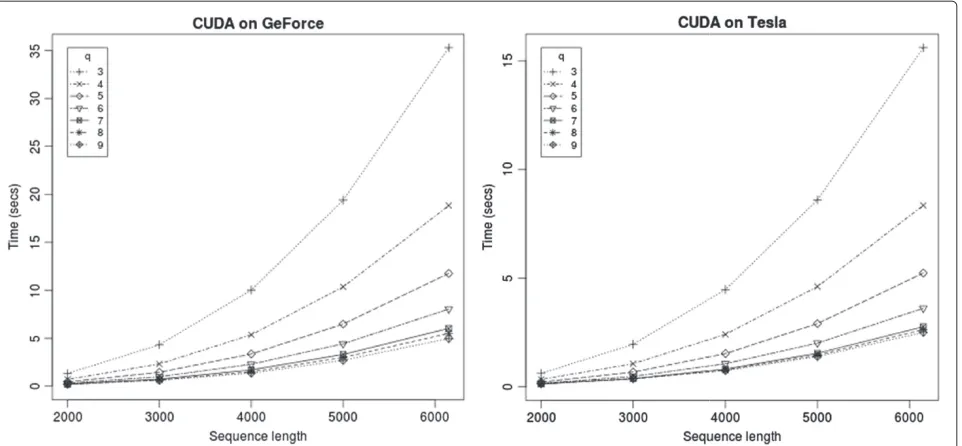
Figure 3Running time of the CUDA program on two GPUs.The programs run twice as fast on the Tesla card than the GeForce card.
The FG algorithm, while faster than Nussinov, was the slowest among the Four-Russians methods, as expected. The completely memoized version was slower than the other two variants. This is because every lookup of the preprocessing table includes a check to see if the pair of vectors has already been processed. There are 22qunique vector pairs but there areO(nq3)queries to the preprocess-ing table and each query involves checkpreprocess-ing if the vector pair has been processed plus the processing time for new pairs. There areO(n2
q2)vector pairs in the table. For larger n (e.g., n > 1000 and q = 8), all the 22q vectors are expected to be present in the DP table. Generally, memo-ized subproblems are relatively expensive compared to the lookup. Since the preprocessing here has onlyqsteps, the advantage of memoization is not seen.
The partially memoized version was slightly slower than the two vector algorithm. Again, the advantage of poten-tially less preprocessing than the two-vector method is erased by the need to check if a vector has been processed. The two-vector method was the fastest on all sequence lengths tested.
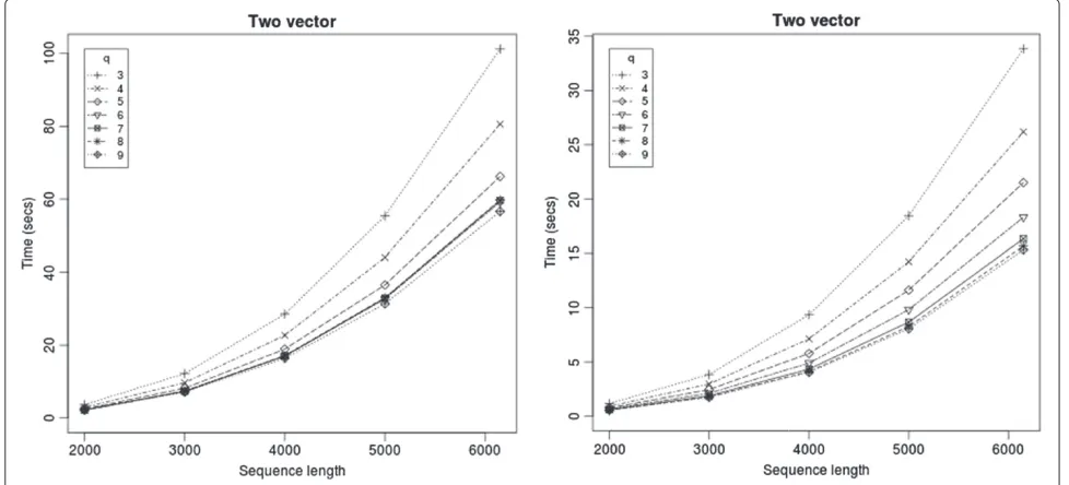
For short sequences the two vector method took negli-gible time (less than 0.2 seconds up to 1000 bases) and are not reported. For longer sequences, we noticed that using longer vector lengths reduced the running time. How-ever the improvement saturated atq=8 or 9 (Figure 2). Beyond this, the extra work in preprocessing overshad-owed the benefit. A similar trend was seen for the memo-ized versions too. However, for the FG methodq=3 gave the best speedup and longer vector lengths had a slower running time due to the extra preprocessing at every group.
The algorithms implemented compute the same match-ings as the Nussinov algorithm. The correctness of each implementation was evaluated by comparing the entried of the DP table of the Nussinov algorithm to the analogous values computed by the faster implementation. All the programs were written in C++ compiled with the highest compiler optimizations. We only discuss the experimental results on a desktop and two GPU cards in this paper.
We measured the running times of the different ver-sions of our serial algorithms on a desktop machine with a Pentium II 3 GHz processor and 1 MB cache. The running times of Nussinov and the speedups of various programs compared to Nussinov are shown in Table 1.
The times reported are an average over 10 sequences of approximately the same lengths. Among the serial pro-grams tested, FG had the slowest running times and two-vector method had the best running times. For sequences of length 6000, the two-vector method takes close to a minute on the desktop. As discussed earlier, the extra steps to check if a vector or a pair of vectors have already been processed takes longer than the benefit of potentially fewer steps needed for preprocessing.
Table 2 Running times for the parallel program (in secs)
Length On GeForce On Tesla
2000 0.20 0.14
3000 0.62 0.38
4000 1.36 0.74
5000 2.70 1.39
On sequences of length 5000 bases, two vector had a 20 times speedup, and FG has a 7 times speedup over the Nussinov program on a desktop machine with a Pentium II 3 GhZ processor and 1 MB cache. On a server with four 64-bit cores of Xeon 2.8 GhZ machines with 8 MB primary cache, the running times of all the programs were faster, but the relative speedup on Nussinov was more drastic than that of other programs. The same relative trends for the Four-Russians programs were seen — two-vector method was faster than the partially memoized problem; the totally memoized version, while faster than the FG algorithm was slower than the other two vari-ants. Figure 2 shows the running times of the two-vector method on the desktop and servers, respectively.
Figure 3 shows the execution times on two GPU cards – GeForce GTX 550 Ti card with 1 GB on-card memory and Tesla C2070 with 5 GB memory. The programs take about a second for sequences up to 4000 bases long, and takes about 5 seconds and 2.5 seconds for sequences of length 6000. The running times for various sequence lengths are shown in Table 2. Even in the parallel implementation, we see the same trend with increasing the vector lengths — there is a marked decrease in running time by increas-ing the vector lengths fromq = 3, and the improvement saturates aroundq=8 (Figure 3).
Details on running times of the other variants can be found in the technical report [29].
Conclusions
We described the two-vector method for using the Four-Russians technique for RNA folding. This method is simpler than the Frid-Gusfield method. It also improves the bound of the parallel algorithm by a logn factor to O(logn2n). We showed two other variants that memoize the preprocessing results. These methods are faster than Nussinov by up to a factor of 20 and the Frid-Gusfield method by a factor of 3.
In the future, it will be interesting to see the applica-tion of the Four-Russians technique for other methods that use energy models with thermodynamic parame-ters. The Frid-Gusfield method has been applied to RNA co-folding [30] and folding with pseudoknots [31] prob-lems; the application of the two-vector method to those problems and its implications are also of interest. It will be interesting to compare our run time with the other improvements over Nussinov, like the boolean matrix multiplication method [1].
Competing interests
The authors declare that they have no competing interests.
Authors’ contributions
BV designed the two-vector algorithm, the memoized algorithms, the parallel algorithm. He also designed and implemented the programs and drafted the manuscript. DG motivated the problem and helped in improving the
manuscript. DG and YF designed the FG algorithm. All authors read and approved the final manuscript.
Acknowledgements
The first-listed author thanks Prof. Norm Matloff for the opportunity to lecture in his class; this project spawned out of that lecture. Thanks also to Prof. John Owens for access to the server with a Tesla card. Thanks to Jim Moersfelder and Vann Teves from Systems Support Staff for help in setting up the CUDA systems.
Received: 4 December 2013 Accepted: 18 February 2014 Published: 6 March 2014
References
1. Akutsu T:Approximation and exact algorithms for RNA secondary structure prediction and recognition of stochastic context-free languages.J Comb Optim1999,3(2–3):321–336.
2. Zakov S, Tsur D, Ziv-Ukelson M:Reducing the worst case running times of a family of RNA and CFG problems, using Valiant’s approach.In WABI.2010:65–77.
3. Arlazarov V, Dinic E, Kronrod M, Faradzev I:On economical construction of the transitive closure of a directed graph (in Russian).Dokl Akad Nauk1970,194(11):1209–1210.
4. Frid Y, Gusfield D:A simple, practical and completeO(n3)-time
algorithm for RNA folding using the Four-Russians Speedup.
Algorithms Mol Biol2010,5:13.
5. Chang DJ, Kimmer C, Ouyang M:Accelerating the Nussinov RNA folding algorithm with CUDA/GPU.InISSPIT.IEEE; 2010:120–125. 6. Rizk G, Lavenier D:GPU accelerated RNA folding algorithm.In
International Conference on, Computational Science, vol. 5544. Edited by Gabrielle A, Nabrzyski J, Seidel E, Albada GD, Dongarra J, Sloot PMA. Berlin Heidelberg: Springer; 2009:1004–1013.
7. Stojanovski M, Gjorgjevikj D, Madjarov G:Parallelization of dynamic programming in Nussinov RNA folding algorithm on the CUDA GPU.
InICT Innovations, vol. 150. Edited by Kocarev L. Berlin Heidelberg: Springer; 2011:279–289.
8. Nussinov R, Pieczenik G, Griggs JR, Kleitman DJ:Algorithms for loop matchings.SIAM J Appl Math1978,35:68–82.
9. Nussinov R, Jacobson AB:Fast algorithm for predicting the secondary structure of single-stranded RNA.PNAS1980,77(11):6309–6313. 10. Zuker M, Stiegler P:Optimal computer folding of large RNA
sequences using thermodynamics and auxiliary information.Nucleic Acids Res1981,9:133–148.
11. Tinoco I, Borer PN, Dengler B, Levine MD, Uhlenbeck OC, Crothers DM, Gralla J:Improved estimation of secondary structure in
ribonucleic-acids.Nat-New Biol1973,246(150):40–41. 12. Mathews DH, Disney MD, Childs JL, Schroeder SJ, Zuker M, Turner:
Incorporating chemical modification constraints into a dynamic programming algorithm for prediction of RNA secondary structure.
PNAS2004,101(19):7287–7292.
13. Markham NR, Zuker M:UNAFold.Bioinformatics2008,453:3–31. 14. Zuker M:Mfold web server for nucleic acid folding and hybridization
prediction.Nucleic Acids Res2003,31(13):3406–3415.
15. Hofacker IL:Vienna RNA secondary structure server.Nucleic Acids Res 2003,31(13):3429–3431.
16. Reuter J, Mathews D:RNAstructure: software for RNA secondary structure prediction and analysis.BMC Bioinformatics2010,
11:129.
17. Durbin R, Eddy SR, Krogh A, Mitchison G:Biological Sequence Analysis.
Probabilistic Models of Proteins and Nucleic Acids:Cambridge University Press; 1998.
18. Dowell R, Eddy S:Evaluation of several lightweight stochastic context-free grammars for RNA secondary structure prediction.BMC Bioinformatics2004,5:71.
19. Lu ZJ, Gloor JW, Mathews DH:Improved RNA secondary structure prediction by maximizing expected pair accuracy.RNA2009,
15(10):1805–1813.
20. Knudsen B, Hein J:Pfold: RNA secondary structure prediction using stochastic context-free grammars.Nucleic Acids Res2003,
21. Do CB, Woods DA, Batzoglou S:CONTRAfold: RNA secondary structure prediction without physics-based models.Bioinformatics2006,
22(14):e90–e98.
22. Ding Y, Lawrence CE:A statistical sampling algorithm for RNA secondary structure prediction.Nucleic Acids Res2003,
31(24):7280–7301.
23. Hamada M, Kiryu H, Sato K, Mituyama T, Asai K:Prediction of RNA secondary structure using generalized centroid estimators.
Bioinformatics2009,25(4):465–473.
24. Andronescu M, Condon A, Hoos HH, Mathews DH, Murphy KP:Efficient parameter estimation for RNA secondary structure prediction.
Bioinformatics2007,23(13):i19–i28.
25. Andronescu M, Condon A, Hoos HH, Mathews DH, Murphy KP:
Computational approaches for RNA energy parameter estimation.
RNA2010,16(12):2304–2318.
26. Zakov S, Goldberg Y, Elhadad M, Ziv-Ukelson M:Rich parameterization improves RNA, structure prediction.InResearch in Computational Molecular Biology (RECOMB), Volume 6577,Lecture Notes in, Computer Science. Edited by Bafna V, Sahinalp SC: Springer; 2011:546–562. 27. Wexler Y, Zilberstein CBZ, Ziv-Ukelson M:A study of accessible motifs
and RNA folding complexity.J Comput Biol2007,14(6):856–872. 28. Backofen R, Tsur D, Zakov S, Ziv-Ukelson M:Sparse RNA folding: time
and space efficient algorithms.J Discrete Algorithms2011,9:12–31. 29. Venkatachalam B, Frid Y, Gusfield D:Faster algorithms for RNA-folding
using the Four-Russians method.UC Davis Technical report 2013. 30. Frid Y, Gusfield D:A worst-case and practical speedup for the RNA
co-folding problem using theFour-Russiansidea.InWABI.2010:1–12. 31. Frid Y, Gusfield D:Speedup of RNA pseudoknotted secondary
structure recurrence computation with the Four-Russians method.
InCOCOA, vol. 7402. Edited by Lin G; 2012:176–187.
doi:10.1186/1748-7188-9-5
Cite this article as:Venkatachalamet al.:Faster algorithms for RNA-folding using the Four-Russians method.Algorithms for Molecular Biology20149:5.
Submit your next manuscript to BioMed Central and take full advantage of:
• Convenient online submission
• Thorough peer review
• No space constraints or color figure charges
• Immediate publication on acceptance
• Inclusion in PubMed, CAS, Scopus and Google Scholar
• Research which is freely available for redistribution