An efficient and accurate GB-SAR imaging
algorithm based on the fractional Fourier transform
Lilong Zou,
Member, IEEE
and Motoyuki Sato,
Fellow, IEEE
Abstract—In this paper, an efficient and accurate imaging algorithm is presented for Ground-Based Synthetic Aperture Radar (GB-SAR) or other radar systems that could be formed by a physical or synthetic linear aperture. The imaging algorithm is based on the fractional Fourier transform for the azimuth compression. A mathematical framework is derived according to the projection of a sample reflectivity image onto the pseudopolar coordinate and its implementation was presented. With the data acquisition geometry and the pseudopolar imaging coordinate, the phase of a point target can be expressed as a quadratic phase exponential. It makes that only one-dimensional fractional Fourier transform is needed for the azimuth compression of the time domain backscatter data for the GB-SAR imaging problem. By further research, the optimal transformation order which represents the spatial frequency changes by the fractional Fourier transform was given subsequently. Taking advantage of this optimal representation, the proposed approach avoids the large calculation that occurs in the time domain back projec-tion (TDBP). Comparing to the far-field pseudopolar format algorithm (FPFA), the accuracy of the proposed algorithm is much improved. Meanwhile, the proposed approach holds the almost same computational cost and complexity as the FPFA. The proposed approach keeps the advantages of the imaging quality of the TDBP and the computational cost of the FPFA that are two important aspects of the GB-SAR applications. Both the numerical simulation and the field GB-SAR experiment show that the algorithm is more suitable for the high precision GB-SAR imaging, especially for the near-field.
Index Terms—Ground based synthetic aperture radar (GB-SAR), imaging algorithm, the fractional Fourier transform (FrFT), near-filed imaging, linear aperture radar
I. INTRODUCTION
G
ROUND-based synthetic aperture radar (GB-SAR) is capable of continuous monitoring, providing high sen-sitivity concerning the terrain deformations. Compared to air- and space-borne SAR, GB-SAR has advantages in the continuous monitoring of targets. Currently, some commercial GB-SAR systems are available. Most of them have a fixed rail of 2m length and a radar sensor moving on the linear rail to acquire SAR data with Ku-band (17GHz) [1][2].In the last ten years, Tohoku University has applied this technology to the post-landslide monitoring, and a vast number of field campaigns has been carried out in Japan [3][4]. Typically, a site monitoring with GB-SAR instruments produces a large number of data which needs to be focused. For example, the post-landslide monitoring site in Kumamoto with one of our polarimetric GB-SAR system produces a total of 35000×4 images in an entire year. Moreover, the real-time monitoring is required for the fast movement and the disaster alarm. In one word, an extremely fast and high-resolution imagingalgorithm is needed for the environmental monitoring by GB-SAR. To cope with the huge volume of data, an accurate focusing algorithm which has more efficient computation is proposed in this paper.This algorithm can also be applied to any radar system which is formed by a physical or synthetic linear aperture.
GB-SAR can be regarded as a linear synthetic aperture radar system. The process of constructing an image from a linear synthetic aperture radar data consists of a two-dimensional compression. First of all, the received echo from each of the acquisition point is compressed.Then the echo is compressed along the azimuth direction by taking advantage of the radar motion in order to synthesize a larger antenna aperture. Nowa-days, many imaging algorithms were developed by concerning different purposes and applications.The algorithms consist of two classes: one is the time domain algorithm, the other is the frequency domain algorithm. The time domain algorithm is, as the name implied, focusing in the time domain. The frequency domain algorithm is done in the frequency domain. Both of them have clear advantages and disadvantages.
The time domain methods base on the fact that they can handle an arbitrary system geometry, however, they are slow. The frequency domain methods base on the fact that they are relatively fast by utilizing the fast Fourier transform (FFT), however, they require the sampling positions to lie uniformly on a straight line. Also, the frequency domain methods need a lot of memories to store and evaluate the 2-dimensional Fourier transforms, and the data must be zero-padded to avoid wrap-around effects from the Fourier transforms. There are different algorithms in both of the main groups, all of them are developed to suit for different types of systems, qualities, speed and other criteria.
fast due to the use of FFTs.
The time domain methods can also be used in this area. If the image scenes are small or the trajectory of the platform deviates much from a straight, there is no point by the FFT-based method. If there is much motion error, the cost of applying for motion compensation and autofocus algorithms using FFTs is so large that the saving of the computational is lost. The delay-and-sum [18]-[19], back projection (BP) [20]-[25] and Kirchhoff migration (KM) [26] are the relevant algorithms in the time domain.
Back projection (BP) is an exact inversion technique and frequently used for the linear aperture radar imaging. It works in both near and far field, which means that the range of the different contributions is important for finding the focusing delays. To implement this method in practice, the available discrete range samples must be interpolated [11]. Usually, the linear interpolation is used. However, it is possible to apply an advanced interpolator at the expense of the increased computation time. Although this algorithm can handle an arbitrary array geometry and make no approximations, except for the interpolation, it has one major drawback. For each aperture and the pixel position, we need to compute the range between the sensor element and the pixel, interpolate in the received signal and finally add the value found in the image matrix. For a small image, the direct back projection is quite efficient and often preferred due to its simplicity and robustness. However, for the image with a large aperture and size, the expense of the processing time is substantially great. Another important issue is that whether the GB-SAR is in the near or the far field of the scene. In the near field, the spherical nature of the wave must be taken into account when focusing. If the range satisfies the criteria [27] which is in the far field of the scene, a highly simplified imaging algo-rithm named far-field pseudopolar format algoalgo-rithm (FPFA) is proposed in [28]. The FPFA method formats the reflectivity map onto the pseudopolar coordinate and tends to minimize the processing cost. This robust algorithm is frequently used for GB-SAR applications, but it is developed for the far-field imaging.
Therefore, the goal of this paper is to present an efficient and accurate imaging algorithm to suitable the GB-SAR appli-cations. In this paper, a mathematical framework to focus the time domain data by the fractional Fourier transform (FrFT) is developed under the assumption of the linear aperture and the pseudopolar coordinate. Then, the optimal transformation order which represents the spatial frequency changes by the fractional Fourier transform was also given. This optimal representation avoids the large calculation which occurs in the time domain back projection (TDBP). Comparing to the FPFA method, the accuracy of the proposed algorithm is much improved. At the same time, we achieve almost the same computational cost and complexity.
This paper is organized as follows. Section II presents the mathematical framework of the imaging algorithm and the optimization focusing condition. In Section II-A, a brief review, the main applications and the current formulation form of the fractional Fourier transform are introduced. In Section II-B, the mathematical formulation of focusing a GB-SAR
image by the FrFT under a pseudopolar coordinate system and the associated coordinate transformations are exhibited. Moreover, the final form of the formulation of the algorithm as an image series is also given in Section II-B. The optimized focusing condition and the optimized rotated angle of the formulation are discussed in Section II-C. Section III presents the comparison of the imaging quality and the computational cost among the TDBP, the FPFA and the proposed approach. The results of an extensive validation of the algorithm with the numerical simulations, the field measurements by GB-SAR data are summarized in Section IV. Finally, the conclusions and the current focus of our research are outlined in Section V.
II. MATHEMATICALFRAMEWORK
A. Fractional Fourier Transform
In this section, a brief overview of the FrFT and its implementation is presented. The FrFT is first introduced in its current form by Namias [29] in 1979, although the principle underlying FrFT can be found in the work of Wiener and Wely in the 1920s. Later, a rigorous formal study of the FrFT was carried out in [30]. In recent years, the FrFT has received much attention due to its extensive applications in optics [31][32], signal processing [33][34], acoustic wave [35], ultrasound quantum mechanics [36] and pattern recognition [37].
By a complex scaling of a multiplication of a quadratic phase exponential in the transformed domain with the Fourier transform, the exact form of the fractional Fourier transform is shown in Namias [29]. The relation between the angleφand the corresponding fractional Fourier transform denoted by
Fφ(u) =p1−jcotφ·
Z ∞
−∞
ejπcotφu2·e−j2πcscφut
·ejπcotφt2·x(t)dt
(1)
where φ ∈ (−π
2,
π
2), t is the time and u represent the
frequency.
Equation (1) forms the basis for the fractional Fourier transform algorithms. Equation (1) can be simplified as the conventional Fourier transform when φis an integer multiple ofπ/2. A physical interpretation of (1) is that it can be realized as a quadratic phase exponential in one domain. The FrFT can transform a signal in the time domain (or in the frequency domain) into the domain between the time and frequency by a rotation.
B. Focusing Formulation
The specificity of the GB-SAR is the limited length of the synthetic aperture size compared with the conventional SAR. In the typical GB-SAR system such as IBIS-L, FASTGBSAR, the linear rail on the Ku-band with the 300 MHz bandwidth is 2 m, which is equivalent to the fixed 0.5 m range resolution. The azimuth resolutionδa depending on the range strongly is defined as:
δa =
λ 2Ls
whereλis the wavelength,Lsis the synthetic aperture length andr is the range distance.
In our model, we set the GB-SAR acquisition geometry as in Fig.1, the platform where the sensor elements are mounted follows a path in the x direction (also called the along-track, the azimuth, the cross-range direction, or the slow time domain). The first step is to calculates the reflected signal from a target at the object coordinates (xp, yp). The position of the transmitting and the receiving antenna on the linear rail is xn−d2,xn+d2, respectively. We suppose that the spacing
dbetween the receiving and the transmitting element is small enough to be ignored. Here xn is marked as the phase center where the transmitting sensor element sends out a pulse. The time domain reflected signal is compressed as D(xn, t) in which the received echo from each acquisition pointxn, where
t is the double route delay. Since the electromagnetic waves travel with a much higher speed than that of the platform,tis also called as the fast time domain. Due to the time domain back projection, the synthesis of a radar image can be achieved by integrating the time domain signal with respect to different radar positionsxn. Therefore, the radar reflectivity map at the pointpis estimated as follows:
P(xp, yp) = Z
D(xn, t)·exp(4πjRn
λ0
)dxn (3)
whereRndenotes the double range to the object in meters and
λ0 denotes the wavelength of the system starting frequency.
In this work, we propose an exact mathematical formulation starting from (3) of focusing a GB-SAR image by the FrFT. For the typical GB-SAR system, the amplitude term of the working frequency bandwidth could be ignored, when it varies slowly along the azimuth with certain range. By assuming the pseudopolar coordinate for the object space, the simplest focusing scheme [28] is obtained which is usually adopted for GB-SAR.
The second step is to find an accurate expression for the distance between the target and the sensor
Rn(xn, xp, yp) =
p
(ρsinθ−xn)2+ (ρcosθ)2
=ρ
s
1−2xnsinθ
ρ +
x2
n ρ .
(4)
Applying the first order Taylor expands, (4) can be rewritten as follows:
Rn(xn, xp, yp)'(ρ−xnsinθ+ x2
n
2ρ) (5)
by the approximation|(2xnsinθ−x2n)/ρ|<1. Therefore, the focusing formation could be rewritten as:
P(ρ, θ) = Z
D(xn, t)·exp(
2πj λ0ρ·((ρ
2sin2θ
−2ρxnsinθ+x2n) + (ρ
2sin2θ+ 2ρ2cos2θ)))dx
n, (6)
P(ρ, θ) = exp(2πjρ
λ0 (1 + cos 2θ))
Z
D(xn, t)·
exp(2πj λ0ρ
(ρsinθ−xn)2)dxn. (7)
When considering that ρsinθ = s1u and xn = s2v, the
focusing formation can be expressed as follows:
P(ρ, θ) =s2·e
j2πρ λ0(1+cos
2θ)
·
Z
D(v, t)
·ejλ20πρ(s
2
1u2−2s1s2uv+s22v2)dv.
(8)
wheres1 ands2 are the real value of the scale parameters.
Finally, we introduce a new parametergto adjust the expo-nential term in the above formation. Until now, the focusing formation can be written as follows:
P(ρ, θ) =s2·ej 2πρ
λ0(2−gsin
2θ)
·
Z
D(v, t)
·ejλ20πρ(gs
2 1u
2−2s
1s2uv+s22v2)dv.
(9)
By comparing this formation with the definition of the FrFT (1), we conclude that P(ρ, θ) is proportional to the FrFT at the positionxn , i.e.,
P(ρ, θ) =A·Fφ(xn
s2
), (10)
with
A= s2·exp( 2πjρ
λ0 (2−gsin 2θ))
√
1−jcotφ . (11)
Here A is a constant for the certain range. Equation (10) holds if and only if
cotφ= 2g·s 2 1
λ0·ρ
, (12)
cscφ= 2s1·s2
λ0·ρ
, (13)
cotφ= 2s 2 2
λ0·ρ
. (14)
Sincecot2φ+ 1 = csc2φ, we obtain
s41= λ 2 0·ρ2
4g(1−g), (15)
which yields
0< g <1. (16)
For a given rangeρand the rotated angleφof the fractional Fourier transform, we notice that the parameters g, |s1| and |s2|are determined uniquely. Equation (12) yields thatcotφ > 0. Therefore, we have
0< φ < π
2. (17)
Fig. 1. GB-SAR acquisition geometry.
Fig. 2. Relationship between the phase of one single target and the position on the linear rail at a certain range.
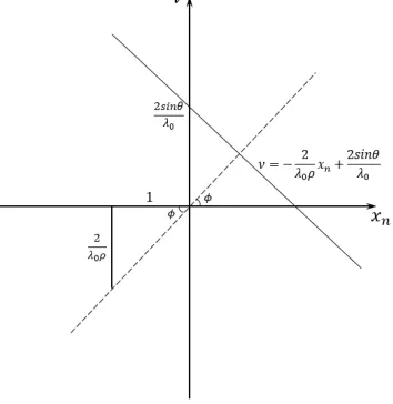
Fig. 3. Geometric interpretation of the relationship between the optimal rotated angle of fractional Fourier transform and the instantaneous spatial frequency.
C. Optimal Focusing Condition
In Section B, we present the proposed mathematical for-mation and the necessary conditions for focusing a GB-SAR image. In this section, we focus on the optimization focusing condition. Furthermore, we compare our computational cost to that of the FPFA.
There is a point target in the line of the sight (LOS) direction
Fig. 4. The optimal rotated angle of the FrFT for a certain range by considering the IBIS-L GB-SAR system.
shown in Fig. 2. At each position along the rail, the point targets contribute to the same amplitude for all the reflections in the range resolution. However, the phase ψ is different slightly for the distance from the antenna to the target. In the case of GB-SAR, the phase ψ at the position xn of the antenna can be expressed as follows:
ψ(xn) =−4π
λ0
·qx2
n+y2p. (18)
The spatial frequencyνare the spatial analog of the angular velocityωand the frequencyf in the time domain of a signal. In this paper, we rewrite the spatial frequencyν with regard to the phase ψin the polar coordinate as follows:
ν(xn) = k(xn)
2π =
1 2π·
dψ(xn)
dxn '
2 sinθ λ0
− 2xn
λ0·ρ
, (19)
where k is the angular wavenumber. Hence the spatial fre-quencyν is linear to the antenna position for a certain range. As the range increasing, the difference of the instantaneous spatial frequency at different antenna position decrease. And the variety of this spatial frequency will produce a greater blur in the traditional Fourier based focusing algorithm. However, the distribution of the above linear spatial frequency has the narrowest representation in the fractional domain. Thus, by finding the optimal rotated angleφof the FrFT we can provide a highly focused response in the azimuth direction of a certain range signal.
The solid line in Fig.3 indicates the variety of the spatial frequency at different antenna position xn. As the axis (the dashed line) rotates to a position perpendicular to the solid line, then the magnitude response reaches the maximum value. For the simplest case, the optimal angle is defined as follows:
φopt= tan−1(λ0·ρ
2 ). (20)
From an observation of the real GB-SAR, the data is discrete along the linear rail. Using the interpretation shown in Fig.3 we obtain
φopt= tan−1(
∆ν·λ0·ρ
2∆xn ), (21)
of the acquisition points along the linear rail. Since ∆ν = ∆xn/N, we have
φopt=tan−1( λ0·ρ 2N·∆x2
n
). (22)
Equation (22) shows the optimal rotated angle of the FrFT for a certain range of the GB-SAR data, which means that we can get an an optimal rotated angle by (22) for any range of the data in the GB-SAR observation. The optimal rotated angle is determined by the starting frequency, the size of the step and the number of the acquisition of the GB-SAR system setting. Moreover, it is also determined by the slant range. Using the optimal rotated angles with (11)-(13), the parameters
s1,s2 andgwhich are used to focus a GB-SAR image by the proposed FrFT approach can be calculated.
The distance of the range from the radar to any arbitrary points within the image scene is denoted as ρ0. Then the far field criteria of the radar aperture is
ρ0 >2L
2
λc , (23)
where λc is the wavelength at the center frequency of the radar. For a typical commercial GB-SAR system working at Ku-band with 5mm step size along the 2 m linear rail, the far field criteria is around 460m. The optimal rotated angle calculated by (22) is presented in Fig.4. The rotated angle changes from 0 to 90 degree until the range distance reach the criteria.When the range distance satisfies the far field criteria, the proposed approach match to the FPFA.
III. IMAGEQUALITY ANDCOMPUTATIONALCOST
This section presents the performance of our proposed ap-proach. The quantitative analysis is carried out from the quality of the images and the speed of the algorithm. Moreover, we compare our algorithm with the TDBP and the FPFA.
A. Image Quality
It is important to establish the GB-SAR image quality in different imaging algorithms. There are several measures used to judge the quality of an image.In this paper, we focus on the point spread functions in the azimuth direction, and calculate the peak to the sidelobe ratio (PSLR) and the integrated sidelobe ratio (ISLR). PSLR is the ratio between the peak of the main lobe and that of the most prominent side lobes [38]. ISLR is defined as the ratio between the energy of the main lobe and that integrated over all the side lobes [39].Both sides of the main lobe in azimuth direction in a range resolution, are calculated in this paper. Since the extent of the scene is limited, we typically integrate over several (5 to 10) lobes on both sides of the main one.
In the following simulations, we compare our approach to two different algorithm on the imaging of one reflector: the TDBP and the FPFA. The position of the reflector changes from 3 m to 500 m in range. The parameters of a real GB-SAR system are used in the simulations. Figure 5 and 6 show PSLR and ISLR of the reflector for the TDPB, the FPFA and the proposed approach, respectively. For the proposed
Fig. 5. Peak to side lobe ratio of the TDBP, the FPFA and the proposed approach.
Fig. 6. Integrated side lobe ratio of the TDBP, the FPFA and the proposed approach.
approach, the criteria |(2xnsinθ−x2n)/ρ| is approximately 10 m in range. When the slant range satisfies the criteria, PSLR (≈ −29dB) and ISLR (≈ −18dB) do not change much between the proposed approach and the TDBP. Notably, PSLR and ISLR of the FPFA move close to that of the TDBP with the range increasing until to the far field condition. Therefore, when the target position satisfies the approximated criteria, the image quality by the proposed approach shows the main lobe equally comparing to that of the TDBP. It is worth mentioning that the criteria satisfies most of the application conditions. Now, the typical criteria given for the current commercial GB-SAR system is around 10 m.
B. Computational Cost
The synthesis of an entire reflectivity image using (3) has associate a high computational cost defined by O(N N0M0), whereM0 andN0 denote the number of pixels in thexandy
directions, respectively.N denotes the acquisition point along the linear rail. In practice, the TDBP need the interpolation before the azimuth compression. Typically, an FFT with zero padding will be used.
Fig. 7. Computation time of the TDBP, the FPFA and the proposed approach.
signals from the frequency domain to the time domain.Then 1-D fractional Fourier transform need to be used for the azimuth compression. Ozaktas (1996) [40] presented an efficient and accurate computation algorithm of the FrFT which has the same computational cost as the FFT. In the proposed approach, the total computational cost from the raw data to the image is O(M N logM N+M(N + 4)). Here M is the number of the frequency points and N is the number of the acquisition points along the linear rail.O(M N logM N)is the sum of the computational cost in 1-D FFT for the range compression and 1-D fractional Fourier transform for the azimuth compression. AndO(M(N+4))is the computational cost for the calculation of the parameters. When the parameters are given fixed, we use them repeatedly for a GB-SAR measurement with the fixed acquisition parameters. For example, if we focus a real GB-SAR measurement with the scene size of 500 m in the range and 400 m in the azimuth, the computational cost of the proposed approach is 50 times lower than that of the TDBP. However, for the FPFA, no parameters need to be calculated beforehand and the computational cost isO(M N logM N).
To test the computational cost of the algorithms, we use an Inter(R) Core(TM) i7-6700 [email protected] with 32GB RAM Desktop PC with MATLAB. The results of the simulations are shown in Fig. 7, which show the comparison for different size of the scene focusing by the TDBP, the FPFA and the proposed FrFT algorithm presented in Section B.The proposed FrFT approach save much more time than the TDBP which can be observed in Fig. 7. However, the proposed FrFT approach costs more computational time than the FPFA. That is due to two factors: first, the parameters in the proposed FrFT approach do not appear in the FPFA. Second, the Fourier transform function in the FPFA is more efficient in MATLAB. Up to now, we have proved that the proposed FrFT approach can improve the computational cost comparing to the TDBP.
IV. RESULTS
The previous section analyzed the performance and the accuracy of our proposed FrFT algorithm. In this section, the efficiency of our algorithm is analyzed using both the numeri-cal simulation and the field experiment. Moreover, we compare
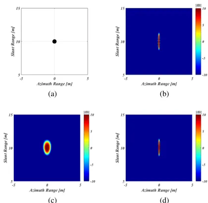
(a) (b)
(c) (d)
Fig. 8. Simulation model and focused GB-SAR image by different methods; (a) a point target located at 10 m in range; (b) the TDBP; (c) the FPFA; (d) the proposed approach.
Fig. 9. Azimuth cuts of reflectivity image at range 10 m obtained by the TDBP, the FPFA and the proposed approach, respectively.
the quality of the focused images obtained by the proposed FrFT approach, the TDBP, and the FPFA, respectively.
A. Numerical Simulation
The parameters of the simulation are given the same as the real GB-SAR system. The radar system operates at 17 GHz (Ku-band) carry frequency and 300MHz bandwidth and the aperture size is 2 m. Before focusing the image, Hanning window function has been applied to the data both in the fre-quency domain and the time domain. The reflectivity images using the TDBP, the FPFA, and the proposed FrFT approach are obtained, respectively.
Fig. 10. GB-SAR observation at Kawauchi Campus, Tohoku University. The red vector indicate the trihedral corner reflector.
TABLE I
SPECIFICATIONS OFIBIS-L GB-SAR SYSTEM
Parameter Value
Central Frequencyf 17.175 GHz
Central Wavelengthλ 17.44 mm
BandwidthB 300 MHz
Scan LengthLs 2 m
Scan time∆t 5 min
Maximum DistanceRmax 4000 m Range Resolutionδr 0.5 m
Cross-Range Resolutionδc 4.4 mrad (0.44m m at 100 m range)
approach is well focused. We investigate the result by cutting the azimuth of the reflectivity image at 10 m range as shown in Fig. 9. It can be observed that the azimuth resolution of the point scatter focused by the proposed approach shows small differences to that by the TDBP. Therefore, the results clearly show that the proposed approach is an excellent method.
B. GB-SAR Measurement
Also, the algorithm is tested on the data of the real experi-ment acquired by IBIS-L GB-SAR system. The site is located at the Kawauchi campus of Tohoku University, Sendai, Japan, as shown in Fig.10. The IBIS-L GB-SAR system used in this study features two horn antennas, one for transmitting and the other for receiving, both with vertical polarization. The system operates in the Ku-band with the center frequency of 17.175 GHz and the bandwidth of 300 MHz. The radar is a stepped-frequency system with variable frequency sampling points that are determined on the basis of the observational range. The entire radar-and-antenna assembly is mounted on a linear rail and it scans about 2 m repeatedly. The 2 m scan spends two minutes and it is repeated every 5 minutes. The system acquires data every 5mm along a 2m scan length at 401 azimuth positions. The rest parameters of the system are summarized in Table I.
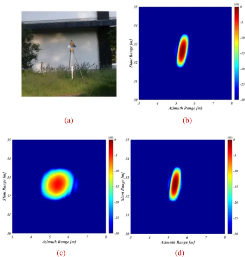
(a) (b)
(c) (d)
Fig. 12. Trihedral Corner Reflector and focused image by different methods; (a) a trihedral corner reflector; (b) the TDBP; (c) the FPFA; (d) the proposed approach.
Fig. 13. Azimuth cuts of reflectivity image at range 30 m obtained by the TDBP, the FPFA and the proposed approach, respectively.
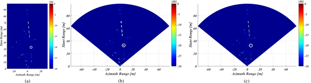
(a) (b) (c) Fig. 11. Focused GB-SAR image by different methods; (a) the TDBP; (b) the FPFA; (c) the proposed approach.
range approximations do not hold for the target position here considered.
V. CONCLUSION
In this paper, we report an efficient and accurate imaging algorithm for GB-SAR. The algorithm is suitable for any radar systems that could form as a physical or synthetic linear aperture. This technique is a type of modified time domain back projection and focuses on the reflectivity map of a polar coordinate. By purely considering the geometrical coordinate and the spatial phase of a fixed target in the linear antenna aperture, it is clearly shown that the azimuth phase mecha-nism could be realized as a quadratic phase exponential. The quadratic phase exponential satisfies the form of the fractional Fourier transforms so that only the 1-D fractional Fourier transform is required to the azimuth compression. Relies on the geometry of the imaging scenario, the spatial frequency along the line rail which is related to the quadratic phase exponential can be optimally represented by the fractional Fourier transform with a certain rotated angle. Considering the real GB-SAR system acquisition parameters, the optimal focusing condition is also given in this paper. Moreover, we compare our algorithm from the imaging quality and the computational cost. Compared with the TDBP, the proposed approach obtained almost the same imaging quality, while the computational cost is extremely low. Compared to the FPFA, computational cost of the proposed approach is almost identical, while the proposed approach also provide accurate imaging results, especially in the near-field. The numerical simulations and the field GB-SAR experiments show that the accurate image can be obtained by the proposed approach no matter in the near- or the far-field. Furthermore, our approach has lower computational cost, which is an important requirement for the GB-SAR applications.
REFERENCES
[1] O. Monserrat, M. Crosetto, and G. Luzi, “A review of ground-based sar interferometry for deformation measurement,”ISPRS J. Photogramm. Remote Sens., vol. 93, pp. 40–48, Jul. 2014.
[2] S. Rodelsperger, A. Coccia, D. Vicente, C. Trampuz, and A. Meta, “The Novel fastGBSARSensor: Deformation Monitoring for Dike Failure Prediction,” inAPSAR 2013, Tsukuba,Japan, Sep. 2013, pp. 23–27.
[3] L. Zou, K. Takahashi, and M. Sato, “Displacement measurement and monitoring with GB-SAR; case study at Aratozawa,” in Proc. of Microwave Conference(APMC), 2014 Asia-Pacific, Sendai, Japan, Nov. 2014, pp. 1022–1024.
[4] K. Takahashi, M. Matsumoto, and M. Sato, “Continuous Observation of Nature-Disaster-Affected areas using Ground-Based SAR Interferome-try,”IEEE J. Sel. Topics Appl. Earth Observ. Remote Sens., vol. 6, no. 3, pp. 1286–1294, 2013.
[5] D. C. Munson and R. L. Visentin, “A Signal processing view of stripmapping synthetic aperture radar,” IEEE Trans. Acoust., Speech, Signal Process., vol. 37, no. 12, pp. 2131–2147, Dec. 1989.
[6] C. Cafforio, C. Prati, and F. Rocca, “SAR data focusing using seismic migration techniques,”IEEE Trans. Aerosp. Electron. Syst., vol. 27, pp. 194–207, Feb. 1991.
[7] A. Li, “Algorithms for the implementation of Stolt interpolation in SAR processing,” inProc. IEEE IGARSS, Houston, Unite State, May 1992, pp. 360–362.
[8] I. G. Cumming and F. H. Wong,Digital Processing of Synthetic Aperture Radar Data: Algorithms and Implementation. MA: Norwood: Artech House, 2005.
[9] R. Bamler, “A comparison of range-doppler and wavenumber domain SAR focusing algorithms,”IEEE Trans. Geosci. Remote Sensing, vol. 30, pp. 706–713, July 1992.
[10] A. M. Smith, “A new approach to range-Doppler SAR processing,”Int. J. Remote Sensing, vol. 12, pp. 235–251, 1991.
[11] M. Y. Jin and C. Wu, “A SAR correlation algorithm which accommo-dates large range migration,”IEEE Trans. Geosci. Remote Sensing, vol. GE-22, pp. 592–597, 1984.
[12] R. W. et al., “Focus FMCW SAR data using the wavenumber domain algorithm,” IEEE Trans. Geosci. Remote Sensing, vol. 48, no. 4, pp. 2109–2118, April 2010.
[13] I. G. Cumming, Y. L. Neo, and F. H. Wong, “Interpretations of the OmegaK algorithm and comparisons with other algorithms,” in Proc. IEEE IGARSS, Toulouse, French, July 2003, pp. 1455–1458.
[14] A. M. Guarnieri and S. Scirpoli, “Efficient Wavenumber Domain Focus-ing for Ground-Based SAR,”IEEE Geosci. Remote Sens. Lett., vol. 7, no. 1, pp. 161–165, 2010.
[15] R. K. Raney, H. Runge, R. Bamler, I. Cumming, and F. Wong, “Efficient Wavenumber Domain Focusing for Ground-Based SAR,”IEEE Geosci. Remote Sens. Lett., vol. 7, no. 1, pp. 161–165, 2010.
[16] R. S. A. Moreira, J. Mittermayer, “Extended chirp scaling algorithm for air- and spaceborne SAR data processing in stripmap and ScanSAR imaging modes,” IEEE Trans. Geosci. Remote Sensing, vol. 34, pp. 1123–1136, Sept. 1996.
[17] A. Moreira and Y. Huang, “Airborne SAR processing of highly squinted data using a chirp scaling approach with integrated motion compensa-tion,” IEEE Trans. Geosci. Remote Sensing, vol. 32, pp. 1029–1040, Sept. 1994.
[18] J. McCorkle and M. Rofheart, “An order N2log(N) backprojector algorithm for focusing wide-angle wide-bandwidth arbitrary-motion synthetic aperture radar,” inSPIE AeroSense Conference, April 1996, pp. 8–9.
[20] A. F. Yegulalp, “Fast backprojection algorithm for synthetic aperture radar,” inProc. IEEE Radar Conf., April 1999, pp. 60–64.
[21] K. Knaell and G. Cardillo, “Radar tomography for the generation of three-dimensional images,”Proc. Inst. Elect. Eng.Radar Sonar Navig., vol. 142, no. 2, pp. 54–60, Apr. 1995.
[22] S. Nilsson and L. E. Andersson, “Application of fast back-projection techniques for some inverse problems of synthetic aperture radar,”Proc. SPIE Algorithms Synthetic Aperture Radar Imagery V, vol. 3370, pp. 62–72, Apr. 1998.
[23] L. M. H. Ulander, H. Hellsten, and G. Stenstrom, “Synthetic-aperture radar processing using fast factorized back-projection,” IEEE Trans. Aerosp. Electron. Syst., vol. 39, no. 3, pp. 760–776, Jul. 2003. [24] L. Zhou, C. Huang, and Y. Su, “A fast back-projection algorithm based
on cross correlation for gpr imaging,”IEEE Geosci. Remote Sens. Lett., vol. 9, no. 2, pp. 228–232, Mar. 2012.
[25] C. Cafforio, C. Prati, and F. Rocca, “SAR data focusing using seismic migration techniques,” IEEE Trans. Aerosp. Electron. Syst., vol. 27, no. 2, pp. 194–207, Mar. 1991.
[26] S. Basu and Y. Bresler, “Error analysis and performance optimization of fast hierarchical backprojection algorithms,” IEEE Trans. Image Process., vol. 10, no. 7, pp. 1103–1117, Jul. 2001.
[27] F. M. Henderson and A. J. Lewis, Principles and Applications of Imaging Radar. New York: Wiley, 1998, vol. 2.
[28] J. FortunyGuasch, “A fast and accurate far-field psedopolar format radar imaging algorithm,”IEEE Trans. Geosci. Remote Sens., vol. 47, no. 4, pp. 1187–1196, 2009.
[29] V. Namias, “The fractional order Fourier transform and its application to quantum mechanics,”J. Ins. Math. Appl., vol. 25, no. 3, pp. 241–265, 1980.
[30] A. C. McBride and F. H. Kerr, “On Namias’s fractional Fourier trans-form,”IMA J. Appl. Math, vol. 39, no. 2, pp. 159–175, 1987. [31] A. W. Lohmann, “Image rotation Wigner rotation and the fractional
order Fourier transform,”J. Opt. Soc. Amer. A., vol. 10, pp. 2181–2186, 1993.
[32] D. Mendlovic and H. M. Ozaktas, “Fractional Fourier transforms and their optical implementation 1,”J. Opt. Soc. Amer. A., vol. 10, pp. 1875– 1881, 1993.
[33] L. B. Almeida, “The fractional Fourier transform and time-frequency representations,”IEEE Trans. Signal Processing, vol. 42, pp. 3084–3091, Nov. 1994.
[34] H. M. O. M. F. Erden, M. A. Kutay, “Repeated filtering in consecutive fractional fourier domains and its application to signal restoration,”IEEE Trans. Signal Processing, vol. 47, pp. 1458–1462, May 1999. [35] G. Gonon, O. Richoux, and C. Depollier, “Acoustic Wave Propagation
in a 1-D Lattice: Analysis of Nonlinear Effects by the Fractional Fourier Transform Method,”Signal Process., vol. 83, pp. 2469–2480, 2003. [36] M. Arif, D. M. J. Cowell, and S. Freear, “Pulse compression of harmonic
chirp signals using the fractional fourier transform,”Ultrasound Med. Biol., vol. 36, no. 6, pp. 949–956, 2010.
[37] W. Jin and Y. Zhang, “Color pattern recognition based on the joint fractional Fourier transform correlator,”Chinese Optics Lett., vol. 5, no. 11, pp. 628–631, 2007.
[38] D. Massonnet and J. C. Souyris,Imaging with Synthetic Aperture Radar. Boca Raton: FL: CRC, 2008.
[39] M. A. and J. Marchand, “Sar image quality assessment,”Asoc. Espaola de Teledeteccin Revista de Teledeteccin, vol. 2, pp. 12–18, 1993. [40] H. M. Ozaktas, O. Arikan, M. A. Kutay, and G. Boadagi, “Digital