Volume 2010, Article ID 404137,18pages doi:10.1155/2010/404137
Research Article
Video Enhancement from Multiple Compressed Copies in
Transform Domain
Viet Anh Nguyen,
1Zhenzhong Chen,
2and Yap-Peng Tan
21Division of Information Engineering, School of Electrical and Electronic Engineering, Nanyang Technological University, Block S2, Nanyang Avenue, Singapore 639798
2School of Electrical and Electronic Engineering, Nanyang Technological University, Singapore
Correspondence should be addressed to Viet Anh Nguyen,[email protected]
Received 1 May 2010; Revised 22 July 2010; Accepted 24 September 2010
Academic Editor: Lei Zhang
Copyright © 2010 Viet Anh Nguyen et al. This is an open access article distributed under the Creative Commons Attribution License, which permits unrestricted use, distribution, and reproduction in any medium, provided the original work is properly cited.
Increasingly, we can obtain more than one compressed copy of the same video content with different levels of visual quality over the Internet. As the original source video is not always available, how to choose or derive a video of the best quality from these copies becomes a challenging and interesting problem. In this paper, we address this new research problem by blindly enhancing the quality of the video reconstructed from such multiple compressed copies. The aim is to reconstruct a video that achieves a better quality than any of the available copies. Specifically, we propose to reconstruct each coefficient of the video in the transform domain by using a narrow quantization constraint set derived from the multiple compressed copies together, using a Laplacian or Cauchy distribution model for each AC transform coefficient to minimize the distortion. Analytical and experimental results show the effectiveness of the proposed method.
1. Introduction
Over the past few decades, transform-based coding has been widely used in lossy image and video compression to exploit the spatial correlation of visual signals. Achieving good energy compaction over a wide class of visual signals, block-based discrete cosine transform (DCT) is commonly adopted in most popular video compression standards, including H.261/3/4 and MPEG-1/2/4 [1,2]. While block-based coding can attain good quality at high bit rates, it often suffers from undesirable coding artifacts (such as blocking artifact, ringing noise, and corner outliers) at moderate to-low bit rates. These coding artifacts are mainly due to the error introduced by the quantization/dequantization process, which may result in severe loss in visual quality and fidelity of the reconstructed video.
To alleviate this problem, postprocessing is one of the most promising solutions as it can improve the video quality without the need of changing the encoder structure. Many postprocessing techniques have been proposed to reduce the quantization artifacts of block-based coding. These
include block-boundary postfiltering techniques to smooth the discontinuous in either spatial [3–7] or transform domain [8–13] such as adaptive filtering and wavelet-based filtering. Also proposed are more sophisticated methods that enhance the reconstructed video by using image/video restoration techniques such as iterative methods based on the theory of projection onto convex sets (POCS) or constrained minimization [14–18], maximum a posterior probability estimation approach (MAP) [19–21], and reg-ularized image/video restoration [22–27]. These methods consider the compressed images/videos to be distorted by a codec system and apply restoration techniques to reduce the quantization noises and coding artifacts.
may record the same interesting soccer match or a piece of news from a television channel and encode it in different formats or using different coding parameters to meet their constraints (e.g., transmission bandwidth, storage capacity, etc.) before sharing it over the network. Similarly, one can gain access to many copies of movie trailers or video clips extracted from DVDs, which have exactly the same content but different visual quality.
Employing the existing postprocessing techniques, one can possibly enhance the quality of each of these compressed copies independently from the other copies. However, as the original source video or information on the video quality is not always available, how to obtain the best video from these multiple compressed copies becomes an interesting problem. The problem shares some similarity with the well-known superresolution (SR) restoration problem, which has been addressed intensively in the literature. For example, Gunturk et al. [28, 29] and Segall et al. [30] proposed to reconstruct high-resolution images by using multiple neighboring low-resolution frames of compressed videos. It should be noted that the restoration or enhancement of high-resolution images in SR requires a set of low-resolution observations, which usually contain different but related views of the scene (e.g., images taken from different cameras, view angles, illumination conditions, or even a sequence of frames from a video). What we consider here is, however, to enhance the video quality from multiple compressed copies of the same content (i.e., no spatial variations) with different levels of quantization noise.
In this paper, we address this new research problem by blindly enhancing the quality of the video reconstructed from multiple compressed copies of the same visual content, where existing postprocessing techniques may no longer be suitable nor effective as they usually consider only a single compressed video. Our aim is to reconstruct a video that achieves better quality than any of the available copies. The proposed method is considered to be a “blind” approach as the original source video is not available, and this makes the problem particularly challenging as we donnot definitively know which of the multiple copies, which frame of a copy, and which region of a frame have the best quality.
In our previous work, we have proposed a scheme based on the theory of POCS to improve the video quality from multiple video copies [31]. However, having projected iteratively the reconstructed video onto the quantization constraint sets in the transform domain and the smooth constraint sets in the spatial domain, the method incurs intensively computational complexity. Here, we consider a different approach and propose a fast method to reconstruct the enhanced video in the transform domain. By exploiting the information from the quantization constraint sets and transform coefficient statistics only in the transform domain, the proposed method can provide an enhanced video with better quality than any of the available copies while incurring much lower computational complexity compared with the previous method.
Specifically, we propose to reconstruct each coefficient of the video in the transform domain by using a narrow quan-tization constraint set derived from the multiple compressed
copies and in which the exact value of the coefficient should lie. In addition, a Laplacian or Cauchy distribution model is utilized to further reduce the distortion of each AC transform coefficient. Analytical and experimental results show that the video reconstructed by the proposed method generally yields a distortion smaller than that of any of the compressed copies available. In many scenarios, the proposed method can attain a notable gain in terms of average peak-signal-to-noise ratio (PSNR) compared to the best video from the multiple compressed copies.
The remainder of the paper is organized as follows. Section 2 briefly reviews some key features of transform-based coding in the latest H.264/AVC standard exploited in this paper. Section3 formulates the problem of blindly enhancing the video content from multiple compressed copies and describes the proposed method with the assump-tion that the temporal resoluassump-tions of the available copies are well aligned. An effective method for temporal registration of multiple compressed copies is presented in Section 4. Mathematical analysis and experimental results to justify of the performance of the proposed method are presented in Sections5and6, respectively. In Section7, we conclude the paper by summarizing our main contributions.
2. Brief Overview of H.264/AVC Transform
Many video coding standards, such as H.261/3/4 and MPEG-1/2/4, have been developed and standardized to address the need of efficient storage and delivery of video content. Although the recent video coding standard H.264/AVC has incorporated a number of advanced coding features to achieve its high coding efficiency, it still employs the so-called block-based hybrid video coding approach. The basic algorithm of a hybrid video coding approach makes use of motion-compensated prediction to exploit the temporal statistical dependency, and transform coding to exploit the spatial statistical dependency. In this section, we will review some key features of transform coding through the state-of-the-art video coding standard H.264/AVC, which will be exploited in this paper to demonstrate the effectiveness of the proposed method.
In essence, the existing video coding standards support intracoding and intercoding. While intercoding employs temporal prediction (motion compensation) from previ-ously encoded pictures, intracoding only uses the informa-tion contained in the picture itself. The (either intra- or inter-) prediction residue, which is the difference between the original and the predicted picture, is then transformed, quantized, and coded. Instead of using 8×8 discrete cosine transform (DCT) like in the previous standards (e.g., H.263 and MPEG-1/2/4), a 4×4 integer transform, which basically has the same properties as a 4 × 4 DCT, is applied in H.264/AVC to avoid the mismatch between encoders and decoders.
Letwdenote a 4×4 block. The 4×4 integer transform coefficients ofware defined in H.264/AVC as
W=CfwCTf
Table1: Quantization step size conversion function.
mod(QP, 6) QP2QSTEP
0 0.6250 1 0.6875 2 0.8125 3 0.8750 4 1.0000 5 1.1250
where⊗represents point-to-point multiplication (e.g., each element of (CfwCTf) is multiplied by the element in the same position of matrix Ef), Cf is the forward transformation matrix, and Ef is the forward postscaling factor matrix, which are defined as [32]
Cf =
⎡ ⎢ ⎢ ⎢ ⎢ ⎢ ⎢ ⎣
1 1 1 1
2 1 −1 −2 1 −1 −1 1 1 −2 2 −1
⎤ ⎥ ⎥ ⎥ ⎥ ⎥ ⎥ ⎦
, Ef =
⎡ ⎢ ⎢ ⎢ ⎢ ⎢ ⎢ ⎢ ⎢ ⎢ ⎢ ⎢ ⎢ ⎣ 1 4 1 √ 40 1 4 1 √ 40 1 √ 40 1 10 1 √ 40 1 10 1 4 1 √ 40 1 4 1 √ 40 1 √ 40 1 10 1 √ 40 1 10 ⎤ ⎥ ⎥ ⎥ ⎥ ⎥ ⎥ ⎥ ⎥ ⎥ ⎥ ⎥ ⎥ ⎦ . (2)
Note that if the macroblock is coded in 16 × 16 intra prediction mode, the DC coefficients of the 4 × 4 luma residue blocks will be transformed again using a 4 ×4 Hadamard transform to decorrelate the DC coefficients before the quantization process (see [32] for details).
Let Zi j denote the quantized coefficient value and
Wi j denote the dequantized coefficient value of Wi j. The quantization process in H.264/AVC is defined as follows:
Zi j=sgn
Wi j
×
⎢ ⎢ ⎢ ⎣Wi j
Qi j +g ⎥ ⎥ ⎥ ⎦
Wi j=Zi j×Qi j,
, (3)
where Qi j is the quantization step size, g is the rounding control parameter, · is the floor operator that rounds to the nearest integer towards minus infinity, and sgn(·) returns the sign of a signal. In the implementation of the H.264/AVC reference software [33],g =1/3 for intra blocks and g = 1/6 for interblocks. It should also be noted that the postscaling operation is incorporated together with the forward quantizer in the reference software to avoid rounding errors in the transform process. The quantization step sizeQi jis determined by a quantization parameter (QP), which is calculated by the rate control algorithm and may be different for each macroblock. The quantization step size will double in size for every increment of 6 in QP and increase by 12.5% for each increment of 1 in QP. Mathematically,Qi jcan be computed from QP as
Qi j=QP2QSTEP(mod(QP, 6))2QP/6, (4) where QP2QSTEP function is defined in Table1, and mod (M,N) is the remainder of integer division ofMbyN.
The inverse transform is given by [32]
w=CT i
W⊗Ei
Ci, (5)
whereCiis the inverse transformation matrix, andEiis the inverse postscaling factor matrix, which are defined as
Ci=
⎡ ⎢ ⎢ ⎢ ⎢ ⎢ ⎢ ⎢ ⎢ ⎢ ⎢ ⎢ ⎣
1 1 1 1 2
1 1
2 −1 −1 1 −1
2 −1 1 1 −1 1 −1
2 ⎤ ⎥ ⎥ ⎥ ⎥ ⎥ ⎥ ⎥ ⎥ ⎥ ⎥ ⎥ ⎦
, Ei=
⎡ ⎢ ⎢ ⎢ ⎢ ⎢ ⎢ ⎢ ⎢ ⎢ ⎢ ⎢ ⎢ ⎢ ⎣ 1 4 1 √ 10 1 4 1 √ 10 1 √ 10 2 5 1 √ 10 2 5 1 4 1 √ 10 1 4 1 √ 10 1 √ 10 2 5 1 √ 10 2 5 ⎤ ⎥ ⎥ ⎥ ⎥ ⎥ ⎥ ⎥ ⎥ ⎥ ⎥ ⎥ ⎥ ⎥ ⎦ . (6)
3. Problem Formulation and Proposed Method
We can formulate the problem considered as follows: given Kdifferent compressed copies of the same video content, let Yk(i) andQk(i) denote the quantized (residual) value and the corresponding quantization step size of theith integer trans-form coefficient in a video frame of thekth copy, respectively, and, if any, letPk(i) be the corresponding intraprediction value for intramode or motion-compensated prediction value for intermode in the integer transform domain. Note that the prediction values from the compressed videos are only available in the spatial domain. Hence,Pk(i) is obtained by using the integer transform as defined in (1). The decoded valueXk(i) of theith integer transform coefficient in thekth copy is computed as
Xk(i)=Yk(i)×Qk(i) +Pk(i). (7) The distortion of the decoded frame in terms of mean square error (MSE) can be computed in the transform domain according to Parseval’s Theorem as follows:
msek= 1 N
N
i=1
X(i)−Xk(i)
2
, (8)
whereNis the total number of pixels in the video frame, and X(i) denotes the value of theith integer transform coefficient of the original frame.
LetX(i) be the estimated value of the coe fficient in the enhanced reconstructed video. The objective is to findX(i) givenXk(i)’s andQk(i)’s fromKmultiple compressed copies of the same video content such that the distortion of the reconstructed video is no larger than that of any given copy, that is,
mse= 1 N
N
i=1
X(i)−X(i) 2≤msek, ∀1≤k≤K. (9)
set (QCS), in which the exact value of the coefficient should lie. Different compressed copy will possibly give a different QCS of each coefficient in the video frame. In the simple dead-zone scalar quantization defined by (3), it is easy to see that each QCS of theith integer transform coefficient reveals thatX(i)∈Sk(i)=[αk(i), βk(i)], where
αk(i)=Xk(i)−
1−gQk(i), βk(i)=Xk(i) +
1−gQk(i),
ifYk(i)=0,
αk(i)=Xk(i)−gQk(i), βk(i)=Xk(i) +
1−gQk(i),
ifYk(i)>0,
αk(i)=Xk(i)−
1−gQk(i), βk(i)=Xk(i) +gQk(i),
ifYk(i)<0.
(10)
GivenK compressed copies, we can have up toKdifferent QCSsS1(i),S2(i),. . .,SK(i) in which the exact value of theith integer transform coefficient should lie. Thus, if the frames of theseK different compressed copies are well aligned, we can obtain a narrow QCS forX(i) by taking the intersection of these sets, as follows:
S(i)=α(i),β(i)= K
k=1
Sk(i),
where
⎧ ⎨ ⎩
α(i)=max{αk(i)|1≤k≤K}, β(i)=minβk(i)|1≤k≤K
.
(11)
Equation (11) shows that by having multiple compressed copies, the size of the QCS for each integer transform coefficient can likely be reduced. The reduction in QCS size allows us to estimate a more accurate integer transform coefficient and thus reconstruct a video frame with a lower distortion. Ideally, we can obtain the exact integer transform coefficient if the QCS becomes a scalar, a scenario that rarely occurs. Hence, we propose in this paper to reconstruct each integer transform coefficient by using the corresponding narrow QCS and justify that by doing so the constraints in (9) can be satisfied.
Since each integer transform coefficient is quantized independently by a quantization step size, minimizing the MSE subject to the constraints specified in (9) is equivalent to minimizing the distortion caused by each integer transform coefficient. In order to have a quantization that better fits to a nonuniform distribution of the integer transform coefficient over the QCS, H.264/AVC decoder uses the rounding control parameterg in (3) to control the position of the reconstructed value inside the QCS interval. Due to the nonsymmetric distribution, the reconstructed value is not located in the center of the corresponding QCS like the previous coding standards such as H.263 and MPEG-1/2/4. A fixed value ofg smaller than half of the QCS size is used to reduce the quantization error. However, to achieve the optimal quantization error, the reconstructed value should be adaptively decided based on the probability distribution of the integer transform coefficient over the corresponding QCS.
Consider the ith integer transform coefficient X(i). Let f(x) denote the probability density function (pdf) of that integer transform coefficient. Given a QCSS(i)=[α(i),β(i)] ofX(i), the average distortion incurred by reconstructing the coefficient asX(i) can be computed as
ε(S(i))=
β(i)
α(i)
x−X(i) 2fS(x)dx, (12)
where fS(x) is the pdf ofX(i) over the QCSS(i), which has the form of fS(x) = c f(x). Here,cis the constant so that
Sc f(x)dx=1. It follows thatc=1/
β(i)
α(i) f(x)dxand
ε(S(i))=
β(i)
α(i)
x−X(i) 2f(x)dx
β(i)
α(i) f(x)dx
. (13)
To minimize (13), it is easy to show that (see [34] e.g.,), the reconstructed valueX(i) should be chosen as the centroid of the QCSS(i), given by
X(i)=
β(i)
α(i)x f(x)dx
β(i)
α(i) f(x)dx
. (14)
It has been shown in the previous studies that in the DCT transform domain of a natural image, while the DC coefficients can be approximated as the uniform distribution, the AC coefficient distribution can be modeled by a gener-alized Gaussian [35,36] or Laplacian [37, 38] probability density function. Although the generalized Gaussian model gives the most accurate representation of the AC coefficient distribution, the Laplacian model is commonly employed due to it being more tractable both mathematically and computationally. Recently, Kamaci et al.[39] proposed to use the Cauchy model, which is shown as a better choice than the Laplacian model for estimating the actual probability distribution of AC coefficients in H.264/AVC. In this paper, both Laplacian and Cauchy models will be examined for the estimation of the reconstructed video. In what follows, we present a method to estimate the parameters of both distribution models by using the decoded values from the compressed videos.
Laplacian Model Parameter Estimation. The Laplacian prob-ability density function can be described by
f(x)=b 2e
−b|x|, (15)
wherebis the distribution parameter andxis the coefficient value for a given AC frequency. If the original coefficient values are known, an estimation of parameter b could be computed using the maximum-likelihood (ML) method as
bML=argmax
⎧ ⎨ ⎩log
T
t=1
f(Xt(i))
⎫ ⎬
⎭, (16)
To estimate the Laplacian distribution of each AC coefficient from the dequantized values, we adopt the ML method proposed in [40]. LetX1(i),X2(i),. . .,XT(i) be the dequantized values for a given AC frequency from all the 4 × 4 integer transform blocks of the video frames in theKcompressed copies, andQ1(i),Q2(i),. . .,QT(i) be the corresponding quantization step sizes. Note that the number of dequantized valuesT will be the product of the number of 4×4 integer transform blocks in a video frame and the number of compressed copiesK. LetSt(i)=[αt(i),βt(i)] be the QCS in which the original coefficientXt(i) lies and can be computed using (10). The ML estimate of the parameter bis given by
bML=argmax
⎧ ⎨ ⎩log
T
t=1
PXt(i)
⎫⎬
⎭, (17)
where P(Xt(i)) is the probability of the reconstructed AC coefficient beingXt(i), and it can be computed as
PXt(i)
=
βt(i)
αt(i)
b 2e
−b|x|dx
= ⎧ ⎪ ⎪ ⎪ ⎪ ⎪ ⎪ ⎪ ⎪ ⎪ ⎨ ⎪ ⎪ ⎪ ⎪ ⎪ ⎪ ⎪ ⎪ ⎪ ⎩
1−1 2e
bαt(i)−1
2e −bβt(i),
ifαt(i)<0, βt(i)>0, 1
2sgn(αt(i))
e−b|αt(i)|−e−b|βt(i)|
,
otherwise.
(18)
Substitute (18) into (17), we have
bML=arg max
⎧ ⎨ ⎩
T
t=1,αt(i)βt(i)<0
log
1−1 2e
bαt(i)−1
2e −bβt(i)
+ T
t=1,αt(i)βt(i)≥0
log
!
1
2sgn(αt(i))
×e−b|αt(i)|−e−b|βt(i)|
"#
.
(19)
Differentiate (19) with respect tob, we obtain
T
t=1,αt(i)βt(i)<0
βt(i)e−bβt(i)−αt(i)ebαt(i) 2−ebαt(i)−e−bβt(i)
+ T
t=1,αt(i)βt(i)≥0
βt(i)e−b|βt(i)|− |αt(i)|e−b|αt(i)| e−b|αt(i)|−e−b|βt(i)| =0,
(20)
whose solution can be found by using an iterative root finding algorithm. In our implementation, we used the Newton-Raphon’s root finding method [41].
Cauchy Model Parameter Estimation. The Cauchy probabil-ity densprobabil-ity function can be described by
f(x)= 1 π
b
b2+x2, (21)
whereb is the distribution parameter. Similar to the Lapla-cian model, the parameter b in the Cauchy model can be estimated by the ML method using (17), whereP(Xt(i)) can be computed as
PXt(i)
=
βt(i)
αt(i)
1 π
b b2+x2dx
= 1 π
$
tan−1
%
βt(i) b
&
−tan−1
αt(i) b
'
.
(22)
Substitute (22) into (17), we have
bML=arg max
⎧ ⎨ ⎩
T
t=1
log1 π
$
tan−1
%
βt(i) b
&
−tan−1
αt(i) b
'⎫⎬ ⎭.
(23)
Differentiate (23) with respect tob, we obtain
T
t=1
αt(i)/
b2+α
t(i)2
−βt(i)/
b2+β
t(i)2
tan−1β
t(i)/b
−tan−1(α
t(i)/b) =
0, (24)
whose solution can also be found by using an iterative root finding algorithm. Similar to the case of the Laplacian model, the Newton-Raphon’s root finding method [41] was used in our implementation.
In short, our proposed method for enhancing the video reconstructed from multiple compressed copies can be summarized as follows.
Step 1. Estimate the parameters of the Laplacian and Cauchy distribution for each AC coefficient using (20) and (24), respectively.
Step 2. Obtain the narrow QCS for each integer transform coefficient from the multiple copies using (11).
Step 3. Reconstruct each integer transform coefficient as the centroid of the narrow QCS obtained in Step2using (14).
in H.263 and MPEG-1,2,4). However, in the case of multi-codecs involving only the old coding standards (e.g., multiple compressed videos encoded by H.263 and MPEG-1,2,4), the proposed method can still be applicable.
Complexity Analysis. It is easy to see that the most com-putationally intensive part of the proposed method is to construct the narrow QCS and to estimate the model parameter of the distribution for each AC integer transform frequency. Other than the quantization parameters and quantized values available in the compressed bitstream, the prediction values in the integer transform domain are also needed to compute the narrow QCS, which requires fully decoding every available compressed copy. As only simple and straightforward calculations are required to compute the narrow QCS using (10) and (11) and the reconstructed integer transform coefficient as the centroid of the narrow QCS using (14), this amount of computation is rather insignificant. By applying root-finding algorithms such as the Newton-Raphon’s method, the model parameter estimation for the distribution of each AC integer transform frequency does not require much computation either in comparison with the whole fully decoding process. Thus, the complexity of the proposed method is approximately equal to the complexity required to decode all available compressed input copies.
In addition, in comparison with our previous method [31] or any relevant SR and post-processing methods for quantization error reduction, the proposed method generally requires much less computational complexity. Note that these methods widely employ the constraint-based tech-niques with the popular theory of projection onto convex sets (POCS). One of the necessary constraint sets is the smooth-ness constraint set (SCS) computed in the spatial domain, which also requires fully decoding all the compressed input copies, not to mention the computational load required for the computation of the smoothness criteria. Furthermore, the iterative projection process among various constraint sets requires a number of conversions among the SCS and other constraint sets (e.g., between the spatial domain for the SCS and the transform domain for the QCS), which results in intensively computational load. In order to converge to the optimal solution, a few number of iterations is generally required, which makes the computational complexity of these methods significantly higher compared with that of the proposed method.
4. Video Alignment
In Section 3, we propose an effective method to enhance the reconstructed video from multiple compressed copies of the same video content under the assumption that the frames of the available copies are well aligned. However, this assumption may not always hold in practice. For example, a same broadcast video can be encoded by different people starting at slightly different time instances. The same video may also be edited, encoded at different frame rate (e.g., 3-2 pull down), or subjected to frame dropping during the video compression process.
We propose in this section a simple method to align the given compressed video sequences. Without loss of generality, we focus on the alignment of two video sequences here. LetR= {rn: 1≤n≤NR}andQ= {qn: 1≤n≤NQ} wherernandqnrepresent thenth video frames,NR andNQ
are the total number of frames in the two video sequences. Our objective is to find alignment functionsu(·) (1≤u(n)≤ NR) andv(·) (1≤v(n)≤NQ) such that frameru(n)is similar
to frameqv(n), for 1≤n≤NT, whereNTis the total number
of possible matching frame pairs. Mathematically, finding the optimal alignment functions u(·) andv(·) is equivalent to minimizing the matching cost function defined as
C(R,Q)=min
u,v
NT
n=1
w(u(n),v(n))·dru(n),qv(n)
, (25)
where d(ru(n),qv(n)) is the distance function representing
the difference or dissimilarity between frame ru(n) and
qv(n), w(·,·) is the weighting function which could place
different emphasis on different aligned frame pairs, and
(NT
n=1w(u(n),v(n)) = 1. Frame ru(n) is considered similar
to frameqv(n) if their frame distance measured(ru(n),qv(n))
is sufficiently small. In addition, it should be noted that the minimization is subject to a causal constraint onu(·) and v(·) that is u(n) ≤ u(n+ 1) and v(n) ≤ v(n+ 1) with 1≤n≤NT.
It can be seen that the accuracy of the alignment will partly depend on how efficiently the frame distance measure d(·,·) is able to differentiate dissimilar frames. Many sophisticated frame distance measures have been proposed in the literature for image/video matching, as color histogram, image signatures, and so forth. Since compressed copies of the same video content exhibit no spatial variations such as different view angles or illumination conditions like the case of existing image/video matching problems, we use here a simple but effective frame distance measure based on the side information extracted from the compressed videos.
LetS(i) be the narrow QCS of theith integer transform coefficient obtained from frame ru(n) and qv(n) using (11).
The proposed frame distance measure between frameru(n)
andqv(n)is defined as
dru(n),qv(n)
= N
i=1
h(S(i)), withh(S(i))=
⎧ ⎨ ⎩
1, ifS(i)=φ, 0, ifS(i)=/φ,
(26)
0 1000 2000 3000 4000 5000 6000 7000 8000
Distanc
e
0 10 20 30 40 50 60 70 80 90 100 Frame number
Distance from frame 30 Distance from frame 50
Figure1: The distance from frames 30 and 50 of one compressed copy to all frames of the other compressed copy of a short video segment from a popular situation comedy.
distance measure is smaller than some threshold, which is empirically obtained by simulation with a large number of video sequences.
To solve (25), we use the forward dynamic programming technique proposed in [42] for video retrieval. Let C(i,j) is the minimum matching cost between two subsequences Ri = {rn : 1 ≤ n ≤ i}and Qj = {qn : 1 ≤ n ≤ j}. The minimum costC(i,j) for all 1≤i≤NRand 1≤j≤NQcan be computed by using the recursive formula given by
Ci,j=min
⎧ ⎪ ⎪ ⎪ ⎪ ⎪ ⎪ ⎪ ⎨ ⎪ ⎪ ⎪ ⎪ ⎪ ⎪ ⎪ ⎩
Ci−1,j+ 1 NR+NQ ·
dri,qj
,
Ci−1,j−1+ 2 NR+NQ ·
dri,qj
,
Ci,j−1+ 1 NR+NQ ·
dri,qj
,
(27)
where C(i,j) = ∞ for i = 0 or j = 0. Hence, the matching frame pairs between video sequencesRandQcan be found by determining the optimal path (i.e., the path with minimum final matching costC(NR,NQ)). It should be noted that only frame pairs obtained from the optimal path whose the distance measures are smaller than some predefined threshold will be utilized to enhance the reconstructed video by using the proposed method.
It is easy to see that the most computationally intensive part of the proposed alignment method is to compute the minimum matching cost function C(i,j) using (27). The computation of eachC(i,j) needs only three algebraic operations (each algebraic operation consists of one addition and one multiplication) and two numerical comparisons. Therefore, the optimal path, and hence matching frame pairs between video sequences R and Q, can be obtained withO(NRNQ) algebraic operations andO(NRNQ) numerical comparisons. Thus, the complexity of the proposed align-ment method isO(NRNQ).
Copy 1 Copy 2
Copy 3 α3(i) α2(i)
α1(i)
X3(i)
X2(i)
X1(i)
β3(i) β2(i)
β1(i) Size of narrow QCS
0 X(i)
(a) A narrower QCS cannot be obtained when the quantization step sizes of Copies 1 and 2 are too large compared with that of Copy 3.
Copy 1 Copy 2
Copy 3 α3(i) α2(i) α1(i)
X3(i)
X2(i)
X1(i)
β3(i)
β2(i) β1(i) Size of narrow QCS
0 X(i)
(b) The relative position of each QCS that is partly determined by the prediction value may help to reduce the size of the narrow QCS.
Figure2: The illustration of how narrow the intersection of the multiple QCSs depends not only on the relation among the sizes of QCSs from multiple compressed copies, but also the position of the QCSs’ intervals.
To evaluate the performance of the proposed alignment method, we have conducted the experiment on a large number of test sequences. To create the misalignment among the compressed video inputs, the original video sequence was encoded starting from different time instances. Furthermore, we purposely dropped some video frames randomly from the original test sequence before encoding to obtain a compressed copy. The experimental results show that the proposed method can obtain the matching frame pairs among these misaligned compressed copies with a hundred percent of accuracy.
5. Analytical Justification
We justify in this section that reconstructing integer trans-form coefficients using the narrow QCS can generally yield a lower distortion than that of using only the QCS of any single copy.
Let X be a random variable representing an integer transform coefficient, which can be either uniform (for a DC coefficient) or Laplacian/Cauchy (for an AC coefficient).
0 0.2 0.4 0.6 0.8 1
P
robabilit
y
0 2 4 6 8 10 12 14
Size of quantization constraint set First copyQ1=14, mse=16.73 Proposed withQ2=19, mse=10.69 Proposed withQ2=53, mse=14.79
Figure3: Probability of the sizes of the QCSS1and narrow QCSS obtained by the proposed method for different values ofQ2.
34 36 38 40 42 44 46
PSNR
(dB)
0 50 100 150 200 250 300
Frame number Foreman
Best input copy
Proposed method + Cauchy model Proposed method + Laplacian model
Figure 4: PSNR results (dB) of the best input copy from the two available compressed copies of the Foreman sequence and the reconstructed video obtained by using the proposed method in conjunction with the Laplacian and Cauchy models to approximate the AC coefficient distribution.
Lemma 1. Consider a quantization constraint setS=[α,β), and its subsetS = [α,β)where S ⊂ S(i.e.,α ≤ α and β≤β). Then, for any such subsetS, we haveε(S)< ε(S) Proof. Consider
A=
β
α
x2f(x)dx, B=
β
α
x f(x)dx, C=
β
α f(x)dx
(28)
as the functions ofβ. Then,ε(S) is also a function ofβand can be easily obtained asε(S,β) = A/C−B2/C2. We first
prove thatε(S,β) is an increasing function ofβby showing ∂ε(S,β)/∂β ≥ 0. Rearrangingε(S,β) as (AC−B2)·(1/C2)
and taking the derivative of the above function with respect toβ, we have
∂εS,β
∂β =(A
C+AC−2BB)1 C2+
AC−B2−2C
C3 .
(29)
Using the Leibniz integral rule, it is easy to see that
∂A ∂β =β
2fβ, ∂B
∂β =β f
β, ∂C
∂β = f
β. (30)
Replacing (30) into (29), we obtain
∂εS,β
∂β =
β2f C+A f −2β f B 1 C2 −2
AC−B2 f C3
=β2C2−AC−2βBC+ 2B2 f
C3.
(31)
Let
Iβ=β2C2−AC−2BCβ+ 2B2. (32) Showing (∂ε(S,β)/∂β) ≥ 0 is equivalent to show I(β) ≥ 0. Taking the first and the second derivatives of I(β) with respect toβ, we have
Iβ=2βC2+β22C f −β2f C−A f
−2f Cβ2+B f β+BC+ 4Bβ f
=2βC2−β2f C−A f −2BC+ 2Bβ f =2CCβ−B+ f2Bβ−β2C−A, Iβ=2fCβ−B+ 2Cβ f +C−β f
+ f2Bβ−β2C−A+ f2B−2βC =2C2+ f2Bβ−β2C−A.
(33)
Since f is a symmetric function, we only need to consider β≥0. LetJ(β)=2Bβ−β2C−A. It is easy to see thatJ(β)= −2(βC−B)≤0. Hence,J(β) is a decreasing function with the increase ofβ. It follows thatJ(β) ≤J(β =α) = 0 and f ≤ 0, henceI(β) ≥0. Thus,I(β) increases withβ, and I(β) ≥ I(β = α) = 0. This leads toI(β) increasing with βtoo, andI(β) ≥ I(β = α) = 0. Similarly, we can prove thatε(S) is a decreasing function ofα. Hence, the assertion in Lemma1holds.
Copy 1: set 2 (33.54 dB)
(a)
Copy 2: set 2 (34.88 dB)
(b)
Copy 3: set 2 (36.43 dB)
(c)
Proposed method (37.53 dB)
(d)
Figure5: The 63th frame from the Stefan sequence obtained by the proposed method and by reconstructing from three input copies.
from the multiple copies, we can reconstruct a video which has a lower distortion, on average, than the video decoded from any given compressed copy.
Furthermore, one would expect that more decrease in distortion can be achieved when the size of the narrow QCS decreases. However, how narrow the intersection of the multiple QCSs depends not only on the relation among the sizes of QCSs from multiple compressed copies, which are determined by the corresponding quantization step sizes, but also the position of the QCSs’ intervals. In particular, we can unlikely obtain a narrower QCS through intersection when the quantization step sizes are not close to each other. For example, if the quantization step size of one copy is too large compared to another, there is a high probability that the QCS interval determined by the smaller quantization step size is entirely confined by the other QCS interval. In this case, we cannot obtain through intersection a QCS narrower than that of the copy with the smaller quantization step size, resulting in no reduction in distortion compared with that copy. Figure 2(a) illustrates this scenario where the quantization step sizes of Copy 1 and 2 are too large compared with that of Copy 3. This happens when the Copy 3 is compressed at much higher quality than the other copies. As a result, we could not obtain a narrower
QCS compared with that of Copy 3, which leads to that the quality of the reconstructed video is not better than that of Copy 3. However, it can be seen in Figure2(b)the relative positions among multiple QCSs can help to reduce the size of the narrow QCS significantly. This is because the position of each independent QCS is partly determined by the prediction value (see (7)), which can be much different for each compressed copy. In addition, one would also expect intuitively the size of the intersected QCS will decrease when more compressed copies are available.
To further illustrate this insight, we provide a simple example. Consider two compressed copies of an integer transform coefficient X, which are coded using two dif-ferent quantization step sizes Q1 and Q2, respectively. We
extensively sampled the values of X based on a Laplacian distribution and quantized withQ1 = 14 and two different
values ofQ2 =19 and 53. AsQ1is not larger thanQ2, it is
obvious that the coefficient reconstructed from the first copy will have a lower distortion. Figure3shows the probability histograms of the sizes of the QCS from the first copy and the narrow QCS obtained through intersection with different values ofQ2. As can be seen from the figure, whenQ2is too
large compared toQ1(e.g.,Q2 = 53), most of the narrow
Copy 1 : set 2 (33.54 dB) Copy 2 : set 2 (34.88 dB)
Copy 3 : set 2 (36.43 dB) Proposed method (37.53 dB)
Figure6: Enlarged regions of the 63th frame from the Stefan sequence obtained by the proposed method and by reconstructing from three input copies for better visualization of the perceptual differences.
Table2: Standard test video sequences.
Sequence No. of frames
Flower 300
Silent 300
Foreman 300
Mother & Daughter 300
Coastguard 300
News 300
Stefan 300
Tempete 250
Tennis 150
Mobile 300
the first copy, resulting in not much distortion reduction. More narrow QCS with smaller sizes compared to that of the first copy can be obtained whenQ2 is close toQ1. This
explains why usingQ2of 19 can yield a lower distortion than
usingQ2of 53 (see Figure3).
6. Experimental Results
We have conducted a series of experiments to evaluate the performance of the proposed enhancement method. Our test sequences include ten popular CIF resolution (352×288) sequences, as shown in Table 2. These sequences contain different amounts of motion and spatial details, and have been widely tested in the literature of video compression.
Copy 1 : set 2 (31.91 dB)
(a)
Copy 2 : set 2 (33.09 dB)
(b)
Copy 3 : set 2 (29.37 dB)
(c)
Proposed method (33.63 dB)
(d)
Figure7: The 77th frame from the Stefan sequence obtained by the proposed method and by reconstructing from three input copies.
compressed in different ways, resulting in various possible performance gains.
6.1. Laplacian and Cauchy Probability Distribution Model. In the first set of the experiments, we evaluate the performance of the proposed method using the Laplacian and Cauchy models, respectively, to resemble the probability distribution of the AC coefficients. We obtained two compressed copies of the Foreman test sequence by encoding at target bit rates 900 kbits/s and 1000 kbits/s. The GOP of the first copy consists of ten frames with one bidirectional-predictive-coded (B) frame between I and P frames, while the GOP of the second copy consists of twelve frames with two bidirectional-predictive-coded (B) frames between I and P frames. Figure 4 shows the PSNR results of the best input copy, which is the copy compressed at 1000 kbits/s in this case, and the reconstructed video obtained by the proposed method using the Laplacian and Cauchy models, respectively. As can be seen from the figure, the proposed method can consistently reconstruct a video which has a better quality than that of the best input copy. However, the proposed method with the Cauchy model can provide a slightly better reconstructed video quality than that of using the Laplacian model. The superiority of the Cauchy model was also
observed on the simulation results of other test sequences. Thus, the Cauchy model is selected to approximate the probability density function of the AC coefficients in our work.
6.2. Multiple Copies Compressed at Different Target Bit Rates. In the second set of experiments, the same video contents of the test sequences were encoded at different target bit rates. We considered two input sets at different bit rate ranges, each consisting of three compressed copies of the same content (see Table3). For the purpose of comparison, we consider two cases where the video frames from the available copies at the same instance are encoded using the same picture coding types I, P, or B frame (Case 1) or different picture coding types (Case 2). The compressed video copies have different GOP structures as shown in Table3.
Copy 1 : set 2 (31.91 dB) Copy 2 : set2 (33.09 dB)
Copy 3 : set 2 (29.37 dB) Proposed method (33.63 dB)
Figure8: Enlarged regions of the 77th frame from the Stefan sequence obtained by the proposed method and by reconstructing from three input copies for better visualization of the perceptual differences.
Table3: Coding parameters of the standard test video sequences.
Video copy no. Target bitrate (kbits/s) GOP structure
Set 1 Set 2 Case 1 Case 2
1 400 700 M=1,N=10 M=0,N=9
2 600 900 M=1,N=10 M=1,N=10
3 800 1000 M=1,N=10 M=2,N=12
∗Nis the number of frames in a GOP,Mis the number of frames between I & P frames.
has a better quality (in terms of average PSNR) than that of any input copy. When the input copies are encoded at high-bit rate ranges or more copies are available, the improvement in quality becomes more significant. Specifically, by using all the three copies in Set 2, the video reconstructed by the proposed method can achieve about more than 1.0-dB
PSNR improvement than that of the best input copy. In some specific test sequences such as Stefan and Coastguard, the PSNR gain can be more than 2.0 dB (see Table5).
Table4: Average PSNR results (in dB) of the best input copy and the video reconstructed by the proposed method from multiple input copies compressed with the same GOP structure at different target bit rates.
Sequence No. of copies 400–600–800 (kbits/s) 700–900–1000 (kbits/s) Best copy Proposed Gain Best copy Proposed Gain
Foreman 2 37.19 37.49 0.30 38.93 39.48 0.55
3 38.42 38.99 0.57 39.37 40.33 0.96
Mobile 2 22.54 22.86 0.32 23.86 24.28 0.43
3 23.37 23.84 0.47 24.85 25.48 0.63
Mother and Daughter 2 43.93 44.28 0.35 45.23 45.79 0.56 3 44.87 45.52 0.65 45.58 46.54 0.97
News 2 42.29 42.62 0.33 44.34 44.88 0.54
3 43.77 44.33 0.56 44.91 45.80 0.89
Silent 2 39.02 39.14 0.12 41.40 41.69 0.29
3 40.72 41.21 0.49 42.03 43.93 0.90
Flower 2 31.18 31.55 0.38 33.03 33.70 0.66
3 32.49 33.22 0.72 33.49 34.65 1.16
Stefan 2 30.45 30.73 0.27 32.49 33.05 0.57
3 31.82 32.43 0.61 32.95 34.08 1.13
Tennis 2 31.45 31.78 0.33 32.75 33.29 0.54
3 32.40 32.97 0.57 32.89 34.17 1.28
Coastguard 2 32.45 32.80 0.35 34.06 34.65 0.59 3 33.58 34.24 0.66 34.43 35.66 1.23
Tempete 2 31.52 31.85 0.32 33.23 33.81 0.58
3 32.74 33.35 0.61 33.59 34.74 1.16
Table5: Average PSNR results (in dB) of the best input copy and the video reconstructed by the proposed method from multiple input copies compressed with different GOP structures at different target bit rates.
Sequence No. of copies 400–600–800 (kbits/s) 700–900–1000 (kbits/s) Best copy Proposed Gain Best copy Proposed Gain
Foreman 2 37.19 37.55 0.36 38.93 39.61 0.68
3 38.41 39.45 1.04 39.45 41.01 1.56
Mobile 2 22.54 23.03 0.49 23.86 25.26 1.40
3 25.12 25.93 0.81 26.65 28.17 1.52
Mother and Daughter 2 43.93 44.30 0.37 45.23 45.87 0.64 3 44.87 45.77 0.90 45.59 46.92 1.33
News 2 42.29 42.51 0.22 44.34 44.78 0.44
3 44.04 44.67 0.63 45.19 46.23 1.04
Silent 2 39.02 39.33 0.31 41.40 41.91 0.51
3 41.33 41.87 0.54 42.66 43.58 0.92
Flower 2 31.18 31.34 0.16 33.03 33.54 0.51
3 32.94 33.87 0.93 33.78 35.44 1.66
Stefan 2 30.45 31.14 0.69 32.49 33.70 1.21
3 31.32 33.01 1.69 32.51 35.02 2.51
Tennis 2 31.45 31.70 0.25 32.75 33.41 0.66
3 32.62 33.48 0.86 33.14 34.65 1.51
Coastguard 2 32.45 32.88 0.43 34.06 34.89 0.83 3 33.42 34.58 1.16 34.23 36.20 1.97
Tempete 2 31.52 31.83 0.31 33.23 33.87 0.64
1.34 1.28 1.16 1.04
2.12
1.99
1.79
1.49
2.59
2.19 2.41
2
2.97 2.78
2.54
2.32
1 1.5 2 2.5 3
PSNR
gain
(dB)
2 3 4 5
Number of copies Foreman
400 kbits/s 600 kbits/s
800 kbits/s 1000 kbits/s
Figure 9: PSNR gain (dB) of the reconstructed video obtained by the proposed method compared with the best input copy of different target bit rates and different number of copies for the Foreman sequence.
as at low-bit rate range, coarse quantization step sizes are generally used for encoding, resulting in a large QCS for each integer transform coefficient. Furthermore, the QCSs of the low-quality copies (e.g., copies 1 and 2 in Set 1) do not contribute much in reducing the size of the narrow QCS obtained by the proposed method. This is because the quantization step sizes used in these copies are generally too large compared to that of the best copy. As a result, the size of the narrow QCS cannot be significantly reduced, and hence it usually remains the same as that of the best copy. Thus, not much quality improvement compared to the best copy can be obtained (see the results of Set 1 in Tables4 and 5 and discussion in Section5). Furthermore, we can generally obtain better PSNR gain in the case where the similar frames from the available copies are coded using different picture coding types (Case 2 in Table5) compared with that of using the same picture coding types (Case 1 in Table4). Note that the size of the narrow QCS depends not only on the relation among the sizes of QCSs from multiple compressed copies, but also the relative position of the QCSs’ intervals. As explained in Section5, this relative position of each independent QCS is partly determined by the prediction value, which can be much different when different picture types are used to code similar frames from the available copies. This will help to reduce the size of the narrow QCS obtained by the proposed method significantly, resulting in more distortion reduction.
In addition, it can be seen from Figure4that the PSNR gains are also quite consistent and uniformly distributed over the entire sequence. For visual comparison, Figures5 and7show the sample frames of the 63th and 77th frames from the Stefan sequence, respectively, which are obtained by the proposed method and by reconstructing from three input copies. The figures show that the proposed method can
0.91 1.071.2 1.26
1.99
1.86
1.63
1.38
2.47
2.29
2.01
1.69
2.83
2.62
2.31
1.93
0.5 1 1.5 2 2.5 3
PSNR
gain
(dB)
2 3 4 5
Number of copies Silent
400 kbits/s 600 kbits/s
800 kbits/s 1000 kbits/s
Figure10: PSNR gain (dB) of the reconstructed video obtained by the proposed method compared with the best input copy of different target bit rates and different number of copies for the Mobile sequence.
achieve a better perceived video quality in terms of sharpness and details compared with those reconstructed from the input copies directly. The perceptual quality differences can be easily noticed in the regions around the player, which are denoted by the rectangular boxes in Figures 5 and 7. For better visualization, these regions are enlarged and shown in Figures6and8, respectively.
Note that the reconstructed frame from the best input copy, in terms of average PSNR, may not always provide better quality than those reconstructed from other copies as shown in Figure 7. However, the reconstructed frame obtained by the proposed method can still achieve better quality, in terms of both PSNR and visual quality, than the best frame reconstructed from the available input copies (i.e., the reconstructed frame from Copy 2 in this case).
6.3. Multiple Copies Compressed at the Same Target Bit Rates. In another set of experiments, the input copies were obtained by encoding the test sequences at the same target bit rates. For simplicity, the same GOP structure was used but with different starting frames for different video copies. This is likely to occur in practice, for example, when different people can encode a same broadcast video but starting at slightly different time instances and upload the compressed videos to websites such as YouTube and Google Video. Thus, the encoded picture type (i.e., I, P, or B) for each particular frame may not be the same among different compressed copies (e.g., it can be an I frame in one copy and a B or P frame in other copies).
Table6: Coding parameters of real video sequences.
Video copy no. Target bitrate (kbits/s) GOP structure
Set 1 Set 2
1 500 900 M=1,N=10
2 700 1100 M=0,N=9
3 900 1300 M=2,N=12
∗Nis the number of frames in a GOP,Mis the distance between I & P frames.
30 32 34 36 38 40
PSNR
(dB)
0 30 60 90 120 150
Frame number Tennis
Copy 1 (variable bit rate) Copy 2 (constant bit rate) Proposed method
Figure 11: PSNR results (dB) of the two copies of the Tennis sequence compressed as variable and constant bit rates and the reconstructed video obtained by using the proposed method.
provide a higher PSNR gain compared with the case in Section 6.2. Specifically, processing the Foreman sequence using three copies encoded at bit rates 400 kbits/s, 600 kbits/s, and 800 kbits/s can only obtain 1.04-dB PSNR gain in comparison with the best copy (see Table 5). Meanwhile, with three compressed copies at 400 kbits/s and 800 kbits/s, we can yield about 1.49 dB and 1.99-dB PSNR gains, respectively. This is because, unlike the case of different bit rates, the quantization step sizes used to code each copy at the same bit rate are quite close to each other. Furthermore, the same video frame in each copy may be encoded with different picture types, resulting in different motion-compensated values. As the quantization interval of a predicted integer transform coefficient is obtained by adding the integer transform value from the reference frame(s), this could effectively reduce the size of the QCS intersection obtained by the proposed method, leading to a large reduction in the distortion. The experimental results also show that more gain can be achieved with the increase of the bit rates and number of input copies.
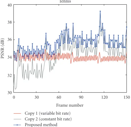
6.4. Multiple Copies Compressed as Variable and Constant Bit Rates. In this set of experiments, we obtained the first
compressed copy of the Tennis sequence by encoding the original video using a constant quantization parameter. The second compressed copy is obtained by encoding at the same target bit rate achieved by the first copy. Unlike the case in Section 6.3, although both copies have the same target bit rate, the first copy that uses the constant QP for the entire video sequence typically obtains a good performance, in terms of both average PSNR and quality consistency. Figure 11 shows the PSNR results of both available compressed copies and the reconstructed video obtained by using the proposed method. It can be seen that although both copies have different quality in terms of average PSNR, the proposed method can still provide a notable PSNR gain compared to that of the first copy like the case in Section6.3. The gain obtained by the proposed method is consistent and uniformly distributed over the entire sequence.
6.5. Application to Real Video Sequences. In the last set of experiments, we evaluate the performance of the proposed method when used together with some real video contents. The real video test sequences were extracted from some featured episodes of a well-known situation comedy with the resolution of 640×480 pixels. The duration of each real video test sequence is about 10 seconds, which consists of about 250 frames. The sample frames of these test sequences are shown in Figure12. The multiple copies of the input video were obtained by encoding these extracted sequences using the coding standard with different target bit rates and coding parameters, which are shown in Table6.
Table 7 shows the average PSNR results of the video reconstructed from multiple video inputs using the proposed method and the best input copy. Like the experiments in Section 6.2, the first two copies in each set were used for the case of two video inputs. Similar to the results obtained by using the standard test sequences, we observe that the proposed method can consistently reconstruct a video which has a better quality than that of the best input copy. Specifically, with the three available compressed copies, the reconstructed video obtained by using the proposed method can obtain about 0.7-dB and 1.2-dB PSNR gains on average for the test sequences in Set 1 and Set 2, respectively.
7. Conclusion
Table7: Average PSNR results (in dB) of the best input copy and the video reconstructed by the proposed method from multiple copies of a situation comedy compressed with different GOP structures and different target bit rates.
Sequence No. of copies 500–700–900 (kbits/s) 900–1100–1300 (kbits/s) Best copy Proposed Gain Best copy Proposed Gain
Ballroom dancing 2 37.48 38.11 0.63 39.51 40.50 0.99
3 39.01 39.78 0.77 40.46 41.74 1.28
Superbowl 2 37.23 38.02 0.79 39.38 40.50 1.12
3 38.96 39.84 0.88 40.40 41.86 1.46
Football 2 36.44 37.11 0.67 38.56 39.65 1.09
3 38.00 38.85 0.85 39.46 40.86 1.40
London 2 36.89 37.44 0.55 38.67 39.60 0.93
3 37.67 38.75 1.08 38.97 40.62 1.65
Routine 2 34.68 34.95 0.27 36.80 37.48 0.68
3 35.50 36.34 0.84 37.21 38.58 1.37
Rugby 2 33.35 33.76 0.41 35.54 36.38 0.84
3 34.82 35.61 0.79 36.51 37.84 1.33
Soldier 2 36.70 37.38 0.68 38.62 39.78 1.16
3 38.44 39.24 0.80 40.63 42.43 1.80
Vegas 2 35.73 36.12 0.39 38.01 38.84 0.83
3 36.86 37.69 0.83 38.57 40.01 1.44
Ballroom Dancing (250) Rugby (200) Superbowl (240) Football (250)
Vegas (250) Soldier (250) London (250) Routine (250)
Figure12: Test sequences (number of frames in parenthesis).
compressed video copies of the same video content with different levels of quality. Without making reference to the original source video or information on the quality of the compressed copies, the proposed method effectively exploits the compressed information of different video copies to reconstruct a video that has a better quality in terms of PSNR than the best compressed copy. Specifically, each coefficient of the reconstructed in the transform domain is estimated using a narrow quantization constraint set obtained from the multiple compressed copies together with a Laplacian or Cauchy distribution model for each AC frequency to minimize the distortion. By reconstructing the enhanced video in the transform domain, the proposed method incurs much lower computational complexity compared with the previous method. In addition, analytical and experimental
results show that the video reconstructed by the proposed method not only yields a lower distortion than any given compressed copy but also achieves a significant PSNR gain compared to the best copy. Furthermore, a similar approach can be easily extended to other transform-based coding schemes such as DCT-based or wavelet-based transform coding.
Acknowledgment
References
[1] H. G. Musmann, P. Pirsch, and H.-J. Grallert, “Advances in picture coding,”Proceedings of the IEEE, vol. 73, no. 4, pp. 523– 548, 1985.
[2] A. N. Netravali and B. G. Haskell,Digital Pictures: Representa-tion and Compression, Plenum Press, New York, NY, USA, 2nd edition, 1995.
[3] H. C. Reeves III and J. S. Lim, “Reduction of blocking effects in image coding,”Optical Engineering, vol. 23, no. 1, pp. 34–37, 1984.
[4] B. Ramamurthi and A. Gersho, “Nonlinear space-variant postprocessing of block coded images,”IEEE Transactions on Acoustics, Speech, and Signal Processing, vol. 34, no. 5, pp. 1258–1268, 1986.
[5] M.-Y. Shen and C.-C. Kuo, “Review of postprocessing tech-niques for compression artifact removal,”Journal of Visual Communication and Image Representation, vol. 9, no. 1, pp. 2– 14, 1998.
[6] K.-K. Kwon, S.-H. Im, and D.-S. Lim, “Deblocking algorithm in MPEG-4 video coding using block boundary characteristics and adaptive filtering,” inProceedings of the IEEE International Conference on Image Processing (ICIP ’05), pp. 541–544, September 2005.
[7] H.-S. Kong, Y. Nie, A. Vetro, H. Sun, and K. E. Barner, “Coding artifacts reduction using edge map guided adaptive and fuzzy filtering,” inProceedings of the IEEE International Conference on Multimedia and Expo (ICME ’04), pp. 1135–1138, June 2004.
[8] T. Chen, H. R. Wu, and B. Qiu, “Adaptive postifiltering of transform coefficients for the reduction of blocking artifacts,” IEEE Transactions on Circuits and Systems for Video Technology, vol. 11, no. 5, pp. 594–602, 2001.
[9] S. Liu and A. C. Bovik, “Efficient DCT-domain blind measure-ment and reduction of blocking artifacts,”IEEE Transactions on Circuits and Systems for Video Technology, vol. 12, no. 12, pp. 1139–1149, 2002.
[10] A. W.-C. Liew and H. Yan, “Blocking artifacts suppression in block-coded images using overcomplete wavelet represen-tation,”IEEE Transactions on Circuits and Systems for Video Technology, vol. 14, no. 4, pp. 450–461, 2004.
[11] Y. Luo and R. K. Ward, “Removing the blocking artifacts of block-based DCT compressed images,”IEEE Transactions on Image Processing, vol. 12, no. 7, pp. 838–842, 2003.
[12] S. Kim and J. Jeong, “Enhancement of wavelet-coded images via novel directional filtering,” inProceedings of the Interna-tional Conference on Neural Networks and Signal Processing, vol. 2, pp. 1062–1065, December 2003.
[13] I. R. Ismaeil and R. K. Ward, “Removal of DCT blocking artifacts using DC and AC filtering,” inProceedings of the IEEE Pacific Rim Conference on Communications Computers and Signal Processing (PACRIM ’03), pp. 229–232, August 2003. [14] R. E. Rosenholtz and A. Zakhor, “Iterative procedures for
reduction of blocking effects in transform image coding,” inImage Processing Algorithms and Techniques II, vol. 1452 of Proceedings of SPIE, pp. 116–126, San Jose, Calif, USA, February 1991.
[15] A. Zakhor, “Iterative procedures for reduction of blocking effects in transform image coding,” IEEE Transactions on Circuits and Systems for Video Technology, vol. 2, no. 1, pp. 91– 95, 1992.
[16] Y. Yang, N. P. Galatsanos, and A. K. Katsaggelos, “Projection-based spatially adaptive reconstruction of block-transform compressed images,”IEEE Transactions on Image Processing, vol. 4, no. 7, pp. 896–908, 1995.
[17] H. Paek, R.-C. Kim, and S.-U. Lee, “On the POCS-based postprocessing technique to reduce the blocking artifacts in transform coded images,”IEEE Transactions on Circuits and Systems for Video Technology, vol. 8, no. 3, pp. 358–367, 1998. [18] O. G. Guleryuz, “Linear, worst-case estimators for denoising
quantization noise in transform coded images,”IEEE Transac-tions on Image Processing, vol. 15, no. 10, pp. 2967–2986, 2006. [19] J. Mateos, A. K. Katsaggelos, and R. Molina, “A Bayesian approach for the estimation and transmission of regular-ization parameters for reducing blocking artifacts,” IEEE Transactions on Image Processing, vol. 9, no. 7, pp. 1200–1215, 2000.
[20] Z. Li and E. J. Delp, “MAP-based post processing of video sequences using 3-D Huber-Markov random field model,” in Proceedings of the IEEE International Conference on Multimedia and Expo (ICME ’02), vol. 1, pp. 153–156, August 2002. [21] J. Li and C.-C. J. Kuo, “Coding artifact removal with multiscale
postprocessing,” inProceedings of the International Conference on Image Processing, vol. 1, pp. 45–48, Santa Barbara, Calif, USA, October 1997.
[22] T. Yang, P. Galatsanos, and A. K. Katsaggelos, “Regularized reconstruction to reduce blocking artifacts of block discrete cosine transform compressed images,”IEEE Transactions on Circuits and Systems for Video Technology, vol. 3, no. 6, pp. 421–432, 1993.
[23] M. G. Choi, Y. Yang, and N. P. Galatsanos, “Multichannel regularized recovery of compressed video sequences,” IEEE Transactions on Circuits and Systems II, vol. 48, no. 4, pp. 376– 387, 2001.
[24] Z. Li and E. J. Delp, “Block artifact reduction using a transform-domain Markov random field model,”IEEE Trans-actions on Circuits and Systems for Video Technology, vol. 15, no. 12, pp. 1583–1593, 2005.
[25] J. J. Zou and H. Yan, “A deblocking method for BDCT compressed images based on adaptive projections,” IEEE Transactions on Circuits and Systems for Video Technology, vol. 15, no. 3, pp. 430–435, 2005.
[26] T. Kartalov, Z. A. Ivanovski, L. Panovski, and L. J. Karam, “An adaptive POCS algorithm for compression artifacts removal,” inProceedings of the 9th International Symposium on Signal Processing and Its Applications (ISSPA ’07), pp. 1–6, February 2007.
[27] A. W.-C. Liew, H. Yan, and N.-F. Law, “POCS-based blocking artifacts suppression using a smoothness constraint set with explicit region modeling,”IEEE Transactions on Circuits and Systems for Video Technology, vol. 15, no. 6, pp. 795–800, 2005. [28] B. K. Gunturk, Y. Altunbasak, and R. M. Mersereau, “Mul-tiframe resolution-enhancement methods for compressed video,”IEEE Signal Processing Letters, vol. 9, no. 6, pp. 170– 174, 2002.
[29] B. K. Gunturk, Y. Altunbasak, and R. M. Mersereau, “Multi-frame blocking-artifact reduction for transform-coded video,” IEEE Transactions on Circuits and Systems for Video Technology, vol. 12, no. 4, pp. 276–282, 2002.
[30] C. A. Segall, R. Molina, and A. K. Katsaggelos, “High-resolution images from low-“High-resolution compressed video,” IEEE Signal Processing Magazine, vol. 20, no. 3, pp. 37–48, 2003.
[31] C. Wang, G. Yang, and Y.-P. Tan, “Reconstructing videos from multiple compressed copies,” IEEE Transactions on Circuits and Systems for Video Technology, vol. 19, no. 9, pp. 1342–1351, 2009.
[33] “JM 12.4-H.264 reference software,” http://iphome.hhi.de/ suehring/tml/.
[34] R. L. de Queiroz, “Processing JPEG-compressed images and documents,”IEEE Transactions on Image Processing, vol. 7, no. 12, pp. 1661–1672, 1998.
[35] F. M¨uller, “Distribution shape of two-dimensional DCT coefficients of natural images,”Electronics Letters, vol. 29, no. 22, pp. 1935–1936, 1993.
[36] T. Eude, R. Grisel, H. Cherifi, and R. Debrie, “On the distribution of the DCT coefficients,” in Proceedings of the IEEE International Conference on Acoustics, Speech, and Signal Processing (ICASSP ’94), vol. 5, pp. 365–368, Adelaide, Aus-tralia, April 1994.
[37] E. Y. Lam and J. W. Goodman, “A mathematical analysis of the DCT coefficient distributions for images,”IEEE Transactions on Image Processing, vol. 9, no. 10, pp. 1661–1666, 2000. [38] S. R. Smoot and L. A. Rowe, “DCT coefficient distributions,”
inHuman Vision and Electronic Imaging, Proceedings of SPIE, pp. 403–411, San Jose, Calif, USA, February 1996.
[39] N. Kamaci, Y. Altunbasak, and R. M. Mersereau, “Frame bit allocation for the H.264/AVC video coder via cauchy-density-based rate and distortion models,”IEEE Transactions on Circuits and Systems for Video Technology, vol. 15, no. 8, pp. 994–1006, 2005.
[40] T. Brand˜ao and M. P. Queluz, “No-reference image quality assessment based on DCT domain statistics,”Signal Processing, vol. 88, no. 4, pp. 822–833, 2008.
[41] C. T. Kelley, Solving Nonlinear Equations with Newton’s Method, Fundamentals of Algorithms, SIAM, Philadelphia, Pa, USA, 2003.