Volume 2011, Article ID 530325,19pages doi:10.1155/2011/530325
Research Article
Automatic Reasoning about Causal Events in Surveillance Video
Neil M. Robertson
1and Ian D. Reid
21School of Engineering and Physical Sciences, Heriot-Watt University, Edinburgh EH14 4AS, UK 2Department Engineering Science, University of Oxford, Oxford OX1 3PJ, UK
Correspondence should be addressed to Neil M. Robertson,[email protected]
Received 1 April 2010; Revised 11 October 2010; Accepted 13 December 2010
Academic Editor: Luigi Di Stefano
Copyright © 2011 N. M. Robertson and I. D. Reid. This is an open access article distributed under the Creative Commons Attribution License, which permits unrestricted use, distribution, and reproduction in any medium, provided the original work is properly cited.
We present a new method for explaining causal interactions among people in video. The input to the overall system is video in which people are low/medium resolution. We extract and maintain a set of qualitative descriptions of single-person activity using the low-level vision techniques of spatiotemporal action recognition and gaze-direction approximation. This models the input to the “sensors” of the person agent in the scene and is a general sensing strategy for a person agent in a variety of application domains. The information subsequently available to the reasoning process is deliberately limited to model what an agent would actually be able to sense. The reasoning is therefore not a classical “all-knowing” strategy but uses these “sensed” facts obtained from the agents, combined with generic domain knowledge, to generate causal explanations of interactions. We present results from urban surveillance video.
1. Introduction
The goal of intelligent surveillance is to confer upon a computer the ability to not only detect and report on observed activity but to reason about interactions between agents and the scene. Reasoning has, generally, been confined to the Artificial Intelligence (AI) community and few Computer Vision researchers have addressed the problem of generating explanations of dynamic scenes. Rather, the published literature has focussed on two topics in rela-tion to visual surveillance: first, creating low-level vision techniques to detect and classify activities, generally on the basis of the statistics of trajectory information; sec-ond, detecting unusual, or inexplicable activity as defined in relation to some model of normality. Both of these strands have shown a considerable degree of success. But recent developments suggest that bringing together the techniques that operate directly on video streams with models of how humans interpret visual scenes will enable a significant step towards automatic video understanding and explanation. An additional benefit will be the ability to query archive footage on the basis of higher-level descrip-tions to, for example, find all instances of people meeting together.
This work demonstrates progress towards this goal via a new approach to causal reasoning in video. This method is semiautomatic, requiring a guided training phase, yet flexible and represents a serious attempt at connecting low-level visual sensing with high-low-level reasoning using complex, dynamic visual features. We show results from two different urban surveillance videos.
The scientific state of the art is to output text com-mentary on very constrained activity such as traffic using simple image features such as trajectory points (see, e.g., [1]). We propose that an accurate commentary of activity can be acquired when there is a good intermediate description of activity available. This enables more complex and more general sensing of the scene than merely trajectories. In fact we develop a sensing strategy around activity recognition and head-pose estimation. This paper, consequently enables the machine to explain more complex, less constrained activity and interactions among people. The focus and the achievement of the work presented in this paper is to explain interactions between human agents and to do it in a way which can be applied in different domains where people interact.
To aid the reader we now give a brief paper roadmap.
Segmented targets Heads located
Centering head in target window
Figure1: Background segmentation is used a precursor to track via mean shift. Head images are then centred within the target window.
literature and, inSection 2.1, we highlight the main contri-butions of this work in relation to the literature. InSection 3 we discuss the vision algorithms that form the basis of the lowest level of our system. In Section 4, we introduce the reasoning process itself:Section 4.3presents the full process applied to real urban surveillance scenarios. We include evaluation and discussion of failure modes. We conclude and discuss some future research directions inSection 5.
2. Related Work
Making sense of a scene can be thought of as, “Assessing its potential for action, whether instigated by the agent or set in motion by forces already present in the world” [2]. In other words, a causal interpretation is most easily and most commonly judged by the motion effects that take place. Michotte [3], with Heider and Simmel [4] showed that it is the kinematics of objects, not their appearance, that produce the perception of causality [5]. There is, nonetheless, a history in scene understanding research of analysing static scenes. In the work [2,6], for example, the causal explanation of a static scene is found in the answer to the question,
Why does not this object fall down? MugShot [6] which can successfully pick up cups filled with hot fluid, is one example of a system where static causal relationships can be learned. This is an example of an explanation-mediated vision system which has two important aspects for learning: expectations and explanations. The former, if they fail, are opportunities to learn; the latter provide the context and material for learning. In such a system, where knowledge runs out, the system cannot make sense of the scene and a rule has to be introduced to prevent repeated failure. Indeed, Pearl indicates that it is the availability of prior knowledge that allows the inference problem to be structured in such a way as to be amenable to causal reasoning [7].
Robust computer vision methods have only recently begun to be exploited for obtaining low-level information about complex visual scenes and agents within them [8]. The work of Brand et al. relied on the extraction of very simple, static visual features from images of blocks against a white background [2]. Siskind demonstrated reasoning about the dynamic interactions between tracked blobs (hands, blocks) in simple video sequences [9]. Our work addresses
this problem by applying low-level vision techniques to generate probabilistic estimates over qualitative descriptions of human activity in video [10,11].
“Anything that can be viewed as perceiving its environ-ment through sensors and acting upon that environenviron-ment through effectors” is an agent, according to Russel and Norvig [12]. An agent is, therefore, analogous to a software function. When human agents are combined, complex behaviour emerges which can model a real-world behaviour as demonstrated by Andrade and Fisher for simulated crowd scenes [13]. There are many types of agent defined in the AI literature. The Belief-Desire-Intention agent, originally developed by Bratman [14], is believed to model decision-making process humans use in everyday life [15].
Related to agents, and of most direct relevance to the work of this paper, is the work of Dee and Hogg [16]. In their work, a particular model of human behaviour is verified by comparing how “interesting” the model indicates the observed behaviour is to how worthy of further investigation a human believes the behaviour to be. Their work focuses on inferring what an agent can sense through line-of-sight projection of rays and the subsequent use of a predefined model of goal-directed behaviour to predict how the agent is expected to behave. Not all of the information required for reasoning is automatically extracted from the images.
There have been notable efforts to explain behaviour using low-level information only and to bridge the “seman-tic gap” [17, 18]. Many of these reported works have applied variants of the HMM [19,20] from which readable semantic labels are difficult to derive, in contrast to our work. Turaga et al. have considered the importance of the descriptive language used in action-recognition semantics [21].
On rule-based reasoning, Siler notes that rules have, “. . .shown the greatest flexibility and similarity to human thought processes. . .” [22]. These rules can be quickly identified and written down by an expert. A significant positive aspect of rule-based reasoning is that it is easy to update the system’s knowledge by adding new rules without changing the reasoning engine [23]. It is also easy to transfer between applications by specifying a new set of rules.
2.1. Reasoning from the Perspective of an Agent versus the Camera. In order to formulate an effective reasoning process
Head-pose descriptor
Input Foreground Skin pixels Non-skin pixels
(a)
1/4 right Back
1/4 left
Side RL Side LR
3/4 right
Face 3/4 left
(b)
Figure2: Head images obtained from the stabilised mean-shift image patch tracker, background subtracted images, and the weight images representing the probability that each pixel in the head is skin/nonskin are shown in the top group of images. The concatenation of skin and nonskin weight vectors is our feature vector which we use to determine eight distinct head poses shown in the bottom group.
The reasoning system then takes a limited set of all information which is theoretically available, but in doing so enables more realistic agent-perspective reasoning to take place. The generality of our approach is therefore foundnot in a common set of rules which can be applied across many different domains but in a common set of facts which can be derived from the sensor of a person agent regardless of the domain in which that agent is operating. Critically, the only element of the entire system which requires re-coding between scenarios is (a) the initial training data and (b) the rule set. Moreover, the time taken to encode rules is considerably reduced by the fact that the lower-level of the system extracts qualitative descriptions which enables a user to write rules in useable code very efficiently (see the appendix for instances). Provided the set of all possible events and interactions is not unbounded, specifying these rules is a much less onerous task than gathering and labelling sufficient quality training examples.
2.2. Contributions of This Work. (i) The main contribution of this work is that we demonstrate an extension to the scientific state of the art by reasoning about dynamic scenes with complex visual features which describe human motion with a significant temporal extent. Previous attempts at causal reasoning have been limited to scenes with simple visual features such as feature points and blobs.
(ii) We also introduce a reasoning strategy which is shown to be effective in different application domains where there are interactions between people. This is possible due to the extraction of scene information which models the input
to the “sensors” of a general person agent. Notably, the lack of robust vision techniques for information input to the sensors of agents has been identified as a significant weakness in visual surveillance [8], which is now addressed by this work. (iii) Finally, the generation of plausible human-readable
explanations of interactions between people directly from video streams with is achieved which is in contrast to the state of the art which obtains simple commentaries on single-person activity.
3. Low-Level Visual Sensing
We first describe the algorithms which generate descriptions of an agent’s instantaneous activity. Full detail can be found in the literature, and we recapitulate the salient details here [10,11,25].
The algorithms we employ compute probability dis-tributions over hand-labelled exemplar databases using Bayesian fusion. Themaximum a posteriori (MAP) output constitutes qualitative descriptions of (a) gaze direction, that is, where the person is looking in the scene (Section 3.2), (b) spatiotemporal action, for example, “running on the road” (Section 3.3) and (c) behaviour, that is, spatiotemporal actions extended over time such as “crossing the road”
(Section 3.4).
Gaze direction is particularly significant for inferring
50 100 150 200 250 300 350 400 450
1 2 3 4 5 6 7 8 Node number at depth 3
Sequenc
e
n
umber
in
tr
aining
data
Figure 3: The exemplar, or training, database is constructed for the descriptor feature set (both gaze direction and spatiotemporal action) and a PCA binary tree constructed. This image shows one level of the binary tree with the indices into frames on they-axis and the node on thex-axis. A shaded block represents the occupancy of that frame at that node. The nodes shown are at depth 3 of the tree. This demonstrates that the tree is quite evenly split, which is important for traversal when searching.
C1
C2 C2
Cn Cn Cn Cn
+
+ +
−
− −
Leaf-nodes are indices into frames in the database Input
PCA
P=.6
P=.2 P=.1 P=.1
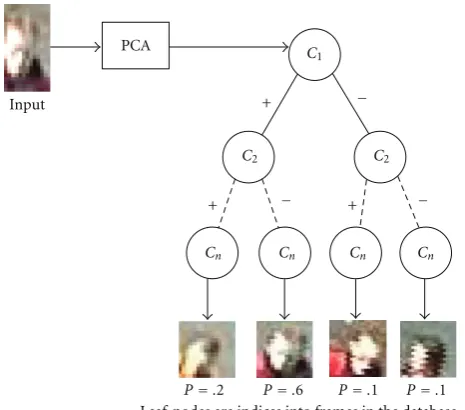
Figure 4: We sample from the exemplar databases to produce a
distribution over the training data given some input descriptor. In this case, the descriptor is the probability of skin/nonskin pixels in the face image shown at the top left. The PCA decomposition of the descriptor is used to decide how to traverse the binary tree, branching depending on the sign once the median has been subtracted (to balance the tree). At each branching of the tree a randomness factor is computed (based on a Gaussian) which results in the leaf nodes of the tree being explored. The leaf nodes are indices into the database which, in turn, point to specific frames in a sequence. We show here the illustrative matches generated for 10 samples with associated probabilities.
causal reasoning, this action-recognition system populates a set of “facts” which collects all the information available to the reasoning engine. This lower-level component of the system answers questions in a probabilistic fashion such as Where is the agent? What is he/she doing? Where are they looking? The language used ultimately to describe interactions is also defined at this stage by the expert’s hand-labelled descriptions of the exemplar data.
3.1. Visual Tracking. The extraction of low-level descriptions of activity is predicated on repeatedly locating a person in the video. Throughout this work we use the mean-shift tracker. The target of interest is initiated using background subtraction and the target model (histogram) thus defined. The mean-shift algorithm uses the Bhattacharyya coefficient as the similarity measure between two distributions which are discretised intoubins:p(y) at the current image window centred atyandq, the target model histogram. This is given by
ρp,q=
u
puqu, (1)
which is maximised for every frame using an efficient itera-tive algorithm [26]. We further employ occlusion reasoning to recover the track when a person disappears behind a tree or another person, for example. When the Bhattacharyya coefficient drops below a certain value, the search window is expanded by computing the Bhattacharyya coefficient for a grid of windows around the current location and, provided the target has not disappeared altogether or moved out with even this wider search region, the location can be recovered [27].
3.2. Gaze Direction Approximation. The first lower-level component of our system estimates where a person is looking in images where the head is typically in the range 20 to 40 pixels high [11]. In order to achieve head-pose estimation we use a feature vector based on skin detection to estimate the orientation of the head, which is discretised into 8 different orientations, relative to the camera. The pixels of the currently tracked head are compared to a reference skin histogram and weighted according to the likelihood that they are drawn from the same distribution. The visual tracker extracts a window containing the person in every frame. For accurate head-pose estimation we must centre the head within the window. As shown inFigure 1, automatic location of the head is achieved by segmenting the target using background subtraction and morphological operations with a kernel biased towards the scale of the target to identify objects. The head is taken as the top 1/7th of the entire body. The head is automatically centred in the bounding box at each time step to stabilise the tracking and provide an invariant descriptor for head pose. The descriptor of head pose is comprised of skin and nonskin pixels, which enables us to estimate 8 distinct head poses, as shown in
Figure 2. A fast sampling method returns a distribution
Frame 101 Frame 4 Frame 23
Frame 163
(a)
Gaze estimate angular error (degrees) 140
120 100 80 60 40 20 0
−20
−40
Er
ro
r
(deg
rees)
0 20 40 60 80 100 120 140 160 180 Frame
(b)
Figure5: Applying head-pose approximation to an urban scene. Error versus hand-labelled ground truth is shown on the right.
Optic-flow
(a)
Channels
Fbx+ Fbx−
Fby+ Fby−
6 5 4 3 2 1
1.2 1 0.8 0.6 0.4 0.2 0
8 6 4 2
8 6 4 2 0
×10−4
×10−4 ×10−4
×10−3
(b)
Figure6: The target-centred spatiotemporal action descriptor. (a) The optical flow vectors, (b) the blurred optic flow in thexandydirection is further split into the four Gaussian blurred nonnegative channels.
3.2.1. Fast Sampling from a Database of Labelled Exemplars.
Sidenbladh and Black structure a large database of high-dimensional points as a binary tree via principal component analysis of the data set [28]. The children of each node at level i in the tree are divided into two sets: those whose ith component (relative to the PCA basis) is larger and those whose value is smaller than the mean. In Sidenbladh’s application each data point comprised the concatenated joint angles over several frames of human motion capture data. The method, however, applies equally well to our application of image feature data and the pseudorandom search algorithm is identical to that derived in [28].
If Ψ is a length dmvector representing the median of all the sequences of head-pose descriptors (the skin/nonskin feature vectors), that is,
Ψ=1 n
n
i=1 Ψi,
A=Ψi,. . .,Ψn
(2)
Input frame
ML match
Best matching frame per sample Walk-LR
Walk-LR Walk-RL Walk-RL Walk-RL Walk-RL
Walk-RL
Walk-RL Walk-away Walk-away
Figure7: Pseudoprobabilistic sampling from the exemplar database. The input frame (top left) is shown beside the ML frame from 10 samples of the motion-descriptor database (top right). The more complete information is provided by the sampled distribution of matches from the database (bottom row).
Input frame
(a)
Database matches
Correct Correct Incorrect
Position Velocity Motion
(b)
Distribution over all actions
Walk-nearside-pavement Run-nearside-pavement
0.7 0.6 0.5 0.4 0.3 0.2 0.1 0
1 2 3 4 5 6 7 8 9 10 11 12 13 Model index
A
ct
ion
mo
del
p
ro
bs
P.V.M P.M
(c)
Frame Activity Likelihood Walking on far-side pavement
Walking on road
0.86 0.94 0.94
P1: walk fs pave P1: walk road P1: walk ns pave
1–70 71–225
226–450 Walking on nearside pavement
Figure9: An accurate commentary is obtained for this urban street scene where the person moving in from the top right of the images is under observation.
Frame 5336 Frame 5381 Frame 5462 Person jogging across road
Frames Estimated activity Road, running 5330–5470
Figure10: A second example of commentary extraction from a more challenging surveillance scene.
subtracted, by applying Singular Value Decomposition we write
A=UΣVT, (3)
where thedm×nmatrixUcontains the principal compo-nents ofAandΣis diagonal matrix containing the standard deviationσlaccounted for by the principal componentsl=
1,. . .,n. Any sequence in the database can be approximated by
Ψmatch=Ψ+Ucmatch, (4)
wherecmatch is the sampled nearest-neighbour match from one traversal of the binary tree.
Significantly, the first b = log2(n) (where n is the number of time intervals in the training data) components are selected.
If n ≈ 50000 and b = 16this accounts for 89%of the variance in the training data, that is,
b l=1σl2 n l=1σl2
≥0.89. (5)
These components are then organised into a binary tree; the nodes of which are split on the basis of the sign of the components once the median value has been subtracted:
ci=
ci,1,. . .,ci,b
. (6)
The search of the tree is randomised by the inclusion of a random perturbation of the traversal of the tree drawn from a Gaussian distribution. That is, it is decided which branch of the tree to choose, at each levellfor the Principal Component coefficient at that nodect,land the input coefficients at that
level,ci,l, based on the probabilities:
pright=p
ct,l≥0|ci,l
=√1
2πσl
ct,l
z=−∞exp −z2/2σ2
ldz,
pleft=1−pright.
(7)
(a) (b) (c)
0
−0.5
−1
−1.5
−2
−2.5
0 10 20 30 40 50 60 70 80 90
×104
Log
lik
Iteration
Cross-road Behaviour model logliks
Turn-into-drive Walk-along-near-side
(d)
Figure11: For the single person tracked (from top of image) in this video sequence we compute the likelihood of each of the behaviour models in the bank of models explaining the current action sequence. “Crossroad” is chosen as the correct model.
computed on the basis of how “close” the match in the database is to the input, that is,
pmatch|input∝exp− match−input σ
2 . (8)
This search method is used for two reasons: it is more efficient, and the ability to return multiple neighbours represents a distribution over possible actions, that is, a likelihood. The search time is improved by a factor of 20 and, since we sample many times, the search provides a set of particles which represents a distribution over the exemplar feature vectors into frames of the previously seen examples. An example of the distribution of frames at the nodes for a certain depth of the tree is given inFigure 3. An example of the sampling of previously seen examples from the tree is shown inFigure 4.
3.2.2. Combining Head Pose and Body Direction. The sam-pling method returns a distribution over possible head poses. Used on its own this can be noisy and so we use body direction to smooth the gazing approximation. Note that a number of assumptions are required which are
valid in large-scale outdoor surveillance scenes but may not hold in indoor situations or even different social settings (see [29]). These are, briefly, that the person does not change direction based on gaze, that anatomicallyimpossible gazes (looking backwards) are rejected and that gaze varies smoothly.
The overall body pose relative to the camera frame is approximated using the velocity of the body, obtained via automaticallyinitiated colour-based tracking in the image sequence. By combining direction and head-pose informa-tion gaze is determined more robustly than using each feature alone.
We compute the joint posterior distribution over direc-tion of modirec-tion and head pose, which gives us the gaze. The priors on these are initially uniform for direction of motion, reflecting the fact that there is no preference for any particular direction in the scene. For head pose however a centred, weighted function models a strong preference for looking forwards rather than sideways. The prior on gaze is defined specified using physical constraints, that is, by considering only physically possible gazes.
Walk in drive, turn-into-drive
(a)
Walk in drive, turn-into-drive
(b)
Figure12: A single HMM associated with theturning-into-drive behaviour is used to classify the same behaviour but performed in different ways. This is because the input/output to the stochastic model is distributions over instantaneous, abstracted actions, not image coordinates.
Gis the true gaze direction, andBis the true body direction, with all quantities referred to the ground centre. We then compute the joint probability of true body pose and true gaze:
P(B,G|d,h)∝P(d,h|B,G)P(B,G). (9)
Now given that the measurement of direction d is independent of both true gaze and measured head-poseG,h once true body Bpose is known, P(d | B,G,h) = P(d | B) and similarly that the measurement of head-pose h is independent of true body poseB given true gazeG,P(h | B,G)=p(h|G), then we have
P(B,G|d,h)∝P(h|G)P(d|B)P(G|B)P(B). (10)
We assume that the measurement errors in gaze and direction are unbiased and normally distributed around the respective true values
P(h|G)=NG,σG2
, P(d|B)=NB,σB2
. (11)
The joint prior, P(B,G) is factored as above intoP(G | B)P(B) where the first term encodes our knowledge that people tend to look straight ahead. Thus the distribution P(G | B) is peaked around B, while P(B) is taken to be uniform. This encodes our belief that all directions of body pose are equally likely.
Table1: Comparison of detection rate for three types of head-pose matching search.
Search type Accuracy (%) Time (secs)
NN (full data) 83.2 0.461
NN (PC coeffs) 81.9 0.426
Sampling 77.9 0.023
While for single frame estimation this formulation fuses the measurements (of head pose and body direction) with prior beliefs, when analysing video data we can further impose smoothness constraints to encode temporal coher-ence: the joint prior at time t is in this case taken to be P(Gt,Bt | Gt−1,Bt−1) = P(Gt | Bt,Gt−1)P(Bt | Bt−1), where we use the assumption that the current direction is independent of previous gaze. This is motivated by the observation that, in outdoor areas, people tend to have a fixed idea of where to go and this only changes due to major distractions in the visual field. We do recognise that, in a very limited set of cases (primarily indoors), this may in fact be a poor assumption since people may change their motion or pose in response to observing something interesting while gazing around. We also assume that current gaze depends only on current pose and previous gaze which is clearly a robust assumption. The former term, P(Gt | Bt,Gt−1), strikes a balance between the belief that people tend to look where they are going, and temporal consistency of gaze via a mixtureGt∼αN(Gt−1,σG2) + (1−α)N(Bt,σB2).
Now we compute the joint distribution for all 64 possible gazes resulting from possible combinations of 8 head poses and 8 directions. The discretisation of the full 360◦ into 8 poses is shown inFigure 2. This posterior distribution allows us to maintain probabilistic estimates without committing to a defined gaze, and this is advantageous for further reasoning about overall scene behaviour. Immediately though we can see that gazes which we consider very unlikely given our prior knowledge of human biomechanics (since the head cannot turn beyond 90◦relative to the torso [30]) can be rejected in addition to the obvious benefit that the quality of lower-level match can be incorporated in a mathematically sound way.
3.2.3. Results. Table 1shows the performance increase using
this method over nearest-neighbour search. As expected full comparison of the input descriptor (first row) gives best results with comparison using the Principal Components giving similar results. The sampling method described in the text returns a distribution over possible matches and the figures quoted are for the frequency of ML match corresponding to a true match and when a match is found in the distribution. While detection rate is inferior the probabilistic information can be exploited and the search is considerably faster.
Results from a range of test sequences show that we achieve gaze direction approximation with a median error of 5.5◦ using this method against standard surveillance scenes (the CAVIAR dataset (http://groups.inf.ed.ac.uk/vision/
CAVIAR/)). When applied to faces from our own Dataset 2
Extract features
Together rule Check
for events Facts
Event observed
Generate hypotheses and search facts while still data
Trigger events
Proximity rule
Meeting rule Cross-road
rule
Explanation Move-to-road
Cross-road
Meeting
Search available evidence Input
video
Updateable facts Predefined
Process Internal state
Figure13: A schematic diagram of the reasoning process initiated when the event “move-to-road” is detected.
Figure14: The second scene is divided into regions and labelled by an analyst. The semantically-labelled regions, activities and directions for this scene are detailed.
the median 0.5◦, as shown inFigure 5. The ground truth for this error computation is acquired by a human drawing an estimate of the line of sight of the person on the image. (We assume that this can be achieved to an accuracy of 10◦.) The error is therefore the difference between the approximated value and the quantised ground truth.
3.3. Spatiotemporal Action Recognition. In addition to gaze direction we also require to extract basic information about the position, velocity, and activity type (e.g., walking versus running versus standing) of an imaged person. We employ the same technique for sampling from hand-labelled exemplar databases as used for gaze direction approximation,
Figure 15: A subset of the trajectories in the exemplar data
representative of expected activity in this urban scene are shown here.
returning a probability distribution over a set of training examples, where the qualitative labels of place, direction, and action type have been identified by an expert user. This labelling holds three significant advantages:
(1) high-level descriptions can be incorporated by a qualified expert;
(2) by sampling nonparametrically from the data, far less training data is required than is the case for standard, statistic-based learning techniques such as Hidden Markov Models (HMMs);
Frame 135
(a)
Frame 197
(b)
Frame 304
(c)
Frame 247
(d)
Figure16: (Clockwise from top left). The “meeting” rule is initiated in this case.
Frame 30
(a)
Frame 95
(b)
Frame 175
(c)
Frame 115
(d)
Explanation
Person 2 move-to-road to meet on nearside-pavement Person 2 move-to-pavement to get-off-road
(a)
Explanation
Person 1 move-to-road to avoid Person 2 on nearside-pavement Person 1 move-to-pavement to get-off-road
(b)
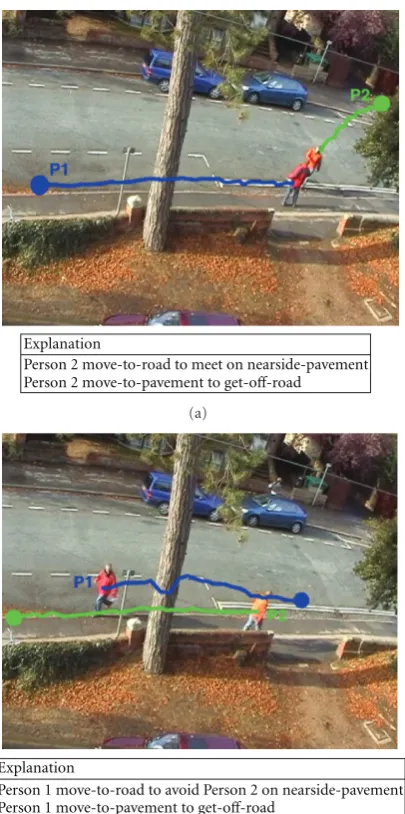
Figure 18: Causal explanations of interactions in an urban
scene. Meeting (left) and ignoring (right). By searching the action/behaviour/gaze, sensed by the agent of interest, for evidence of hypotheses generated in response to the automatically observed trigger event, the high-level explanations (below the frames, resp.) are automatically generated.
Position and velocity exemplars are derived directly from the centroid of the object as estimated using a colour-based tracker which fixates on the tracked person [26]. Action type is then encoded from the target-centred images using a descriptor based on optic flow, which is essentially the descriptor of Efros et al. [31]. This descriptor is derived from the flow vectors between image pairs. Four nonnegative channels are computed, as shown in Figure 6. These chan-nels provide sufficient discriminative power to differentiate among a set of basic actions when imaged at a distance.
The position, velocity, and action-type databases are maintained independently. This enables more efficient use of each feature, significantly reducing the overall volume of
training data required. The independent distributions over the feature databases are computed via an efficient Principal Components Analysis- (PCA-) based sampling tree. The output of one such sampling produces a discrete distribution as shown inFigure 7.
By fusing the likelihoods of the matches from the posi-tion, velocity, and motion-descriptor exemplars we compute the probability of a spatiotemporal actionsuch as walking-left-to-right-on-nearside-pavement. We use a Bayes Net to effect this information fusion: if the spatiotemporal action is denoted,a,xis the index into a qualitative position label in the database; similarly v is the index into a qualitative direction label, and m is the index into a person-centred action label, then assuming conditional independence yields
p(a,x,v,m)=p(a)p(x|a)p(v|a)p(m|a). (12)
The distributions p(xmatch | xinput), p(vmatch | vinput) and p(mmatch | minput) are estimated by sampling from the databases. We compute the marginal distributionp(a) since, for any given datad(herex,vandm),
p(d|a)= p(a|d)p(d)
p(a) . (13)
p(a | d) is specified in the conditional probability table for the nodea,p(d) is defined from the frequency of occurrence of datadin the training set andp(a) is uniform in most cases.
By taking the ML estimate from this distribution over all possible spatiotemporal actions at each time step, a com-mentary on activity is generated. An example of the MAP distribution which highlights the significance of each feature (position, motion-type, and velocity) is given inFigure 8. In this example, the ML motion type is incorrectly classified as
walking. When the resulting distributions from each of the inputs, position, velocity, and motion type are fused the ML estimate is now correctly identified as running-on-nearside-pavement. The action probability distributions when velocity is excluded (right-hand distribution) and included (left-hand distribution, i.e., shaded bars) are compared clearly showing the importance of each feature.
An example of the resulting commentary for surveillance video, which is achieved by taking the ML result at each frame, is shown in Figure 9. The priors on spatiotemporal actions are derived directly from the training datasets, on the basis of frequency of occurrence. They may also be specified by hand. In the second commentary example of
Figure 10, the priors are critical to the choice of the correct
spatiotemporal action. Running is not represented as often in the example database. Therefore if the priors for each simple action are computed on the basis of frequency, then the MAP spatiotemporal action for this sequence isroad, walking. If, however, the priors are uniform, the MAP result is as shown. Note that in either case the correct activity is still represented in the distribution over spatiotemporal actions.
Frame 646 Frame 468
Frame 437 Frame 380
Person crossing the road at traffic lights
Commentary on activity NE-pavement, walking N-ped-crossing, walking N-ped-crossing, stopped N-ped-crossing, walking NW-pavement, walking Explanation
Person move-to-road to cross-road at N-ped-crossing Person move-to-pavement to get-off-road
Figure19: The text commentary for a person crossing the road at a set of traffic lights provides the input to the reasoning engine. Here, there is no interaction between people, but domain knowledge allows the system to recognise that the person walked onto the road, in order to cross the road. The same rules and events set as used to generate the results inFigure 18is successfully used here in a different scene.
Commentary on activity Nearside pavement, walking Road, walking
Nearside pavement, walking
Explanation Inexplicable
Figure 20: (Clockwise from top left). This scenario is a failure mode for the system with the rule set defined in the text. For a causal reasoning system failure is an opportunity to learn. In this case a true anomaly has occurred, although in other circumstances this behaviour could be exhibited when a car is present, for example.
3.4. Behaviour as a Sequence of Spatiotemporal Actions.
Having successfully generated probability distributions over actions, we now use HMMs to encode known rules about behaviour. We define behaviour as spatiotemporal action extended over time. The MAP spatiotemporal action is an abstraction from the images to a description of activity in the scene in general. Taken on its own it provides a commentary on observed activity which is not dependent on one particular camera viewpoint. This enables us to derive an action sequence from an automatic
parse of extended behaviour. The hidden state of the HMM corresponds to a distribution over spatiotemporal actions. For the scene in Figure 11 we easily encoded 3 such HMM behaviour models (“crossing road”, “walking along pavement”, and “turning into drive”) by defin-ing the transition and initial-state probabilities for each model.
3.4.1. The Structure of the Behaviour HMM. The inputs to the HMM are two vectors containing the index into the spatiotemporal action and an associated probability of that action. The observation probabilities are discrete and the output of each state is the index into a spatiotemporal action (with associated likelihood). So, for example, for the behaviour “Crossroad”, above the parameters of the behaviour HMM are specified as follows:
Π= ⎛ ⎜ ⎜ ⎜ ⎜ ⎜ ⎜ ⎝ 1 0 0 0 ⎞ ⎟ ⎟ ⎟ ⎟ ⎟ ⎟ ⎠
, A=
⎛ ⎜ ⎜ ⎜ ⎜ ⎜ ⎜ ⎝
1 0 0 0
0 0.6 0.4 0
0.4 0 0.6 0
0 0 0 1
⎞ ⎟ ⎟ ⎟ ⎟ ⎟ ⎟ ⎠
, B=
⎛ ⎜ ⎜ ⎜ ⎜ ⎜ ⎜ ⎝
1 0 0 0
0 1 0 0
0 0 1 0
0 0 0 1 ⎞ ⎟ ⎟ ⎟ ⎟ ⎟ ⎟ ⎠ , (14)
where Π is the matrix of priors, A is the state transition matrix, andBis the observation matrix. The outputs from each state are parameterised by a Gaussian distribution centred on the state value. The states in this example correspond to
(1) walk on the nearside pavement, (2) walk on the far-side pavement, (3) walk on the road,
(4) walk in the driveway.
In the above example, the interpretation of the state transition matrix,Ais as follows.
(ii) When walking on the far-side pavement, the person will most likely keep walking on the far-side pave-ment (state 2), but a transition to the road (state 3) is allowed.
(iii) When walking on the road, the person will most likely stay walking on the road (state 3), but can move to the action walking on the nearside pavement (state 1). (iv) When the person is walking in the drive (state 4), no
transitions are allowed as this action is not expected to occur.
Similarly, behaviour HMMs are specified for the other behaviours, “Walking-along-nearside-pavement” (which is quite trivial, being a continuous sequence of walking-on-pavement actions) and “Turn-into-drive”.
3.4.2. Model Selection. Online estimation of which model best explains the observed MAP action sequence (not the raw image data) enables the estimation of higher-level behaviour. The ML sequence of actions and their likelihoods over a number of time steps is used to find the most likely behaviour by computing the likelihoods of each of the predefined normal behaviour HMMs explaining the current action sequence. Since more complex models generally explain data better we use a likelihood ratio to compare competing behaviour models. The likelihood ratio for comparing two hypotheses H and H with probabilities p(H) and p(H ), respectively, is computed as
LR=2logp(H)−logp(H), (15)
which has a chi-squared distribution parameterised by the difference in the model order. IfLRis greater than the 95% confidence value of the chi-squared distribution for δ = |O(H)−O(H )|, the result is statistically significant.
Note that a learning technique trained directly from the image data would require separate exemplars, multi-plying the training data volume. However since our HMM behaviour models are general to the scene they can dis-criminate between the same type of behaviour performed in different ways without the need for separate models. An example of this feature in operation is shown inFigure 12. When this technique is used to generate a smoothing prior on the action sequence we may achieve a significant improvement in action recognition (from 60% to 88%).
4. Reasoning about Interactions
Before describing in detail the causal reasoning process and its application in two specific example datasets we define the terminology used in the rest of this work. In particular, we explain the meaning of “events”, “rules”, and “facts”.
4.1. Explanation of Terminology: “Events”, “Rules” and “Facts”.
Our process for causal reasoning is to first specify a set of “events” and “rules” pertaining to the scene. When an event is observed by a single agent a search through the available evidencewhich is observable by that agentis performed. This
search seeks to explain the current known activity given the predefined rules. The low-level sensing component of the system abstracts the visual information into (ML) text descriptions of activity, the “rules” and “events” can be encoded simply as high-level conditional statements which act on the information available to the sensors of the agent. It should be noted that, while the full MAP distributions are available, only the ML text description is used by the reasoning system. A fully probabilistic reasoning process is much more ambitious and the subject of current work. A number of the rules are given in the appendix. An “event” is simply an occurrence which is predefined as interesting and requiring explanation, such as “cross-the-road”.
The events and the rules are changed between scenarios but the reasoning process remains the same. This reasoning process is given in pseudocode in Algorithm 1. Although we do specify the events which require explanation, this is not strictly necessary. One could mandate that it is only unexpected events that initiate the reasoning engine (where “unusual” is defined by some probability threshold on observed activity). Given that unusual activity is not modelled explicitly reasoning about such events requires a more sophisticated system than that which we develop here. We discuss how these might be handled by a rule-based reasoning system in Section 5.3.3. Hence, we specify the events which need explanation and these are preloaded into the system, along with the rules which govern the scene.
The final piece of information required is a set of “facts” on which the reasoning process operates, searching for an explanation given the “rules” and the “events”. The facts are gathered from the low-level sensing procedures as the video is processed and take the form of text descriptions of what is observed. These facts can be augmented with higher-level descriptions which have come from an earlier reasoning process. Thus the set of “facts” contains all the information which is available to the reasoning engine at any given time.
When a trigger event occurs, a search through the rules will take place. This is what we term generating a “hypothesis”, that is, postulating that one of the rules is in play. If any of the current facts lend evidence to any rule, the facts are updated. At the end of the video, the set of facts constitutes an “explanation”. We show this in operation in the following sections.
(1) load events-list (2) load rules
(3) check facts for event in events-list (4)forall frames in sequencedo (5) update facts list
(6) ifevent occursthen
(7) derive hypotheses from the rule-set (8) forall hypothesesdo
(9) search known facts for hypothesis support (10) end for
(11) end if (12)end for
Algorithm1: Reasoning process.
the “meeting” event, which is shown in Algorithm 4. A graphical illustration of this process for the “move-to-road” event is shown in the schematic,Figure 13.
4.3. Explaining Two-Person Interactions in an Urban Location.
The primary focus of this work is mutual interactions among people in urban surveillance. The predefined events and rules for reasoning about interactions in an urban context are listed inTable 2. We make the following assumptions about the agent.
(1) The agent has knowledge of his own state which includes action, behaviour, and gaze direction.
(2) The agent can see other agents when they fall within the visual field, determined by the gaze direction.
(3) The agent can sense anything within a specified range (reflecting the ability to, e.g., hear someone walking behind).
(4) Interactions between agents are possible within a certain proximity.
In the analysis of activity which follows it is important to note that there is no all-knowing reasoning process which has access to all the information taking place in the scene. The only information which is available is derived from the sensors of the agent of interest, that is, the agent whose behaviour corresponds to an activity which requires to be explained. As previously stated, this explicitly shifts the focus from the camera to the agent in the scene and thus reasons from the agent’s, as opposed to the global, view.
4.3.1. Detecting and Classifying Activities Using Rules. The true reasons for events occurring are not apparent directly from the video. A person who crossed the road in order to meet his friend may have done so because it was prearranged or because he happened to see his acquaintance. It is not possible to distinguish between these hypothetical reasons from the data alone even if the scene rules are completely known. Rather, it requires detailed knowledge of the intention, goals, and history of a specific individual. This is not generally available and certainly not in a surveillance
Table 2: The set of events which trigger the reasoning engine (left) and the set of rules which can be initiated in search of an explanation (right) are shown here.
Trigger events list Rules list
Move to road Potential meeting
Move to pavement Meeting
Move to drive Ignoring
Stopped Avoiding
Together Proximity
application where the individuals under observation are anonymous. Despite this fact, a “lower” level of causality is still in operation and this can be inferred from our description of the scenario: the person, “. . .crossed the road
in order to meet. . .”. This type of causality is amenable to analysis using the information we can currently obtain from the sensors of the agents.
People meeting with one another is a common occur-rence in an urban scene. In fact, recognising groups of people versus independent individuals and, in particular, detecting cooperating individuals, is a core element of the human interpretation of urban scenes. Police surveillance officers, for example, may be interested in an exchange of illegal substances at a meeting of two individuals under observation.
There are many cues humans use to distinguish between people meeting or people ignoring one another. One such cue, discussed inSection 3.2, is that people who are together will generally acknowledge each other’s presence bylooking
at one another periodically and at regular intervals. Other, more obvious cues include proximity. By defining precisely what is required for the event “meeting” to take place we can distinguish between people passing by one another and people meeting together.
The “proximity” of the individuals is first analysed using
Algorithm 2. A “potential meeting” is identified when agents
are within a predefined proximity in image coordinates for a predefined period of time (typically 100 frames) and also within one another’s field of view, that is, they must be looking at one another. Note that the value of proximity is preset in Algorithm 3. The number which ought to be chosen is dependent on many factors including social criteria and cultural norms [29] and is easily changed. The rule for meeting is that the intermediate state potential meeting must be the current explanation of the interaction. Additionally, the agents must be performing the same spatiotemporal action, for example, they are bothwalking-on-the-pavement. By contrast, an “ignore” rule is initiated when the conditions for “meeting” are not met but when a “potential meeting” has previously occurred. If none of these agent states are identified, there is no interaction defined.
algorithm explicitly requires input from the gaze direction approximation component of the system.
4.3.2. Explaining Interactions between People. There are a number of events which can be explained in terms of causal relations in a typical urban street scene. We assume that transitions in qualitative action generate interesting activity. These transitions are detailed in Table 2. The facts are therefore searched for evidence to support the particular hypotheses which may explain the event sequence (which have been generated in response to a predefined trigger event). For example, the transition between the actions
walking-on-far-side-pavementandwalking-on-roadgenerates an event “move-to-road”. Hypotheses for this particular scenario are defined as follows.
(1) IF the event “move-to-road” is followed by event “move-to-pavement” AND the current location is not the same as the location triggering the first event (i.e., the road is crossed) AND, subsequently, a meeting takes place THEN the explanation is that, “the agent crossed the road to meet the other agent”.
(2) IF a crossing of the road is observed NOT followed by an interaction THEN the explanation is that the agent crossed the road.
(3) IF a “move-to-road” event is triggered AND subse-quently a “move-to-pavement” event but back to the same pavement THEN no explanation is provided UNLESS another agent was in the near vicinity THEN the explanation is that it was necessary to avoid collision.
The pseudocode for this scenario is shown inAlgorithm 4 in the appendix. An illustrative schematic of the overall reasoning process for answering this question is shown in
Figure 13. Similarly, we generate hypotheses to explain events
including “stopping”, pavement” and “move-to-driveway”. It is simple to change between domains by updating the rule set. There is the additional advantage that the rule set is general to all such urban scenes. The output for two different situations is automatically generated and exactly the same reasoning engine and events set may be applied to each scene independently.
5. Experiments
Comprehensive data from two different urban scenes was gathered and used to evaluate our method. We first describe the datasets used and the training process, then discuss the evaluation of the reasoning process.
5.1. Dataset 1. The first dataset is illustrated inFigure 18. To obtain the data, two students were asked to act out a set of twelve two- and one-person activities. The activity was recorded using a standard home video camera from the second floor of a domestic building in Oxford. No instruction was given to the “actors”, other than a brief outline of the activity. The two-person activities included
walking together, meeting, passing one another by. A set of images containing these two-person activities was then extracted for experimentation. This subset of the total dataset comprises 6000 frames at 5 frames per second (fps). From this, a hand-labelled corpus of 665 frames was generated by the authors for training the low-level sensing component of the system. The low-level spatiotemporal action classes derived from these sequences are walking (away, towards, left, and right), running (away, towards, left, and right), and standing still. The people are tracked automatically and the representative (training) action classes are labelled by hand. The head-pose classes remain as described previously and database exemplars of the head-pose under these imaging conditions were extracted automatically and then given a semantic label by hand. The positional locations are defined as nearside pavement, far-side pavement, road, and driveway.
5.2. Dataset 2. For the second scene shown in Figure 14 no actors were used. People are imaged in this dataset performing normal activity such as crossing the road, walking together on the pavement. This data was acquired from the roof of the IEB building at Oxford University. A total of 76,040 frames at 5 fps was recorded and a training set of 4491 frames created corresponding to interesting activity extracted from the overall data. The low-level action classes are labelled as walking, running, and standing. Position locations are defined as shown in the hand segmented scene in Figure 14. The positional labels are, for example, Northbound Lane (3), Right Turn Lane (4), Southbound Lane (6), Parks Road Westbound (7), and so forth. These, taken with the semantic labels of the actions determine the human-readable output used to generate readable text descriptions.
A database of action exemplars was collected from training examples. Some of the training trajectories are shown inFigure 15. Once more, the head-pose exemplars are extracted from the dataset. The training phase and semantic labelling for a new dataset such as this takes less than 30 minutes and was performed by one person—a researcher— who is familiar with the area, hence the descriptive semantic labels of positional areas.
5.3. Results
5.3.2. Explanations of Events. The interpretation of the events is dependent on the detection of lower-level events. The explanatory hypotheses have already been discussed in some detail inSection 4.3. Out of the data used in this paper we identified the four events in Dataset 1 which are already listed
in Table 2. In Dataset 2 this set is augmented by a series
of single-person interactions with the environment. Given the “real” nature of this particular dataset, the events are somewhat uninteresting and correspond to road crossings mainly.
Over both datasets, using the spatiotemporal actions and gaze estimator as inputs to the higher-level rule set, we find that the system derives a correct explanation on 79% of the occasions in which a human observer identifies an event has occurred. This is the mean recognition rate in both sequences. Note that failure at the low-level sensing stage has a critical impact on this statistic. As such, we could not improve the mean 88% recognition rate of the action/behaviour/gaze estimate. Meeting and ignoring events are successfully recognised and examples of these events are Figures16and 17. This enables the facts list to be updated and for explanations to be generated. To validate the method we focus on explanations of “crossing the road” events for the reason that this event is common in both of our test datasets. This enable us to reach a variety of explanations and also to test the extensibility of the rule-based approach. The results presented in Figures18 and 19show the success of the technique. In Dataset 1 two different scenarios unfold and both scenarios result in a plausible human-readable explanation of the activity. In the first case the “meeting” is given as the reason for the event, in the second, “avoid” is given (seeFigure 18).
The result drawn from Dataset 2 shows how the rea-soning process may be extended. In this case there is no other person and so a new explanation is posited: that of “crossing road”. The rules are augmented for the example
inFigure 19with knowledge that the road may legitimately
be crossed at the pedestrian crossing, that is, despite there being no evidence for a meeting, crossing at the lights is a plausible reason for the observed behaviour. The accuracy of the method is demonstrated here also by the running commentary generated inFigure 19.
5.3.3. Failure Modes. The role of learning in a causal reasoning system is significant. We recognise that failure of any current implementation for a given scenario is either (a) an opportunity to learn, or (b) an opportunity to identify unusual/inexplicable behaviour. The latter may be used to prompt a surveillance analyst. Otherwise, when no conclusion can be reached, the user can be prompted to update the rule set to encompass the scenario encountered. An example of an inexplicable event for the system presented in this paper is shown in Figure 20, where a person is observed to walk on one pavement, the road, and then return to the same pavement. Given the rule set defined in the appendix, no explanation can be derived. It can be seen that this behaviour is genuinely inexplicable. However, were a car driving along the road, an appropriate rule fix might
(1) load facts
(2) proximityThreshold=100 (3) timeThreshold=100 (4)forall framesdo
(5) distance=(P1 position)−(P2 position) (6) ifdistance≤proximityThresholdthen
(7) ifp1action=p2action & P1 visible & P2 visible then
(8) together=1
(9) increment=increment + 1 (10) end if
(11) end if
(12) if increment≥timeThreshthen (13) situation=“together” (14) else
(15) situation=“not together” (16) end if
(17) update facts (18)end for
Algorithm2: Proximity rule.
(1) load facts
(2) meetingThresh=50 (3) j=lastFrameIndex (4)fori=1 tojdo
(5) ifsituation(i)=situation(i−1)then (6) ifsituation(i)=“together”then (7) togetherInc=togetherInc + 1 (8) else
(9) togetherInc=0 (10) end if
(11) end if
(12) iftogetherInc≥meetingThreshthen (13) scenario=“meeting”
(14) else iftogetherInc<meetingThresh & togetherInc>0 Then
(15) scenario=“potential meeting” (16) else
(17) scenario=“not meeting” (18) end if
(19) update facts (20)end for
Algorithm3: Meeting rule.
include knowledge of a pedestrian’s desire to avoid traffic. This augmentation of the rule set would result in a plausible interpretation of activity.
6. Conclusion
(1) load facts
(2)ifevent=“meeting”then (3) for j=1 to lastFramedo (4) ifscenario=“meeting”then
(5) currentAction=facts·positionLabel(j) (6) explanation=“Person” event “to meet on”
currentAction (7) end if
(8) end for
(9) for j=1 to lastFramedo (10) if scenario=“ignore”then
(11) currentAction=facts·positionLabel(j) (12) explanation=“Person” event “to avoid other
Person on” currentAction (13) end if
(14) end for (15)end if
Algorithm4: Move-to-road rule.
recognition, the results of which we have exploited to enable a software “agent” to sense its environment. Using known rules about how agents interact, we created a general method for reasoning about causal interactions between people. The generality of the method is clearly demonstrated by the results from two very different applications. The most pressing area for future work is to implement a fully Bayesian reasoning system.
Appendix
See Algorithms2,3, and4.
Acknowledgment
Neil Robertson was supported by the Royal Commission for the Exhibition of 1851 and the UK Ministry of Defence.
References
[1] R. Gerber, H. Nagel, and H. Schreiber, “Deriving textual descriptions of road traffic queues from video sequences,” in Proceedings of European Conference on Artifical Intelligence, pp. 736–740, 2002.
[2] M. Brand, L. Birnbaum, and P. Cooper, “Sensible scenes: visual understanding of complex structures through causal analysis,” inProceedings of National Conference on Artificial Intelligence, Washington, DC, USA, 1993.
[3] A. Michotte,The Perception of Causality, Basic Books, 1946, English translation, Methuen, Andover, Mass, USA, 1963. [4] F. Heider and M. Simmel, “An experimental study of apparent
behaviour,”American Journal of Psychology, vol. 57, pp. 243– 249, 1944.
[5] B. J. Scholl, “Innateness and (Bayesian) visual perception,” in The Innate Mind: Structure and Contents, P. Carruthers, S. Laurence, and S. Stich, Eds., pp. 34–52, Oxford University Press, Oxford, UK, 2005.
[6] P. R. Cooper and M. A. Brand, “A knowledge framework for seeing and learning,” inVisual Learning, Volume 2: Symbolic Visual Learning, K. Ikeuchi and M. Veloso, Eds., Oxford University Press, Oxford, UK, 1995.
[7] J. Pearl,Causality. Models, Reasoning and Inference, Cambridge University Press, Cambridge, UK, 2000.
[8] M. Rigolli, Q. Williams, M. J. Gooding, and M. Brady, “Driver behavioural classification from trajectory data,” inProceedings of the 8th International IEEE Conference on Intelligent Trans-portation Systems (ITSC ’05), pp. 889–894, Vienna, Austria, September 2005.
[9] J. M. Siskind, “Grounding the lexical semantics of verbs in visual perception using force dynamics and event logic,” Journal of Artificial Intelligence Research, vol. 15, pp. 31–90, 2001.
[10] N. Robertson and I. Reid, “Behaviour understanding in video: a combined method,” in Proceedings of the International Conference on Computer Vision (ICCV ’05), pp. 808–815, October 2005.
[11] N. Robertson and I. Reid, “Estimating gaze direction from low-resolution faces in video,” in Proceedings of the 9th European Conference on Computer Vision (ECCV ’06), vol. 3952 ofLecture Notes in Computer Science, pp. 402–415, Graz, Austria, May 2006.
[12] S. Russel and P. Norvig, Artificial Intelligence, A Modern Approach, Prentice-Hall, New York, NY, USA, 1995.
[13] E. L. Andrade and R. B. Fisher, “Simulation of crowd problems for computer vision,” inProceedings of the 1st International Workshop on Crowd Simulation (VCROWDS ’05), Lausanne, Switzerland, November 2005.
[14] M. E. Bratman,Intention, Plans, and Practical Reason, CSLI Publications, Stanford University, 1988.
[15] M. Georgeff, B. Pell, M. Pollack, M. Tambe, and M. Wooldridge, “The belief-desire-intention model of agency,” in Proceedings of the 5th International Workshop on Intelli-gent AIntelli-gents V : AIntelli-gent Theories, Architectures, and Languages (ATAL ’98), pp. 1–10, 1999.
[16] H. Dee and D. Hogg, “Detecting inexplicable behaviour,” in Proceedings of the British Machine Vision Conference, vol. 2, pp. 597–606, 2004.
[17] G. Medioni, I. Cohen, F. Br´emond, S. Hongeng, and R. Nevatia, “Event detection and analysis from video streams,” IEEE Transactions on Pattern Analysis and Machine Intelligence, vol. 23, no. 8, pp. 873–889, 2001.
[18] S. Gong and T. Xiang, “Recognition of group activities using dynamic probabilistic networks,” inProceedings of the 9th IEEE International Conference on Computer Vision, vol. 2, pp. 742– 749, IEEE Computer Society, Nice, France, October 2003. [19] N. T. Nguyen, D. Q. Phung, S. Venkatesh, and H. Bui,
“Learning and detecting activities from movement trajectories using the hierarchical hidden Markov model,” inProceedings of the IEEE Computer Society Conference on Computer Vision and Pattern Recognition (CVPR ’05), vol. 2, pp. 955–960, San Diego, Calif, USA, June 2005.
[20] S. Hongeng and R. Nevatia, “Large-scale event detection using semi-hidden Markov models,” inProceedings of the 9th IEEE International Conference on Computer Vision, vol. 2, pp. 1455– 1462, IEEE Computer Society, Nice, France, October 2003. [21] P. K. Turaga, A. Veeraraghavan, and R. Chellappa, “From
[22] J. J. Buckley,Fuzzy Expert Systems and Fuzzy Reasoning William Siler, 2005.
[23] M. Rigolli and D. Phil, thesis, Department of Engineering Science, University of Oxford, 2006.
[24] X. Liu, N. Krahnstoever, T. Yu, and P. Tu, “What are customers looking at?” inProceedings of IEEE Conference on Advanced Video and Signal Based Surveillance (AVSS ’07), pp. 405–410, September 2007.
[25] N. Robertson and I. Reid, “A general method for human activity recognition in video,” Computer Vision and Image Understanding, vol. 104, no. 2-3, pp. 232–248, 2006.
[26] D. Comaniciu and P. Meet, “Mean shift analysis and applica-tions,” inProceedings of the 7th IEEE International Conference on Computer Vision (ICCV ’99), vol. 2, pp. 1197–1203, September 1999.
[27] C. Bibby and I. Reid, “Visual tracking at sea,” inProceedings of the International Conference on Robotics and Applications, Barcelona, Spain, 2005.
[28] H. Sidenbladh, M. Black, and L. Sigal, “Implicit probabilistic models of human motion for synthesis and tracking,” in Proceedings of the European Conference on Computer Vision, vol. 1, pp. 784–800, June 2002.
[29] E. M. Rogers, W. B. Hart, and Y. Miike, “Edward T. Hall and the history of intercultural communication: the United States and Japan,”Keio Communication Review, vol. 24, pp. 3–26, 2002.
[30] D. Pang and V. Li, “Atlantoaxial rotatory fixation: part 1— biomechanics of normal rotation at the atlantoaxial joint in children,”Neurosurgery, vol. 55, no. 3, pp. 614–625, 2004. [31] A. A. Efros, A. C. Berg, G. Mori, and J. Malik, “Recognizing