The Use of Computational Thermodynamics to Predict Properties of Multicomponent Materials for Nuclear Applications

(1)

Centre

of

Excellence

for

Nuclear

Materials

Workshop

Materials

Innovation

for

Nuclear Optimized

Systems

December 5-7, 2012, CEA – INSTN Saclay, France

Bo SUNDMAN et al.

KTH (Sweden) and CEA-INSTN (France)

The Use of Computational Thermodynamics to Predict

Properties of Multicomponent Materials for Nuclear

Applications

Workshop

organized

by:

Christophe

GALLÉ,

CEA/MINOS,

Saclay

–

Constantin

MEIS,

CEA/INSTN,

Saclay

–

Workshop

Materials

Innovation

for

Nuclear

Optimized

Systems

December 5-7, 2012, CEA – INSTN Saclay, France

The Use of Computational Thermodynamics to Predict Properties of

Multicomponent Materials for Nuclear Applications

Bo SUNDMAN

1

, Christine GUÉNEAU

2

1_{KTH (Stockholm, Sweden), ISNTN (Saclay, France)}

2

CEA-DEN-DPC, Service de la Corrosion et du Comportement des Matériaux dans leur Environnement, SCCME (Saclay, France)

Computational Thermodynamics is based on physically realistic models to describe metallic and oxide crystalline phases as well as the liquid and the gas in a consistent manner [1]. The models are used to assess experimental and theoretical data for many different materials and several thermodynamic databases has been developed for steels, ceramics, semiconductor materials as well as materials for nuclear applications.

Within CEA a long term work is ongoing to develop a database for the properties of nuclear fuels and structural materials [2].

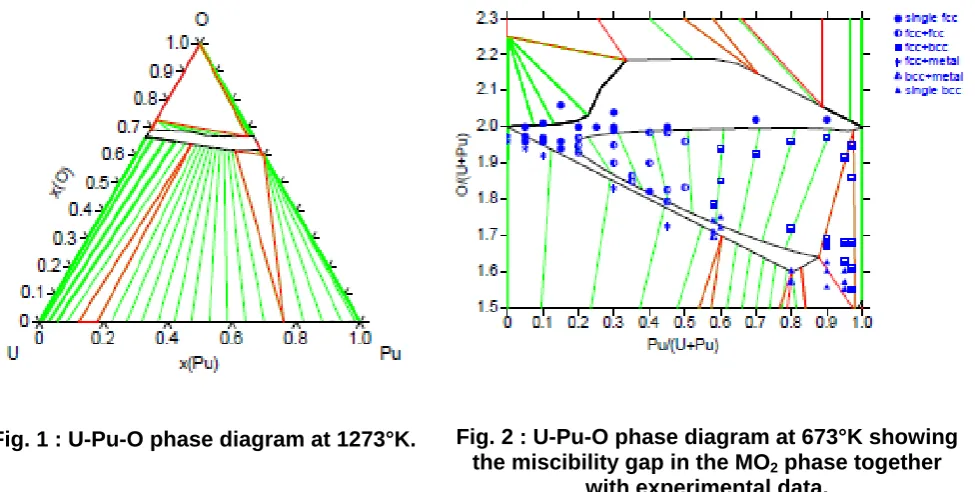
An overview of the modeling technique will be given and several examples of the application of the database to different problems, both for traditional phase diagram calculations and its use in simulating phase transformations. The following diagrams (Fig. 1, Fig. 2 and Fig.3) show calculations in the U-Pu-O system.

Fig. 1 : U-Pu-O phase diagram at 1273°K. Fig. 2 : U-Pu-O phase diagram at 673°K showing

the miscibility gap in the MO2 phase together

with experimental data. EPJ Web of Conferences 51, 01006 (2013)

DOI: 10.1051/epjconf/20135101006

(3)

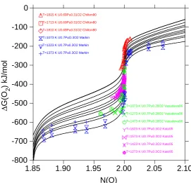
-800 -700 -600 -500 -400 -300 -200 -100 0 Δ G(O 2 ) kJ/mol

1.85 1.90 1.95 2.00 2.05 2.10

N(O) T=1815 K U0.69Pu0.31O2 Chilton80

T=1713 K U0.69Pu0.31O2 Chilton80

T=1810 K U0.69Pu0.31O2 Chilton80

T=1073 K U0.7PuO.3O2 Markin

T=1223 K U0.7Pu0.3O2 Markin

T=1373 K U0.7Pu0.3O2 Markin

T=1073 K U0.7Pu0.28O2 Vasudeva06

T=1623 K U0.7Pu0.3O2 Kato05

T=1573 K U0.7Pu0.3O2 Kato05

T=1423 K U0.7Pu0.3O2 Kato05

T=1273 K U0.7Pu0.3O2 Kato05

Fig. 3 : Oxygen chemical potentials at different temperatures and varying oxygen content for systems with Pu/u ratios around 0.3, together with experimantal data.

References

[1] H. Lukas, S. Fries, B. Sundman, Computational Thermodynamics. Cambridge University Press (2007).

[2] C. Guéneau, N. Dupin, B. Sundman, C. Martial, J.-C. Dumas, S. Gossé, S. Chatain, F. De Bruycker, D. Manar, R.J.M. Konings, Thermodynamic modeling of advanced oxide and carbide nuclear fuels: description of the U-Pu-O-C systems. J. Nucl Mater. 419 (2011) 145

Workshop

Materials

Innovation

for

Nuclear

Optimized

Systems

(4)

The use of Computational Thermodynamics to

predict properties of multicomponent materials

for nuclear applications

Bo Sundman and Christine Gu´eneau

INSTN and DEN/DANS/DPC/SCCME, CEA Saclay

(5)

Abstract

Computational Thermodynamics is based on physically realistic models to describe metallic and oxide crystalline phases as well as the liquid and gas in a consistent manner. The models are used to assess experimental and theoretical data for many different

materials and several thermodynamic databases has been

developed for steels, ceramics, semiconductor materials as well as materials for nuclear applications.

Within CEA a long term work is ongoing to develop a database for the properties of nuclear fuels and structural materials.

An overview of the modelling technique will be given and several examples of the application of the database to different problems.

(6)

Outline

◮ Thermodynamics

(7)

Outline

◮ Thermodynamics

◮ Computational Thermodynamics (CT, Calphad)

◮ models,

(8)

Outline

◮ Thermodynamics

◮ models, ◮ software

(9)

Outline

◮ Thermodynamics

◮ assessments and databases

(10)

Outline

◮ Thermodynamics

◮ The fuelbase database.

(11)

Outline

◮ Thermodynamics

◮ Modelling oxides.

(12)

Outline

◮ Thermodynamics

◮ Summary and conclusions

(13)

Outline

◮ Thermodynamics

◮ Summary and conclusions

Literature:

◮ Nigel Saunders and Peter Miodownik, Calphad, Pergamon

Materials Series, Vol 1 (1998)

◮ Mats Hillert: Phase Equilibria, Phase Diagrams and Phase

Transformations, 2nd edition, Cambridge (2008).

◮ Leo Lukas, Suzana Fries and Bo Sundman,Computational

Thermodynamics, Cambridge (2007).

(14)

Classical Thermodynamics

Thermodynamics is a phenomenological theory describing the

relation between some observable properties like temperature, T,

pressure, P, heat Q, etc.

(15)

Classical Thermodynamics

It is founded on two simple laws for macroscopic systems:

1. Energy cannot be destroyed or created,

(16)

Classical Thermodynamics

2. Heat never flows spontaneously from a cold body to a hot

body

(17)

Classical Thermodynamics

2. Heat never flows spontaneously from a cold body to a hot

body

These laws, and some trivial mathematics, makes it possible to

define a number of additional properties like internal energy, U,

entropy, S, Gibbs energy, G etc. These are not observables but can

be used to derive strict mathematical relations between many properties.

(18)

Properties derived from the Gibbs energy

S = −

∂G

∂T

P,Ni

H = G −TS V =

∂G

∂P

T,Ni

µi =

∂G

∂Ni

T,P,Nj6=i

(19)

Properties derived from the Gibbs energy

S = −

∂G

∂T

P,Ni

H = G −TS V =

∂G

∂P

T,Ni

µi =

∂G

∂Ni

T,P,Nj6=i

CP = −T

∂2G

∂T2

P,Ni

α = 1

V

∂2G

∂P∂T

Ni

κ = −1

V

∂2G

∂P2

T,Ni

(20)

Computational Thermodynamics: Central part of science

(21)

Computational Thermodynamics: Models 1

The Gibbs energy has been selected for modelling materials properties using the Calphad method. The main reason is that

most experimental data is known at constant T andP.

(22)

Computational Thermodynamics: Models 1

T andP are intensive properties and simple polynomials can be

used to describe theT and P dependence, but for very high

pressures special models are needed.

(23)

Computational Thermodynamics: Models 1

Modelling the composition dependence is the more complicated. There are two reasons for this:

◮ the amount of a component, N_i is an extensive property,

(24)

Computational Thermodynamics: Models 1

◮ the configurational entropy is very important.

(25)

Computational Thermodynamics: Models 1

◮ the configurational entropy is very important.

For the configurational entropy one must take into account the formation of molecules in a gas phase, crystalline sites in solids, charge transfer between elements, clusters etc. In many cases it is necessary to introduce more constituents of the phases than just the components.

(26)

Computational Thermodynamics: Models 2

Most materials consists of several crystalline phases with different structure and properties. The material often interact with other phases like gas and liquids.

The Gibbs energy is an extensive property and it is possible to model each phase separately:

G = X α

ℵα_Gα

m(T,P,yi)

whereℵα_{is the number of moles and}_Gα

m is the molar Gibbs energy

of of the phase α.

(27)

Computational Thermodynamics: Models 2

G = X α

ℵα_Gα

m(T,P,yi)

of of the phase α.The molar Gibbs energy is written as a function

of the constituent fractions, yi, to model the configuration of the

phase. In this way each phase can be modelled independently.

(28)

Computational Thermodynamics: Models 2

G = X α

ℵα_Gα

m(T,P,yi)

of of the phase α.The molar Gibbs energy is written as a function

of the constituent fractions, yi, to model the configuration of the

phase. In this way each phase can be modelled independently. The equilibrium is found by minimizing the total Gibbs energy for the given set of external conditions.

(29)

Computational Thermodynamics: Models 3

In a gas phase the molecules like H2, H2O, O2 etc. are the

constituents. The mole fraction of component i in the gas is

x_igas =

P

jbijyjgas P

k P

jbkjy_jgas

where bij is the stoichiometric ratio of component i in j.

(30)

Computational Thermodynamics: Models 3

In a gas phase the molecules like H2, H2O, O2 etc. are the

constituents. The mole fraction of component i in the gas is

x_igas =

P

jbijyjgas P

k P

jbkjy_jgas

where bij is the stoichiometric ratio of component i in j.

In a crystalline phase one may have several sublattices with are preferred by different elements.

xα

i = P

sasPjbijy_j(s),α P

sasPk P

jbkjyj(s),α

where as is the number of sites on sublattices, bij is the

stoichiometric factor and y_i(s) is the fraction of constituent i on

sublattice s.

(31)

Computational Thermodynamics: Models 4

The figures below represent three crystalline structures, B1, D8b

and D03 which require sublattices to be modelled.

The Compound Energy Formalism (CEF) assumes random mixing of the constituents on each sublattice which gives the

configurational entropy as

cfg_S

m = X

s

as X

i

y_i(s)ln(y_i(s))

(32)

Computational Thermodynamics: Models 5

The end member is an important concept in CEF defining one specific constituent in each sublattice. This defines a compound and the surface of reference for the phase:

srf_G

m= X

I Y

iI

y_i(s) ◦_G

I

where I has one constituent i in each subalttice s and ◦_G

I is the

Gibbs energy of formation of this compound from the reference

states of the elements, depending only on T andP.

(33)

Computational Thermodynamics: Models 5

The end member is an important concept in CEF defining one specific constituent in each sublattice. This defines a compound and the surface of reference for the phase:

srf_G

m= X

I Y

iI

y_i(s) ◦_G

I

where I has one constituent i in each subalttice s and ◦_G

I is the

Gibbs energy of formation of this compound from the reference

states of the elements, depending only on T andP.

In order to represent the interaction energy between the constituents in sublatticies there is an excess Gibbs energy:

E_G m=

X

J Y

jJ

y_j(s)LJ

where J has one or more constituents in each sublattice andLJ

describe the properties of real phases.

(34)

Computational Thermodynamics: Software 1

There are several commercial software for equilibrium calculations and they offer slightly different ways to control a system. The

simplest way is to specify T,P and the amount of all components.

(35)

Computational Thermodynamics: Software 1

But a user may prefer to specify the chemical potential, µi of a

component i or its activity or one or more of the stable phases or

maybe even the composition of a specific phase.

(36)

Computational Thermodynamics: Software 1

By varying one of the conditions one can calculate how the system

varies with this and that is known as aproperty diagram.

Oxygen potentials in UO2

-25 -20 -15 -10 -5 0 log10(pO 2 ) bar

1.8 1.9 2.0 2.1 2.2 O/U T=2700 K T=2600 K T=2500 K T=2400 K T=2300 K T=2250 K T=2200 K T=2100 K T=2000 K T=1950 K T=1900 K T=1800 K T=1700 K T=1600 K T=1500 K T=1400 K T=1300 K T=1200 K T=1100 K T=1000 K T=900 K T=800 K

(37)

Computational Thermodynamics: Software 1

-25 -20 -15 -10 -5 0 log10(pO 2 ) bar

The heat capacity of UO2

(38)

Computational Thermodynamics: Software 1

-25 -20 -15 -10 -5 0 log10(pO 2 ) bar

The heat capacity of UO2 Phase fractions in MOX

0 0.5 1.0 1.5 2.0 2.5 3.0

Amount of phase

0 500 1000 1500 2000 2500 3000 3500

T/K

(39)

Computational Thermodynamics: Software 2

When two or more conditions are allowed to vary the software will

calculate a phase diagramwhere the lines separate regions with

different sets of stable phases.

0 500 1000 1500 2000 2500 3000 3500 T/K

0 0.2 0.4 0.6 0.8 1.0 Mole fraction O

liquid C1

hcp bcc

O-Zr phase diagram

1.5 1.6 1.7 1.8 1.9 2.0 2.1 2.2 2.3 O/(U+Pu)

0 0.10.20.30.40.50.60.70.80.91.0 Pu/(U+Pu) single fcc fcc+fcc fcc+bcc fcc+metal bcc+metal single bcc

Isothermal section of O-Pu-U Isopleth of C-O-Pu-U

The leftmost diagram is the O-Zr phase diagram, the middle diagram is an isothermal section at 473 K of the O-Pu-U phase diagram and the rightmost an isopleth section of the C-O-Pu-U system.

(40)

Computational Thermodynamics: Software 3

The diagrams below show the modelled Gibbs energy functions for two phases in a binary system at 3 different temperatures.

-7 -6 -5 -4 -3 -2 -1 0 1 2

Gibbs energy J/mol

0 0.2 0.4 0.6 0.8 1.0 Mole fraction Cu

fcc liquid -3 -2 -1 0 1 2 3

Gibbs energy kJ/mol

0 0.2 0.4 0.6 0.8 1.0 Mole fraction Cu

fcc liquid -1.0 -0.5 0 0.5 1.0 1.5 2.0

Gibbs energy kJ/mol

0 0.2 0.4 0.6 0.8 1.0 Mole fraction Cu

liquid

fcc

(41)

Computational Thermodynamics: Software 3

-7 -6 -5 -4 -3 -2 -1 0 1 2

Gibbs energy J/mol

0 0.2 0.4 0.6 0.8 1.0 Mole fraction Cu

fcc liquid -3 -2 -1 0 1 2 3

Gibbs energy kJ/mol

0 0.2 0.4 0.6 0.8 1.0 Mole fraction Cu

fcc liquid -1.0 -0.5 0 0.5 1.0 1.5 2.0

Gibbs energy kJ/mol

0 0.2 0.4 0.6 0.8 1.0 Mole fraction Cu

liquid

fcc

The equilibrium state for any temperature and composition is the lowest Gibbs energy.

(42)

Computational Thermodynamics: Software 3

-7 -6 -5 -4 -3 -2 -1 0 1 2

Gibbs energy J/mol

0 0.2 0.4 0.6 0.8 1.0 Mole fraction Cu

fcc liquid -3 -2 -1 0 1 2 3

Gibbs energy kJ/mol

0 0.2 0.4 0.6 0.8 1.0 Mole fraction Cu

fcc liquid -1.0 -0.5 0 0.5 1.0 1.5 2.0

Gibbs energy kJ/mol

0 0.2 0.4 0.6 0.8 1.0 Mole fraction Cu

liquid

fcc

The equilibrium state for any temperature and composition is the lowest Gibbs energy.The end points to a tangent to a Gibbs energy curve gives the chemical potential of the components,

µi =

∂G

∂Ni

T,P,Nj6=i

(43)

Computational Thermodynamics: Software 3

-7 -6 -5 -4 -3 -2 -1 0 1 2

Gibbs energy J/mol

0 0.2 0.4 0.6 0.8 1.0 Mole fraction Cu

fcc liquid -3 -2 -1 0 1 2 3

Gibbs energy kJ/mol

0 0.2 0.4 0.6 0.8 1.0 Mole fraction Cu

fcc liquid -1.0 -0.5 0 0.5 1.0 1.5 2.0

Gibbs energy kJ/mol

0 0.2 0.4 0.6 0.8 1.0 Mole fraction Cu

liquid

fcc

The equilibrium state for any temperature and composition is the lowest Gibbs energy.The end points to a tangent to a Gibbs energy curve gives the chemical potential of the components,

µi =

∂G

∂Ni

T,P,Nj6=i

As the Gibbs energy curves are modelled outside the stable range of the phases it is possible to calculate metastable states.

(44)

Computational Thermodynamics: Software 3

-7 -6 -5 -4 -3 -2 -1 0 1 2

Gibbs energy J/mol

0 0.2 0.4 0.6 0.8 1.0 Mole fraction Cu

fcc liquid -3 -2 -1 0 1 2 3

Gibbs energy kJ/mol

0 0.2 0.4 0.6 0.8 1.0 Mole fraction Cu

fcc liquid -1.0 -0.5 0 0.5 1.0 1.5 2.0

Gibbs energy kJ/mol

0 0.2 0.4 0.6 0.8 1.0 Mole fraction Cu

liquid

fcc

In two-phase regions the common tangentsto the Gibbs energy

curves gives the most stable state.

The vertical dashed lines indicate the compositions of the phases for the common tangents.

(45)

Computational Thermodynamics: Software 3

-7 -6 -5 -4 -3 -2 -1 0 1 2

Gibbs energy J/mol

0 0.2 0.4 0.6 0.8 1.0 Mole fraction Cu

fcc liquid -3 -2 -1 0 1 2 3

Gibbs energy kJ/mol

0 0.2 0.4 0.6 0.8 1.0 Mole fraction Cu

fcc liquid -1.0 -0.5 0 0.5 1.0 1.5 2.0

Gibbs energy kJ/mol

0 0.2 0.4 0.6 0.8 1.0 Mole fraction Cu

liquid fcc 600 700 800 900 1000 1100 1200 1300 1400 T/K

0 0.2 0.4 0.6 0.8 1.0 Mole fraction Cu

liquid fcc fcc 600 700 800 900 1000 1100 1200 1300 1400 T/K

0 0.2 0.4 0.6 0.8 1.0 Mole fraction Cu

liquid fcc fcc 600 700 800 900 1000 1100 1200 1300 1400 T/K

0 0.2 0.4 0.6 0.8 1.0 Mole fraction Cu

liquid

fcc

The solubility lines in the phase diagram are obtained by joining the points of the common tangents at varying temperatures.

(46)

Computational Thermodynamics: Databases 1

In a CT database is stored:

◮ the model descriptions for each assessed phase,

(47)

Computational Thermodynamics: Databases 1

◮ the end member energies, ◦G

I,

(48)

Computational Thermodynamics: Databases 1

I,

◮ the interaction energies, L

J.

(49)

Computational Thermodynamics: Databases 1

I,

J.

◮ additional data like magnetic parameters etc.

(50)

Computational Thermodynamics: Databases 1

I,

J.

All these model parameters must be assessed, normally using experimental data, in binary and ternary systems.

(51)

Computational Thermodynamics: Databases 1

I,

J.

Assessments are tideous and difficult tasks and requires great skill of the person doing the assessment, or his advisor.

(52)

Computational Thermodynamics: Databases 1

I,

J.

By combining several binary and ternary assessments one can construct multicomponent databases. Normally adjustments are needed to obtain correct multicomponent extrapolations.

(53)

Computational Thermodynamics: Databases 1

I,

J.

By combining several binary and ternary assessments one can construct multicomponent databases. Normally adjustments are needed to obtain correct multicomponent extrapolations. Some model parameters, like the description of pure elements, must not be changed because that would make it impossible to combine assessments.

(54)

Computational Thermodynamics: Assessment 1

(55)

Computational Thermodynamics: Assessment 2

All kinds of data that can be calculated from the Gibbs energy of the system can, and must, be used to fit the model parameters.

-25 -20 -15 -10 -5 0 log10(pO 2 ) bar

(56)

Computational Thermodynamics: Assessment 2

-25 -20 -15 -10 -5 0 log10(pO 2 ) bar

At CEA there is an ongoing project to develop the fuelbase

database for nuclear fuels, fission products, and structural materials.

(57)

Computational Thermodynamics: Assessment 2

-25 -20 -15 -10 -5 0 log10(pO 2 ) bar

At CEA there is an ongoing project to develop the fuelbase

database for nuclear fuels, fission products, and structural materials.

In recent assessments results from DFT calculations have been included for the formation of defects and metastable compounds.

(58)

Diagrams calculated from fuelbase

400 600 800 1000 1200 1400 1600 1800 2000 2200 T/K

0 0.2 0.4 0.6 0.8 1.0 Mole fraction Cr liquid fcc bcc σ bcc+bcc#2 Cr-Fe 1400 1600 1800 2000 2200 2400 2600 2800 3000 3200 T/K

0 0.2 0.4 0.6 0.8 1.0 Mole fraction SiO2

liquid CaO-SiO2 500 1000 1500 2000 2500 3000 3500 4000 4500 T/K

0 0.2 0.4 0.6 0.8 1.0 Mole fraction O

gas liquid UO2 U3O8+gas UO3+gas bcc+UO2 ortho+UO2 O-U 500 1000 1500 2000 2500 3000 3500 4000 4500 T/K

10-1010-910-810-710-610-510-410-310-210-1100

Activity O gas liquid UO2 U3O8 UO3 U4O9 O-U 0 0.1 0.2 0.3 0.4 0.5 0.6 0.7 0.8 0.9 1.0

Mole fraction Ni

0 0.2 0.4 0.6 0.8 1.0 Mole fraction Cr

Fe

T=1073 K

fcc

bcc sigma bcc

Cr-Fe-Ni at 1073 K

0 0.1 0.2 0.3 0.4 0.5 0.6 0.7 0.8 0.9 1.0

Mole fraction SiO2

0 0.2 0.4 0.6 0.8 1.0 Mole fraction A12O3

CaO

T=1673 K

liquid liquid

Al2O3-CaO-SiO2at

1673 K 0 0.1 0.2 0.3 0.4 0.5 0.6 0.7 0.8 0.9 1.0

Mole fraction O

0 0.2 0.4 0.6 0.8 1.0

Mole fraction Am T=1273 K

liquid+M2O3 gas+C1

Isothermal section of Am-O-Pu at 1273 K

(59)

Modelling ionic systems 1

The difficulty with modelling oxides is the charge transfer. Normally each oxygen atom will take two electrons from the metallic atoms, some with multiple valencies, and a separate charge balance is needed for the equilibrium.

(60)

Modelling ionic systems 1

The difficulty with modelling oxides is the charge transfer. Normally each oxygen atom will take two electrons from the metallic atoms, some with multiple valencies, and a separate charge balance is needed for the equilibrium.

In crystalline phases vacancies are often needed to describe defects or deviations from stoichiometry.

A simple case is wustite (periclas, halite) with a B1 structure modelled as

(Fe+2_{, Fe}+3_{, Va)}

1(O−2)1

0 0.1

0.2 0.3

0.4 0.5

0.6 0.7

0.8 0.9

1.0

y(Fe+3)

0 0.2 0.4 0.6 0.8 1.0

y(Va)

Fe+2:O-2

Fe+3:O-2

Va:O-2

(61)

Modelling ionic systems 2

The C1 structure, CaF2, is the same

structure as MO2 in nuclear fuels

modelled with several metallic valencies and defects on the oxygen sublattice and interstitial oxygen. The shaded plane is the neutral combination of defects.

The end members can be drawn in different ways, either varying occupancy of the oxygen sublattices at constant valency of U (top square prism) or varying U valencies at constant occupancy of the oxygen sublattices

(bottom triangular prism). 3VV 5VV

4VV 4OV

5OV 4OO

5OO 4VO

5VO

(62)

Modelling ionic systems 2

The C1 structure, CaF2, is the same

structure as MO2 in nuclear fuels

modelled with several metallic valencies and defects on the oxygen sublattice and interstitial oxygen. The shaded plane is the neutral combination of defects.

The end members can be drawn in different ways, either varying occupancy of the oxygen sublattices at constant valency of U (top square prism) or varying U valencies at constant occupancy of the oxygen sublattices

(bottom triangular prism). 3VV 5VV

4VV 4OV

5OV 4OO

5OO 4VO

5VO

For the U-Pu-O system the model is:

(U+3_{, U}+4_{, U}+5_{, Pu}+3_{, Pu}+4₎

1(O−2, Va)2(O−2, Va)1

(63)

Modelling ionic systems 2

Most of the end members of the UO2 model have a net charge and

cannot be measured or even calculated by DFT. But one can make neutral combinations related to the formation of compounds.

The reaction for electronic defects is

2U+4=U+3+U+5

and expressed by the difference of 3 end members

◦_G₃

:O:V+ ◦G5:O:V−2 ◦G4:O:V 30V-1 5OV+1

4OV

(64)

Modelling ionic systems 2

Most of the end members of the UO2 model have a net charge and

cannot be measured or even calculated by DFT. But one can make neutral combinations related to the formation of compounds.

The reaction for electronic defects is

2U+4=U+3+U+5

and expressed by the difference of 3 end members

◦_G₃

:O:V+ ◦G5:O:V−2 ◦G4:O:V 30V-1 5OV+1

4OV

The Frenkel defects forming interstitial oxygen is given by

◦_G₄_:_O_:_O₊ ◦_G₄_:_V_:_O₋₂ ◦_G₄_:_O_:_V

4VV+4 _4VO+2

4OV 4OO-2

(65)

Summary

Calculations using a thermodynamic databases must be combined with other information and models in order to describe the real behaviour of a material.

(66)

Summary

◮ Thermodynamics models can take some defects into account,

like vacancies, interstitials, anti-site atoms etc.

(67)

Summary

◮ It is also possible to include kinetic data like mobilities in the

databases but that require additional assessment work.

(68)

Summary

◮ The thermodynamic models can be extrapolated to

metastable states and calculate the driving forces for preciptitation of new phases.

(69)

Summary

◮ Thermodynamics provide information on the gradients in

chemical potential driving the diffusion in phase transformations.

(70)

Summary

◮ Thermodynamics provide information on the gradients in

chemical potential driving the diffusion in phase transformations.

◮ The thermodynamic factor, the matrix with the second

derivatives of the Gibbs energy, is needed to evaluate diffusion coefficients.

(71)

Conclusions

There are many factors which must be modelled and determined experimentally in order to understand the behaviour of

multicomponent materials.

(72)

Conclusions

With an assessed thermodynamic database it is easy to calculate the set of stable set of phases, their amount and composition and the chemical potentials of the components for the varying external conditions.

(73)

Conclusions

With an assessed thermodynamic database it is easy to calculate the set of stable set of phases, their amount and composition and the chemical potentials of the components for the varying external conditions.

This is a great help to select critical experimental work and to use in software for simulation of phase transformations.

(74)

Thanks

for listening

The Use of Computational Thermodynamics to Predict Properties of Multicomponent Materials for Nuclear Applications

Centre

of

Excellence

for

Nuclear

Materials

Workshop

Materials

Innovation

for

Nuclear Optimized

Systems

December 5-7, 2012, CEA – INSTN Saclay, France

Bo SUNDMAN et al.

KTH (Sweden) and CEA-INSTN (France)

The Use of Computational Thermodynamics to Predict

Properties of Multicomponent Materials for Nuclear

Applications

Workshop

organized

by:

Christophe

GALLÉ,

CEA/MINOS,

Saclay

–

[email protected]

Constantin

MEIS,

CEA/INSTN,

Saclay

–

[email protected]

Workshop

Materials

Innovation

for

Nuclear

Optimized

Systems

The Use of Computational Thermodynamics to Predict Properties of

Multicomponent Materials for Nuclear Applications

Bo SUNDMAN

, Christine GUÉNEAU

Workshop

Materials

Innovation

for

Nuclear

Optimized

Systems

The use of Computational Thermodynamics to

predict properties of multicomponent materials

for nuclear applications

Abstract

Outline

Outline

Outline

Outline

Outline

Outline

Outline

Outline

Classical Thermodynamics

Classical Thermodynamics

Classical Thermodynamics

Classical Thermodynamics

Properties derived from the Gibbs energy

Properties derived from the Gibbs energy

Computational Thermodynamics: Central part of science

Computational Thermodynamics: Models 1

Computational Thermodynamics: Models 1

Computational Thermodynamics: Models 1

Computational Thermodynamics: Models 1

Computational Thermodynamics: Models 1

Computational Thermodynamics: Models 2

Computational Thermodynamics: Models 2

Computational Thermodynamics: Models 2

Computational Thermodynamics: Models 3