Modeling Dynamical Systems with Data Stream Mining
Aljaˇz Osojnik1,2, Panˇce Panov1, and Saˇso Dˇzeroski1,2,3
1 Joˇzef Stefan Institute, Jamova cesta 39, Ljubljana, Slovenia
2 Joˇzef Stefan Interntaional Postgraduate School, Jamova cesta 39, Ljubljana, Slovenia 3 CIPKeBiP, Jamova cesta 39, Ljubljana, Slovenia
e-mail:{aljaz.osojnik, pance.panov, saso.dzeroski}@ijs.si
Abstract. We address the task of modeling dynamical systems in discrete time using regression trees, model trees and option trees for on-line regression. Some challenges that modeling dynamical systems pose to data mining approaches are described: these motivate the use of methods for mining data streams. The algo-rithm FIMT-DD for mining data streams with regression or model trees is described, as well as the FIMT-DD based algorithm ORTO, which learns option trees for re-gression. These methods are then compared on several case studies, i.e., tasks of learning models of dynamical systems from observed data. The experimental setup, including the datasets, and the experimental results are presented in detail. These demonstrate that option trees for regression work best among the considered ap-proaches for learning models of dynamical systems from streaming data.
Keywords:dynamical systems, data streams, data mining, regression and model trees, option trees
1.
Introduction
The central question addressed by this paper is the applicability of the paradigm of mining data streams, and in particular tree-based approaches to on-line regression, to the task of system identification in discrete-time. In this paper, we propose the use of regression trees [1], model trees [15] and option trees [12] to address the this task. Namely, these approaches have been adapted to the on-line setting [9,10] and are very suitable for the task of system identification.
First, regression and model trees allow us to address the general task of system iden-tification, including structural and parameter ideniden-tification, as they can approximate arbi-trary non-linear functions with piece-wise linear functions. Second, they can handle well both missing and noisy data, which are likely to be encountered in practice. Third, they are very efficient and can handle large quantities of data: They scale well both in terms of the number of data points, i.e., time points in the case of system identification, and the number of independent variables (features, attributes), i.e., input and system variables in the case of system identification. Recently, tree-based approaches to classification and regression have been adapted to work in the on-line, streaming setting [3].
The remainder of the paper is structured in the following way. First, in Sec. 2, we present the background related to this work. Next, in Sec. 3, we present the task of mod-eling dynamical systems in discrete time using data stream mining and present the tree-based algorithms for regression on data streams that will be used to solve the task. Further-more, in Sec. 4 we describe the case studies and in Sec. 5, we introduce the experimental setup, including the experimental questions and the evaluation methodology. Finally, in Sec. 6 present and discuss the results of the experiments in Sec. 7 we conclude the paper and suggest several directions for further work.
2.
Background
2.1. Modeling Dynamical Systems in Discrete Time
Dynamical systems are described in terms of system variables (y) and, in the case of
controlled systems, control variables (u), depending on either discrete or continuous time
(t). Modeling dynamical systems in continuous time is concerned with the formulation of
differential equations for the time derivatives of they˙(t)system variables in terms of the
input variablesu(t)and the systems variables themselvesy(t). The model of a dynamical
system should correspond to the observed behavior of the system.
If we discretize this problem, we sample the time space from an initial timet0 at fixed intervals with a time step of∆t, at which we obtain observations. We describe the
discrete time space with a variablekthat corresponds totwith the relationk∼i⇔t=
t0+i∆t, fori= 1,2,3, . . .
In discrete time, recurrence relations replace differential equations as the formalism for describing the dynamical system. Discrete-time modeling of dynamical systems is then concerned with the formulation of the recurrence relations which best describe the observed system behavior. These recurrence relations define the present values of the system variablesy(k)in terms of past values of the system variables and present and past
values of the input variables, i.e., in terms of the vector
x(k) = [u(k−1), . . . , u(k−n), y(k−1), . . . , y(k−n)]T, (1)
wherenis the system lag.
2.2. System Identification via Regression
To model a dynamical system in discrete time we need to define a function f so that y(k) =f(x(k)), wherex(k)is defined by Eq. 1. The task of finding such a functionf
from an observed behavior of the system is called system identification. When the form of
f is known and only its constant parameter values are to be determined, the task is called
parameter identification. When the form offis not known, the task at hand is much more
difficult. We need to determine both the form and the constant parameter values of the functionf. In this case, the task is called structural identification.
When we observe a dynamical system we take measurements of the input and output vector pairsu, yat each time pointk, so that we record the behavior of the system. An
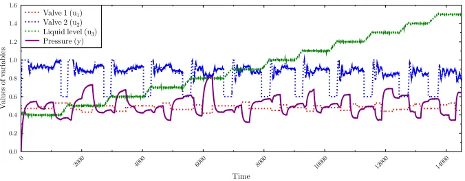
Fig. 1.Recorded values of the input variables (valves 1 and 2, Liquid level) and system
variable (pressure) of the gas-liquid separator system. Input variables are plotted with dotted lines, the system variable is plotted with a continuous line.
observations into a table of lagged input and output vector pairs. The columns of the table are as described by the vectorx(k)from Eq. 1. Each row of the table corresponds to a
point in time where an observation has been made (see Tab. 1).
The external dynamics approach allows us to formulate the task of system identifica-tion as a regression task, where we want to predict the values of the system variables from the lagged values of the system and input variables. The dependent (response) variable isy(k), while the independent variables are gathered in the vectorx(k). The data used
to learn the regression functiony(k) =f(x(k))are taken from the recorded behavior as
described above.
2.3. Data Stream Mining
Data stream mining is a sub-field of data mining, which is concerned with the develop-ment of methods for modeling of data arriving in the form of a stream [3]. Mining a data stream is substantially different from classical data mining, mainly in the way data is
Table 1.An excerpt from the recorded behavior of the GLS system depicted in Fig. 1,
reformulated according to the external dynamics approach. k
. . .
506 507 508 509 510 511 512 513 514
. . . u1 (k−3) 0.47 0.47 0.47 0.47 0.47 0.49 0.49 0.49 0.49
u1 (k−2) 0.47 0.47 0.47 0.47 0.49 0.49 0.49 0.49 0.49
u1 (k−1) 0.47 0.47 0.47 0.49 0.49 0.49 0.49 0.49 0.49
u2 (k−3) 0.8985 0.9025 0.9070 0.9070 0.9070 0.9070 0.9070 0.9120 0.9125
u2 (k−2) 0.9025 0.9070 0.9070 0.9070 0.9070 0.9070 0.9120 0.9125 0.9130
u2 (k−1) 0.9070 0.9070 0.9070 0.9070 0.9070 0.9120 0.9125 0.9130 0.9135
u3 (k−3) 0.399 0.3995 0.4 0.4 0.4 0.4 0.4 0.4005 0.4005
u3 (k−2) 0.3995 0.4 0.4 0.4 0.4 0.4 0.4005 0.4005 0.4005
u3 (k−1) 0.4 0.4 0.4 0.4 0.4 0.4005 0.4005 0.4005 0.4005
y(k−3) 0.5463 0.5463 0.5463 0.5465 0.5465 0.5463 0.5463 0.5468 0.546
y(k−2) 0.5463 0.5463 0.5465 0.5465 0.5463 0.5463 0.5468 0.546 0.5445
y(k−1) 0.5463 0.5465 0.5465 0.5463 0.5463 0.5468 0.546 0.5445 0.543
available. In the classical batch-learning data mining setting, a fixed and complete dataset is given as input to a learning algorithm, which can then use the data in an unrestricted fashion. The examples or data points are assumed to all come from the same probability distribution. In contrast to classical data mining, where all the data is available from the beginning of the process, in the on-line approach data stream mining the data instances arrive sequentially in time.
The key properties of data streams and on-line learning are:
1. the examples (data points) arrive sequentially,
2. the (data mining) algorithm has no control over the order of arrival of the examples, 3. there can potentially be arbitrarily many examples,
4. the distribution of examples need not be stationary, 5. there is a need for a response in real-time, and
6. after an example is processed it is discarded or archived – we can not access it directly, unless we explicitly store it into memory (which is comparatively small comparing to the number of examples).
3.
Modeling Dynamical Systems in Discrete Time Using Data
Stream Mining
The task of discrete-time modeling of nonlinear dynamical systems from measured data has been approached using different regression techniques. Approaches used for this pur-pose include the basis-function approaches of Artificial Neural Networks [14] and fuzzy modeling, as well as the nonparametric approaches of kernel methods [2] and Gaussian Process models [16].
The task of system identification, as defined in the previous subsection, matches the properties of learning models on data streams almost to the letter (see Sec. 2.3). This al-lows us to formulate the task of modeling dynamical systems in discrete time using data stream mining algorithms. If we observe a dynamical system, the individual data points arrive sequentially along the time dimension: The system identification (learning) algo-rithm has no control over the order of arrival of the examples/observations. Depending on whether we continue to observe the system as time goes by, there can potentially be in-finitely many examples. Depending on how frequently we make observations, the amount of data collected can easily grow over the available storage capacity. Finally, the laws underlying the behavior of a given system can change over time, especially if external disturbances appear in its environment (e.g., a pollution introduced into an ecosystem). Such dynamical systems are called time-varying dynamical systems.
To address the task of system identification using data stream mining, we use algo-rithms for learning tree-like models for regression [9,10]. They can learn model trees, as well as option trees for regression, and can also detect changes in the streaming data. Here, we briefly describe the algorithms that we use for modeling of dynamical systems.
3.1. FIMT-DD: Learning Model Trees with Change Detection
y(k−1)
u3(k−1) y(k−3)
y(k) = 0.27
y(k) = 0.29 y(k) = 0.44 y(k) = 0.61 <0.30 ≥0.30
<1.51 ≥1.51 <0.54 ≥0.54
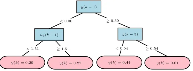
Fig. 2.An example regression tree learned on data from the gas-liquid separator domain.
splits), and leaves, which contain predictive models (constant for regression or linear for model trees) for the value of the dependent variable. An example regression tree, learned on the gas-liquid separator dataset is shown in Fig. 2.
The pseudo code of the FIMT-DD algorithm can be found in Alg. 1. The key points of the algorithm are the selection of splits for the internal nodes, the learning of linear models in the leaf nodes and the detection of changes. Algorithms for learning trees on data streams use statistical tests to determine when enough examples have been accumulated to make a split decision.
Algorithm 1The FIMT-DD algorithm. pseudocode.
Input: δ– confidence level,Nattr– number of attributes,nmin– chunk size. Output: T – root node of the current model/regression tree
for∞do
e←ReadN extExample()
Leaf←T raverse(T, e)
Seen←SeenAtLeaf(Leaf) + 1
U pdateStatistics(Leaf, e)
U pdateLeaf(Leaf, e)
ifSeen modnmin= 0then fori= 1→Nattrdo
hi←F indBestSplitF orAttribute(i)
end for
hA←BestSplit(h1, . . . , hNattr) hB ←SecondBestSplit(h1, . . . , hNattr) if VR(hA)
VR(hB) <1−
q
ln(1/δ) 2·Seenthen M akeSplit(hA, T)
Algorithms for learning decision trees on data streams start with a single leaf node. Leaves are then split when enough evidence has accumulated that the more complex tree resulting from the split will perform better than the leaf node. Deciding when to split a leaf is a critical step in tree construction. For this purpose, FIMT-DD utilizes the variance reduction heuristic along with the Hoeffding bound [6].
The basic version of FIMT-DD learns regression trees, where the predictions in the leaves are constant. An extension of the FIMT-DD algorithm learns model trees instead of regression trees. In model trees, at a given leaf, instead of returning the average of target variable values for the accumulated examples, we use linear regression to predict the target value of incoming examples.
To this end, we place a single layer perceptron into each leaf. Given inputsx1, . . . , xn
(attribute values), the output is computed as o = Pn
i=1xiwi +b, where wi are the
weights andbis the threshold. Using the squared error function for an examplee,E(x) =
1 2(y−o)
2, whereyis the actual target value andois the predicted target value, we can con-tinuously update the perceptron according to thedeltaorWidrow-Hoff additive rule. The
complete perceptron learning scheme (procedureU pdateLeafin Alg. 1) is as follows
1. The weightsw1, . . . , wnand the thresholdbare initialized to random values.
2. Consider a vectorx= (x1, . . . , xn)and calculateo.
3. Update the weights using the delta rulew←w+η(y−o)x,(ηis thelearning rate).
4. Return to step 2.
In our case, the learning rate is not kept constant but is decreased inversely propor-tional to the number of instancesη = η0
1+N ηd, whereη0is the initial learning rate,N is the number of examples processed andηdis the learning rate decay parameter.
To detect changes, FIMT-DD makes use of the Page-Hinckley test (see Alg. 2). The test is a mechanism for detecting changes in a signalx(k). At any time pointk, the test
considers the following two variables: a cumulative sum m(k)and its minimal value
M(k) = mini=1,...,km(i). The summ(k)is defined as the cumulative difference between
the signalx(k)and its averagex(k)corrected with an additional parameterα(minimal
absolute amplitude of change that we wish to detect),m(k) =Pk
i=1(x(k)−x(k)−α). The Page-Hinckley test monitors the difference betweenm(k)andM(k),P H(k) =
m(k)−M(k).When this difference passes a thresholdλ, an alarm is triggered which
informs the algorithm of a possible change. To detect possible change in the data, we use the Page-Hinckley test on the absolute error signal|y−yˆ|, whereyis the true value of
an example andyˆis the predicted value. The error is back-propagated towards the root of
the tree, as the Page-Hinckley test is monitored at each node in the tree.
When an alarm is triggered, the FIMT-DD algorithm responds by starting to grow an alternate subtree. The tree is grown at the node at the lowest level which has triggered the alarm. The alternate tree is grown in parallel with the original subtree, while the growth of the original subtree is stopped. At a time interval ofTmin, the viability of both the original Oand the alternate treeAis compared using the fadedQistatistic. IfQi(O, A)is greater
than0, that means that the alternate subtree is better in terms of the predictive performance
and the original subtree is replaced with the alternate. However, if after10·Tminexamples,
Algorithm 2Traverse procedure of the FIMT-DD algorithm. pseudocode.
Input: T – node (root, internal or leaf),e– training example Output: Leaf– leaf node where the exampleewill be traversed
ifIsLeaf(T)6=T ruethen
Change←U pdateP HT est(T, e)
ifChange=T ruethen InitiateAlternateT ree(T, e)
end if
Child←ApplyN odeT estT oExample(T, e)
Leaf←T raverse(Child, e)
else
Leaf←T end if return Leaf
3.2. ORTO: Learning Option Trees for Regression on Data Streams
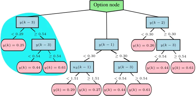
The ORTO algorithm is an extension of the FIMT-DD algorithm which introduces option nodes into the learned regression (or model) trees [10]. When making a prediction for a new example with a regular regression (or model) tree, the example is sorted down exactly one branch of the tree, i.e., sorted to exactly one branch of each internal node it encounters. In contrast, when sorting an example through an option node, the example is multiplied and sorted to each of the children of an option node. This means that in each option node multiple predictions are produced, corresponding to the multiple branches out of the node followed by the example. These predictions are then aggregated to form a single prediction, e.g., by averaging. An example option tree for regression is presented in Fig. 3.
Option node
y(k−1)
≥0.30 <0.30
u3(k−1)
≥1.51
y(k) = 0.29 y(k) = 0.27 <1.51
y(k−3)
≥0.54
y(k) = 0.44 y(k) = 0.61 <0.54
y(k−3)
y(k−3) y(k) = 0.25
<0.29
≥0.54
y(k) = 0.44 y(k) = 0.61 <0.54
≥0.54
y(k−2)
y(k−3) y(k) = 0.26
<0.30
≥0.54
y(k) = 0.44 y(k) = 0.61 <0.54
≥0.30
Fig. 3.An example option tree learned on data from the gas-liquid separator domain.
The pseudocode of ORTO is presented in Alg. 3. The split decision process of ORTO is almost identical to that of FIMT-DD, but it includes an important alteration, which allows the introduction of option nodes. We use two aggregation approaches, averaging and choosing the best path.Averagingis the more straightforward of the two approaches.
The final prediction of the option node is obtained by averaging the predictions obtained from the children of the option node. We refer to this variant of the ORTO algorithm as
ORTO-A. The other aggregation approach used is tochoose the (currently) best path. The
cumulative errors for each example processed are kept for each of the children of an option node, and when combining the predictions, the prediction of the child with currently the
Algorithm 3The ORTO algorithm. pseudocode.
Input: δ – confidence level,Nattr– num. of attributes,nmin– chunk size,Agg– aggregation method,β– option decay factor,Tmax– max. number of options.
Output: T – current option tree. T←InitiateOptionT ree()
for∞do
e←ReadN extExample()
Leaf←T raverse(T, e)
Seen←SeenAtLeaf(Leaf) + 1
U pdateStatistics(Leaf, e)
U pdateLeaf(Leaf, e)
ifSeen modnmin= 0then fori= 1→Nattrdo
hi←F indBestSplitF orAttribute(i)
end for
hA←BestSplit(h1, . . . , hNattr) hB ←SecondBestSplit(h1, . . . , hNattr) if VR(hA)
VR(hB) <1−
q
ln(1/δ) 2·Seenthen M akeSplit(hA, T)
else
O←CreateOptionN ode(T, Leaf)
AddSplit(hA, O)
Count←0
k←CountSplitCandidates(h1, . . . , hNatr) l←Level(T, Leaf)
fori= 1→Nattrdo
if i 6= 1 and Count < k · βl and VR(hi)
VR(hA) > 1 −
q
ln(1/δ) 2·Seen and N umberOf Options(T)< Tmaxthen
AddSplit(hi, O)
Count←Count+ 1
end if end for end if end if
return P redict(T, Agg, e)
lowest error is returned as the option node’s prediction. For example, the leftmost child of the option node of the tree in Fig. 3 has the lowest error and would be used when making predictions. This variant of ORTO is referred to asORTO-BT.
4.
Case Studies
In this paper, we demonstrate the applicability of tree-based approaches to on-line regres-sion to the task of system identification in discrete-time, on three use cases coming from the area of control engineering. These include the following case studies: modeling the gas-liquid separator [11], modeling the process of pH neutralization [5], and modeling a synthetic dynamical system [13]. Below we present briefly each of the case studies.
4.1. Case Study: Gas-Liquid Separator
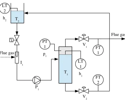
The gas-liquid separator is a unit in a semi-industrial process plant which is part of a larger pilot plant. The unit’s purpose is to capture flue gases under low-pressure from the effluent channels using a water flow, cool the gases down, and supply them with higher pressure to other parts of the plant. A schematic representation of the unit is given in Fig. 4.
The flue gases coming from the effluent channels are absorbed by the water into the water circulation pipe through the injectorI1. The water flow is produced by the water ring pumpP1, which operates at constant speed. The gas-water mixture is fed by the pump into the tankT1, where the gas-liquid separation occurs. The accumulated gases form a pressurized gas ‘cushion’. This pressure forces the flue gases to be blown out from the tank into a neutralization unit. Similarly, the cushion pushes the water to circulate back into the reservoir. The amount of water in this circuit is kept constant. The entire process is controlled through a manipulation of theV1andV2valves.
This process is modeled with a set of differential equations [11], one of which is presented below: The equation describes the rate of change of the p1 variable, which
T2
T1 Flue gas
P1
V2 V1
Flue gas
I1
PT 1 p1
LT 1 h1
FT 1
FT 2 LT
2 h2
corresponds to the relative air pressure in the tankT1
dp1
dt =fa(h1)· h
α1+α2p1+α3p21+fb(u1)
√
p1+fc(u2)
p
p1+α4+α5h1
i
, (2)
whereh1is the liquid level inT1,u1andu2are the command signals for theV1andV2 valves, respectively,α1, . . . , α5 are constants, while fa,fb andfc are functions of the
appropriate variables. In more detail,fa is a rational function ofh1, whilefbandfcare
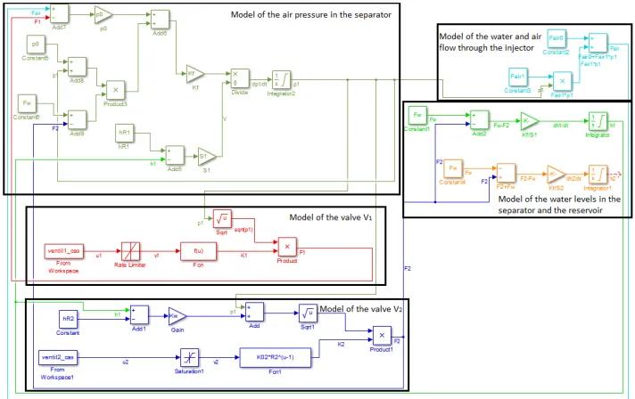
valve characteristics, i.e., exponential functions of input signalsu1andu2, respectively. In previous work, a complete non-linear dynamic model was derived and modeled in MATLAB by using Simulink [17]. The model consists of several parts: models of the valvesV1andV2, a model of the air pressure in the separator, a model of the water and air flow through the injector, and a model of the water levels in the separator and the reservoir (see Fig. 5). For the purpose of comparison, we replicated the simulation model using the same parameters (see Sec. 5).
The modeling task in this case study is to build a predictive model that can predict the valuep1from its previous (lagged) values, as well as the current and previous values of the input variables. For the purpose of modeling,h1was also taken as an input variable, in addition to the control signalsu1andu2for the valvesV1 andV2. For this dataset a system lag of3was selected.
The dataset is composed of two runs of the gas-liquid separator, each sampled twice per second for about two hours, netting around14500examples each. For the purposes
of learning a predictive model, we have concatenated these two runs into a single dataset, producing29036total examples.
4.2. Case Study: pH Neutralization
This case study [5] is concerned with the problem of controlling alkalinity, a common problem in biotechnological and chemical processes. In particular, it seeks to identify the pH neutralization process, which exhibits severe nonlinear behavior.
The system is composed of several fluid streams: an acid streamQ1, a buffer stream
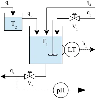
Q2and a base streamQ3. The streams are mixed in a tankT1. Prior to the mixing, the acid stream passes through another tankT2. The observed variable is the effluent pH, which is controlled by manipulating the flow rate of the base streamQ3, while both the acid and the buffer flows are kept constant. This process is schematically presented in Fig. 6.
The model of this dynamical system [5] contains the following state, input (control) and output variables:x= [Wa4, Wb4, h1], u=Q3, y=pH , whereWa4andWb4are the effluent reaction invariants andh1is the liquid level in the tankT1. Following from here, it is assumed that a (previously designed) controller is being used to keep the fluid level in the tankT1constant ath1= 14cm. This is achieved through the manipulation of the flow rate of the effluent streamQ4.
The mathematical model obtained has the following form:
x=f(x) +g(x)u
c(x, y) = 0, (3)
wheref(x) andg(x)are non-linear functions of the state vectorx, while c(x, y) is a
non-linear function that implicitly defines the value of the output variabley.
In total, a set of31998data instances was produced by simulating the above model.
We apply the lagging procedure with a system lag of2. This provides4features to be used
in the modeling of the system behavior, i.e.,y(k−1),y(k−2),u(k−1)andu(k−2).
q1 q2
q3
q4 q1'
h1
T
2T
1LT
pH
V1V2
4.3. Case Study: Narendra
To evaluate how the FIMT-DD algorithm adapts to change, we consider the synthetic Narendra dataset [13]. This dynamical system is composed of an input variableuand a
system variabley, connected as follows
y(k) = 1
1 +y(k−1)2 +u(k−1)
3. (4)
The value of the input variableuis selected uniformly at random from the interval[−1,1]
after every20examples (time points) and kept constant for the next 20 examples. The
initial system state is set asy(0) = 0. This system is modeled with a system lag of1,
which gives us two featuresy(k−1)andu(k−1)to model the system behavior.
Specifically to test the change detection and adaptation of FIMT-DD, we change the dynamics of the system. There are two types of changes that we introduce: change of the function and change of a parameter. In the former, the recurrence relation is replaced by
ˆ
y(k) = 1
1 + ˆy(k−1)2+u(k−1), (5)
replacing the exponent 3 in the second term with a value of1, while in the latter, the
relation changes into
ˆ
y(k) = 1
1 + ˆy(k−1)2 +2u(k−1)
3, (6)
replacing the constant1in front of the second term with the constant2.
For this case study we generated datasets Narendra-F and Narendra-P, where the change is introduced in the function and in the parameter, respectively. Both types of changes are introduced half-way through the dataset. In total,900000instances were
gen-erated and in both cases the change was introduced at the450000th time point.
When considering these two datasets, we compare two variants of the FIMT-DD algo-rithm, with an enabled and disabled change adaptation mechanism, respectively. In both cases, we use FIMT-DD to learn model trees.
5.
Experimental Design
In this section, we first explicitly state the experimental questions that we set out to an-swer. We then list the on-line regression algorithms that we evaluate and compare, along with their parameter settings. The section concludes with the evaluation methodology.
5.1. Experimental Questions
we wish to evaluate the effectiveness of the change detection mechanism of the on-line tree learning approach, which would be necessary for the identification of time-varying dynamical systems.
To answer the question of whether the considered approaches perform satisfactorily on the task of identification of dynamical systems, we need to verify that they make small, preferably ever-decreasing, errors. Low values of the error are desired that should be lower than those of a pre-selected baseline method. This means accurate predictions of the evolution of the state of the system, i.e., its state at the next point in time.
To evaluate which of the algorithms performs best, we compare them on two bench-mark control engineering problems. The first one consists of measured data (gas-liquid separator case study in Sec. 4.1), while the second is synthetic (pH neutralization case study in Sec. 4.2). Our task is primarily to examine the predictive performance of the algorithms. In addition, we also inspect their time and memory consumption.
For the gas-liquid separator case study, we compare the simulation of the system dy-namics obtained by using the models learned by data stream mining with the simulation produced by the expert model described in Sec. 4.1. This allows us to determine whether the learned model, which required almost zero effort to create, captures the dynamics of the system and how it compares to the expert model, which required a lot of effort to produce.
Specifically, we use the best performing algorithm identified above (ORTO-A), which learns on only the first run of the gas-liquid separator. Similarly, the parameter tuning of the expert model is performed on the first run. The second run of the gas-liquid separator is used for the simulation. For the learned model, the lagged output values are replaced by its earlier predictions, i.e., aside from the initial system state, the learner is agnostic of the recorded state of the system during the second run.
Finally, an important aspect of learning from data streams is the ability to detect changes in the data. In the context of system identification, this corresponds to the suc-cessful identification of time-varying dynamical systems. We investigate the performance of on-line learning of model trees with and without change detection on an artificial task where two types of changes are introduced to a known dynamical system (see Sec. 4.3).
5.2. Evaluated Algorithms
We compare and evaluate the on-line regression algorithms described in Sec. 3. In partic-ular, we compare FIMT-DD using regression and model trees as well as the ORTO-A and ORTO-BT algorithms for learning option trees, without change detection, on the pH neu-tralization and gas-liquid separator case studies. For the Narendra case study, we consider only FIMT-DD with and without change detection.
We use a single linear regression model learned on-line as a baseline, i.e., a single perceptron (see Sec. 3.1). It can also be interpreted as a model tree with only leaf at the root, which is never allowed to grow. The parameter settings chosen for the evaluated algorithms are listed in Tab. 2.
5.3. Evaluation on Data Streams
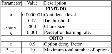
Table 2.Parameter settings used for the compared algorithms.
Parameter Value Description
FIMT-DD δ 0.0000001Confidence level.
τ 0.05 Tie threshold.
nmin 300 Chunk size.
η 0.001 Perceptron learning rate.
ORTO
β 0.9 Option decay factor.
Tmax 10 Maximum total number of options.
fading factor into the calculation of error metrics [3]. Instead of reporting the average errorEN = N1 P
N
i=1L(yi,yˆi), whereL is some loss function,yi is the real value of
thei-th example andyˆiis the algorithm’s prediction on thei-th example, we introduce
the faded sum of errorsSN and the faded number of examplesBN defined as follows: SN =L(yN,yˆN)+αSN−1=P
N i=1α
N−iL(y
i,yˆi),BN = 1+αBN−1=P
N i=1α
N−i,
to compute the faded errorEN =BSNN. We use the parameter valueα= 0.975[3].
If we use the square loss functionL(y,yˆ) = (y −yˆ)2, this allows us to compute the faded mean squared error. Additionally, we use the relative root mean squared error (RRMSE), where we take the square root of the ratio of the mean squared error of the algorithm with the mean squared error of the linear regression model, which is used as a baseline:RRM SE=qM SEalg
M SElr .
6.
Results and Discussion
In this section, we present the experimental results organized according to the experimen-tal questions, posed in the previous section. We first discuss the question of the satisfactory performance of data stream mining approaches for modeling dynamical systems. Next, we discuss the relative performance of the different approaches to on-line regression. After-wards, we focus on the comparison of two simulations obtained by a learned and a human constructed model. Finally, we discuss how the on-line learning of regression trees (with and without change detection) deals with time varying dynamical systems.
6.1. Comparison to the Baseline
In Tab. 3, we present the faded mean squared errors for the baseline method of linear regression and each of the four tree-based approaches for the gas-liquid separator do-main. The error is recorded after each5000examples. The performance figures for the
pH domain are given in Tab. 4.
Table 3.The faded mean squared errors of the different modeling approaches on the
gas-liquid separator dataset, recorded at intervals of5000examples.
# of examples 5000 10000 15000 20000 25000
Baseline 0.0084 0.0051 0.0253 0.0117 0.0136
FIMT-DD Reg. trees 0.0064 0.0018 0.0050 0.0030 0.0011
FIMT-DD Model trees0.0040 0.0007 0.0006 0.0016 0.0003
ORTO-A 0.0008 0.0002 0.0021 0.0002 0.0005
ORTO-BT 0.0022 0.0002 0.0018 0.0011 0.0018
neutralization case, the error is getting close to zero for the tree-based approaches, but stays very high for the linear regression baseline approach.
The relative root mean square error essentially compares the error of the tree-based approaches to the error the baseline, the latter having the root relative root mean square error of1. For the gas-liquid separator domain, the relative root mean squared error is
clearly lower than 1for all tree-based approaches (see Fig. 7a). For the pH
neutraliza-tion case it is even lower (see Fig. 7b). To sum up, we can conclude that all tree-based approaches perform successfully at the task of system identification in discrete-time.
6.2. Relative Performance of the Tree-Based Approaches
In this section, we present the performance of the tree-based methods in terms of the (faded) root relative mean squared error with respect to the baseline (see Fig. 7), memory and time consumption (see Fig. 8 and 9), both for the gas-liquid separator case (marked with (a) in the figures) and the pH neutralization case (marked with (b) in the figures).
For the case of the FIMT-DD algorithm, we can see that FIMT-DD clearly performs better when learning model trees than when learning regression trees (see Fig. 7). Further-more, the usage of model trees makes learning faster (in terms of achieving lower error with the same number of examples). In addition, model trees also achieve lower error overall than regression trees (for any given number of examples).
Regarding the option trees, the ORTO-A algorithm clearly outperforms the ORTO-BT algorithm. While the option trees learned for both ORTO-A and ORTO-BT are the same, the aggregation by averaging yields more accurate predictions. In addition, ORTO-A is also less prone to fluctuations in the error.
Table 4.The faded mean squared errors of the different modeling approaches on the pH
dataset, recorded at intervals of5000examples.
# of examples 5000 10000 15000 20000 25000 30000
(a)gas-liquid separator dataset (b)pH dataset
Fig. 7.The relative performance (in terms of RRMSE) of the different approaches.
If we analyze the overall performance, the ORTO-A algorithm is the best performing algorithm. It consistently outperforms all of the other algorithms in terms of the error. In addition, is the fastest among the algorithms to achieve low errors. These results hold both for the gas-liquid separator case, as well as the pH neutralization case. This is to be expected, as the ORTO algorithm was designed to overcome the problem of initial delay in learning in a streaming setting and to increase the predictive accuracy faster [10].
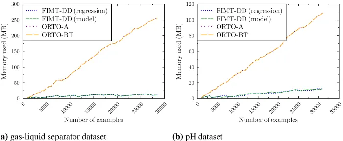
If we analyze the performance in terms of time and memory used, we can observe that the ORTO-A and the ORTO-BT algorithms are the most resource intensive (see Fig. 8 and 9). However, the ORTO-BT algorithm uses a fractionally smaller part of the tree for prediction than the ORTO-A algorithm. Using model trees rather than regression trees, for the FIMT-DD algorithm, increases the time consumption slightly, while the memory consumption barely changes.
(a)gas-liquid separator dataset (b)pH dataset
(a)gas-liquid separator dataset (b)pH dataset
Fig. 9.The time consumption (in seconds) of the different tree-based approaches.
6.3. Comparison to the Simulated Model
Here we use ORTO-A, which we identified as the best performing method. Here, we com-pare its predictions to the recorded values, as well as the values obtained by simulating the expert-derived non-linear dynamic model (see Sec. 4.1). The simulation was performed in Simulink using the ODE3 (Bogacki-Shampine) fixed step solver.
The results of the comparison are presented in Fig. 10. It is clear that the model learned by ORTO-A captures the dynamics of the system. In the first half of the simulation, the pressure simulated by the learned model is often off of the real pressure. This may be due to the differences between the two runs of the gas-liquid separator.
While the simulation of the expert-derived model better captures the dynamics of the system, it should be noted that the construction of this model required a lot of human resources. Our method, on the other hand, was used out of the box, without any param-eter tuning, requiring minimal additional resources, both in terms of human effort and computation time.
6.4. Change Detection
In Fig. 11, we show the performance of the FIMT-DD algorithm in terms of the faded mean squared error on the Narendra-F and Narendra-P datasets, from the Narendra case. In the former, a functional form of the dynamics is changed, while in the latter a parameter of the dynamics changes, to simulate a time-varying dynamical system (see Sec. 4.3)
Analyzing the performance of the Narendra-F dataset, we notice that the FIMT-DD algorithm with change detection does detect the change, builds an alternate subtree and replaces the original in about25000examples, as the change is introduced at the450000
-th example and -the predictive accuracy increases at about -the 475000th example (see
Fig. 11a). However, the difference in the error between the FIMT-DD with and without detection and the adaptation to change is small. The increase in error due to the abrupt change in the dynamics, which is in this case also relatively small, peaks at about0.08.
Fig. 10.The recorded values of the system variable (pressure) and its values simulated
by the model learned by ORTO-A and the constructed expert model of the pressure in the gas-liquid separator case study.
the range of the second term to [−2,2], while the change introduced in the
Narendra-F dataset only changed its distribution on the[−1,1]interval. As before, the change is
detected and the tree is adapted in about25000examples. Because the introduced change
is more radical than before, regrowing of the affected subtree(s) produces better results.
7.
Conclusions and Further Work
The central question addressed by this paper concerns the applicability of the paradigm of mining data streams, and in particular the tree-based approaches to on-line regression, to the task of system identification in discrete-time. To address this question, we perform a thorough experimental evaluation, where we applied several tree-based approaches for on-line regression to several benchmark problems in discrete-time modeling of dynamical
(a)Narendra-F dataset (b)Narendra-P dataset
systems. Using an evaluation methodology and performance measures appropriate for the task at hand, we answer several experimental questions, as summarized below.
Our conclusions are as follows. Overall, tree-based approaches to on-line regression are appropriate for solving the task of identification of dynamical systems in discrete-time. Among the considered approaches, the ORTO-A algorithm clearly stands out as the best-performing one. ORTO-A learns option trees for regression, where an example may be sorted down multiple branches of the tree in option nodes, and averages the predictions obtained from each of the branches in the option tree that an example follows.
When comparing the learned model to an expert constructed model, we noted that the expert model produces a simulation closer to the recorded data. However, the learned model still captures the dynamics of the system quite well. Furthermore, the learned model required minimal additional use of resources, human and machine, while the con-struction of the expert model and its parameter tuning is a labor intensive and error-prone process.
We also investigate the use of tree-based regression algorithms on data streams for the identification of time-varying systems. The FIMT-DD algorithm for learning model trees is applied to synthetic data, which include a change of system dynamics at a given point in time. The change detection mechanism and the adaptation method in the FIMT-DD algorithm successfully detect the introduced change and adapt the tree to achieve better performance (as compared to the FIMT-DD algorithm without change detection).
Many avenues remain for further work. Specifically, the change detection and adap-tation mechanisms of tree-based on-line learning approaches should be tested on other real-world datasets, where change is either known or suspected to appear. Furthermore, the mechanism for detecting change, i.e., the Page-Hinckley test, should be automatically parameterized with regard to the relative error instead of the absolute error, as this would allow to detect changes of any size without the need to select the parameters manually.
More generally, the experimental questions posed in this paper should be answered for a larger set of real-world problem domains and corresponding datasets. Of particular interest is the identification of dynamical systems which have more than one system vari-able: These are called MIMO (multiple input multiple output systems). Additional on-line learning methods should also be considered for the task at hand, such as tree-based on-line ensemble approaches, including on-on-line methods for learning multi-target regression and model trees on data streams [8].
Acknowledgments.Aljaˇz Osojnik is supported by the Slovenian Research Agency (ARRS) through a young researcher grant. Saˇso Dˇzeroski would like to acknowledge the financial support of the following institutions: The Slovenian Research Agency (Grant P2-0103), the European Commission (Grants ICT-2013-612944 MAESTRA and KT-2013-604102 HBP). The authors would also like to thank Juˇs Kocijan for providing the expert simulation model for the gas-liquid separator use case and the provided feedback.
References
1. Breiman, L., Friedman, J.H., Olshen, R.A., Stone, C.J.: Classification and Regression Trees. Wadsworth, Belmont, CA (1984)
3. Gama, J.: Knowledge Discovery from Data Streams. Chapman & Hall/CRC, London (2010) 4. Gama, J., Sebasti˜ao, R., Rodrigues, P.P.: Issues in evaluation of stream learning algorithms.
In: Proceedings of the 15th ACM SIGKDD International Conference on Knowledge Discovery and Data Mining. pp. 329–338. ACM Press, New York (2009)
5. Henson, M.A., Seborg, D.E.: Adaptive nonlinear control of a pH neutralization process. IEEE Transactions on Control Systems Technology 2, 169–182 (1994)
6. Hoeffding, W.: Probability inequalities for sums of bounded random variables. Journal of the American Statistical Association 58, 13–30 (1963)
7. Ikonomovska, E.: Algorithms for Learning Regression Trees and Ensembles on Evolving Data Streams. Ph.D. thesis, Joˇzef Stefan International Postgraduate School, Ljubljana (2012) 8. Ikonomovska, E., Gama, J., Dˇzeroski, S.: Incremental multi-target model trees for data streams.
In: Proceedings of the 2011 ACM Symposium on Applied Computing. pp. 988–993. ACM Press, New York (2011)
9. Ikonomovska, E., Gama, J., Dˇzeroski, S.: Learning model trees from evolving data streams. Data Mining and Knowledge Discovery 23, 128–168 (2011)
10. Ikonomovska, E., Gama, J., ˇZenko, B., Dˇzeroski, S.: Speeding-up Hoeffding-based regression trees with options. In: Proceedings of the 28th International Conference on Machine Learning. pp. 537–544. ACM Press, New York (2011)
11. Kocijan, J., Likar, B.: Gas-liquid separator modelling and simulation with Gaussian-process models. Simulation Modelling Practice and Theory 16, 910–922 (2008)
12. Kohavi, R., Kunz, C.: Option decision trees with majority votes. In: Proceedings of the 14th In-ternational Conference on Machine Learning. pp. 161–169. Morgan Kaufmann, San Francisco, CA (1997)
13. Narendra, K., Parthasarathy, K.: Identification and control of dynamical systems using neural networks. IEEE Transactions on Neural Networks 1, 4–27 (1990)
14. Nelles, O.: Nonlinear System Identification: From Classical Approaches to Neural Networks and Fuzzy Models. Springer, Berlin (2001)
15. Quinlan, J.R.: Learning with continuous classes. In: Proceedings of the 5th Australian Joint Conference On Articial Intelligence. pp. 343–348. World Scientific, Singapore (1992) 16. Rasmussen, C., Williams, C.: Gaussian Processes for Machine Learning. MIT Press,
Cam-bridge, MA (2006)
17. Vranˇci´c, D., Juriˇci´c, D., Petrovˇciˇc, J.: Measurements and mathematical modelling of a semi-industrial liquid-gas separator for the purpose of fault diagnosis. Tech. rep., Joˇzef Stefan Insti-tute, Ljubljana, Slovenia (1996), dP-7260
Aljaˇz Osojnikis a young researcher at the Department of Knowledge Technologies, Joˇzef
Stefan Institute, Ljubljana, Slovenia and a PhD student at the Joˇzef Stefan Postgraduate School. He completed his MSc and BSc in mathematics at the Faculty of Mathematics and Physics, University of Ljubljana, Slovenia. His research interests are related to machine learning, data mining, and more specifically development of methods for data stream mining.
Panˇce Panovis a postdoctoral researcher at the Department of Knowledge Technologies,
the process of knowledge discovery, which can be employed in various applications. He was actively involved in several EU-funded projects in the past (IQ, SUMO) and is cur-rently involved in the MAESTRA project. In addition, he participated in several projects financed by the Slovenian research agency and one bilateral project between Slovenia and Croatia. He is a co-editor of the book entitled “Inductive databases and constraint-based data mining” published in 2010 by Springer. In 2014, he was program co-chair of the International Conference on Discovery Science (2014) and co-editor of the proceedings of the conference published by Springer. Finally, in 2016 he a co-editor of a special issue of the Journal Machine Learning on Discovery Science.
Saˇso Dˇzeroskiis a scientific councillor at the Joˇzef Stefan Institute and the Centre of
Ex-cellence for Integrated Approaches in Chemistry and Biology of Proteins, both in Ljubl-jana, Slovenia. He is also a full professor at the Joˇzef Stefan International Postgraduate School. His research is mainly in the area of machine learning and data mining (including structured output prediction and automated modeling of dynamic systems) and their appli-cations (mainly in environmental sciences, incl. ecology, and life sciences, incl. systems biology). He is co-author/co-editor of more than ten books/volumes, including “Inductive Logic Programming”, “Relational Data Mining”, “Learning Language in Logic”, “Com-putational Discovery of Scientific Knowledge” and “Inductive Databases and Constraint-Based Data Mining”. He has participated in many international research projects (mostly EU-funded) and coordinated two of them in the past: He is currently the coordinator of the FET XTrack project MAESTRA (Learning from Massive, Incompletely annotated, and Structured Data) and one of the principal investigators in the FET Flagship Human Brain Project.