CSUSB ScholarWorks
CSUSB ScholarWorks
Electronic Theses, Projects, and Dissertations Office of Graduate Studies
12-2017
Making Models with Bayes
Making Models with Bayes
Pilar Olid
Follow this and additional works at: https://scholarworks.lib.csusb.edu/etd
Part of the Applied Statistics Commons, Multivariate Analysis Commons, Other Applied Mathematics Commons, Other Mathematics Commons, Other Statistics and Probability Commons, Probability
Commons, and the Statistical Models Commons
Recommended Citation Recommended Citation
Olid, Pilar, "Making Models with Bayes" (2017). Electronic Theses, Projects, and Dissertations. 593.
https://scholarworks.lib.csusb.edu/etd/593
A Thesis
Presented to the
Faculty of
California State University,
San Bernardino
In Partial Fulfillment
of the Requirements for the Degree
Master of Arts
in
Mathematics
by
Pilar Olid
A Thesis
Presented to the
Faculty of
California State University,
San Bernardino
by
Pilar Olid
December 2017
Approved by:
Dr. Charles Stanton, Committee Chair
Dr. Jeremy Aikin, Committee Member
Dr. Yuichiro Kakihara, Committee Member
Dr. Charles Stanton, Chair, Department of Mathematics
Abstract
Bayesian statistics is an important approach to modern statistical analyses. It
allows us to use our prior knowledge of the unknown parameters to construct a model for
our data set. The foundation of Bayesian analysis is Bayes’ Rule, which in its proportional
form indicates that the posterior is proportional to the prior times the likelihood. We will
demonstrate how we can apply Bayesian statistical techniques to fit a linear regression
model and a hierarchical linear regression model to a data set. We will show how to apply
different distributions to Bayesian analyses and how the use of a prior affects the model.
We will also make a comparison between the Bayesian approach and the traditional
Acknowledgements
First and foremost, I would like to express my gratitude to my advisor Dr.
Charles Stanton for his guidance, encouragement, patience, and support. Without his
knowledge and help this thesis would not have been possible.
Second, I want to thank the members of my committee, Dr. Jeremy Aikin and
Dr. Yuichiro Kakihara, for reviewing this thesis. Their passion for mathematics has truly
been an inspiration.
Third, I am grateful to my friends for their continuous emotional support during
my graduate journey. Without them cheering me on I would not have made it to the end.
Finally, I would like to thank my family. Without my mother and father’s
encouragement and support for my academic endeavors none of this would have been
Table of Contents
Abstract iii
Acknowledgements iv
List of Tables vi
List of Figures vii
1 Introduction 1
2 Basics of Bayesian Statistics 2
2.1 History . . . 2
2.2 Bayes’ Rule . . . 7
2.3 Making Inferences with Bayes . . . 13
2.4 Frequentist vs. Bayesians . . . 18
3 Linear Regression 21 3.1 Frequentist Regression . . . 21
3.2 Frequentist Regression Example . . . 23
3.3 Bayesian Regression . . . 25
3.4 Bayesian Regression Examples . . . 27
4 Hierarchical Linear Regression 33 4.1 Bayesian Hierarchical Linear Regression . . . 33
4.2 Bayesian Hierarchical Linear Regression Example . . . 35
5 Conclusion 40
List of Tables
2.1 Sample space for the “pascal,”“pastel,”and “castle”dice. . . 11
2.2 Adult U.S. population with diabetes from a sample ofn= 100. . . 16
3.1 Frequentist linear regression R output. . . 24
3.2 Bayesian linear regression R output with non-informative prior. . . 28
3.3 Bayesian linear regression R output with informative prior. . . 30
4.1 Frequentist Poisson linear regression R output. . . 35
4.2 R output for basic Bayesian Poisson linear regression. . . 37
List of Figures
2.1 Plots of beta prior distributions. . . 15 2.2 Prior, likelihood, and posterior densities for U.S. adults with diabetes. . . 17
3.1 Relationship between “Poverty Level”and “Number of Home Rooms”in the
frequentist model. . . 25
3.2 Trace and density plots for Intercept and Poverty for the Bayesian model
with non-informative prior. . . 29
3.3 Relationship between “Poverty Level”and “Number of Home Rooms”in the
Bayesian model with non-informative prior. . . 30
3.4 Trace and density plots for Intercept and Poverty for the Bayesian model
with informative prior. . . 31
3.5 Relationship between “Poverty Level”and “Number of Home Rooms”in the
Bayesian model with informative prior. . . 32
4.1 Relationship between “Median Income”and “Number of Home Rooms”in
the frequentist and Bayesian Poisson models. . . 36
4.2 Diagnostics plots for Bayesian hierarchical Poisson linear regression model. 38
4.3 Relationship between “HHIncomeMid”and “HomeRooms”based on
Chapter 1
Introduction
It is only in the last 60 years or so that Bayesian statistics has become popular,
but its origins date back to more than 250 years. In statistics there are two major
approached to making inferences, the frequentist paradigm and the Bayesian paradigm.
Frequentist statistics made its debut in the 1920’s and has been the go-to methods for
inferential statistics in many disciplines. It wasn’t until the mid 1900’s that Bayesian
statistics started to emerge as a practical alternative when frequentist methods fell short.
In fact, it was thanks to Bayesian statistics that Alan Turing was able to break the
German Enigma code during World War II, and that the missing Air France Flight 447
from 2009 was recovered. Like in any paradigm, there are objections to the Bayesian
approach. It is mainly criticized because it relies on subjective priors and uses variant
parameters. However, in 1992 the International Society for Bayesian Analysis (ISBA)
was founded to promote the implementation and development of Bayesian statistics. It is
because of its increase in popularity, and because of its non-fixed parameter requirement
that we will be using Bayesian statistical techniques to construct a hierarchical linear
Chapter 2
Basics of Bayesian Statistics
2.1
History
The birth of Bayesian statistics can be attributed to Thomas Bayes (1702-1761),
a Presbyterian minister and amateur mathematician. It was not Bayes’ intention to create
a new field in mathematics, he simply wanted to know how the effect of some event can
tell him thecause of that event. Without intent, however, his work sparked a 250-year-old dispute among statisticians. There were those that helped develop the theory like Pierre
Simon Laplace and Harold Jeffreys, and those that largely opposed it like Ronald Aylmer
Fisher. In any case, Bayesian statistics has helped solve famous historical events and
continues to grow as a statistical method for applied research. To understand Bayesian
statistics, however, we need to first learn about the men that created it and about the
events that helped its development.
Bayes studied theology in Scotland, at the University of Edinburgh, and upon
completing his studies he served as an assistant minister to his father who was a clergyman
of the Presbyterian Church [McG11]. During this time, he became a member of the Royal
Society, which allowed him to read and write about theological issues [McG11]. Bayes
presumably read an essay by David Hume (1711-1776) where he stated that we cannot be
certain about a cause and effect, just like we can’t be certain that God is the creator of
the world, and that we can only speak in terms of “probable cause and probable effect”
[McG11]. Bayes also read Abraham de Moivre’s (1667-1754) book Doctrine of Chances,
Bayes thought about the inverse, looking at effect to determine the cause.
Bayes wanted to use observable information to determine the probability that
some past event had occurred. Basically, he wanted to use current information to test the
probability that a hypothesis was correct. To test his idea, Bayes developed an experiment
that would allow him to quantify “inverse probability”, that is, effect and cause. The
experiment ran as follows: Bayes sits with his back towards a billiard table and asks a
friend to throw an imaginary cue ball onto the table. He then asks his friend to make a
mental note of where the imaginary ball lands and to throw an actual ball and report if
it landed toward the right or the left of the imaginary cue ball. If his friend says that it
landed to the right, then Bayes knows that the cue ball must be to the left-hand edge of
the billiard table, and if his friend says that it landed to the left of the cue ball then it
must be on the right-hand edge of the table. He continues to ask his friend to repeat this
process. With each turn, Bayes gets a narrower idea of possible places where the cue ball
lies. In the end, he concludes that the ball landed between two bounds. He could never
know the exact location of the cue ball, but he could be fairly confident about his range
of where he thought the cue ball had landed [McG11].
Bayes’ initial belief about where the cue ball is located is his hypothesis. This
location is given as a range in the form of a probability distribution and is called the prior.
The probability of a hypothesis being correct given the data of where the subsequent balls
have landed is also a distribution which he called the likelihood. Bayes’ used the prior
together with the likelihood to update his initial belief of where he thinks the cue ball
is located. He called this new belief the posterior. Each time that new information is
gathered, the probability for the initial belief gets updated, thus, the posterior belief now
becomes the new prior belief. With this experiment, Bayes used information about the
present (the positions of the balls) to make judgments about the past (probable position
of the imaginary cue ball).
Interestingly, Bayes never actually published his findings. It was his friend
Richard Price (1723-1791), also a Presbyterian minister and amateur mathematician,
that discovered his work after his death and who presented it to the Royal Society. The
work was published in 1763 as “An Essay Towards Solving a Problem in the Doctrine
provide a systematic way to apply his theory. It was French mathematician Pierre Simon
Laplace, who deserves that credit.
Pierre Simon Laplace (1749-1827) is credited with deriving the formula for
Bayes’ rule, ironically though, his work involving frequencies contributed to the lack of
support for the Bayesian approach. In 1774 Laplace published one of his most influential
works, “Memoir on the Probability of the Causes Given Events,” where he talked about
uniform priors, subjective priors, and the posterior distribution [Sti86]. It was in this
ar-ticle where he described that “the probability of a cause (given an event) is proportional
to the probability of the event (given its cause)” [McG11]. However, it wasn’t until some
time between 1810 and 1814 that he developed the formula for Bayes’ rule [McG11]. It is
worth mentioning that Laplace became aware of Bayes’ work, but not until after his 1774
publication. Laplace also developed thecentral limit theorem [McG11]. The central limit theorem states that taken a large random sample of the population, the distribution of
the sample means will be normally distributed. This lead Laplace to the realization that
under large data sets he could use a frequency-based approach to do a Bayesian-based
analysis [McG11]. It was his continuous use of the frequency-based approach and the
large criticism of using subjective priors by the mathematical community that lead to the
downfall of Bayesian statistics.
Another reason for the low support for the Bayesian-based approach, is the lack
of agreement among scientists, in particular, the Jeffereys-Fisher debate. Harold Jeffreys
(1891-1989), a geophysicist, was a supporter and advocate for Bayesian statistics. He used
it in his research on earthquakes by measuring the arrival time of a tsunami’s wave to
determine the probability that his hypothesis about the epicenter of the earthquake was
correct. He also developed objective methods to using Bayesian priors. In fact, in 1961
he devised a rule for generating a prior distribution, which we now refer to as Jeffereys’
Prior [Hof09]. Additionally, in 1939 he wrote Theory of Probability, but unfortunately
did not become popular at the time since it was published as part of a series on physics.
Even though Jeffereys was an advocate for Bayesian statistics, he didn’t have the support
of other scientists and mathematicians nor was he as vocal about his theories and ideas
like Fisher was about his.
Roland Aylmer Fisher (1890-1962) on the opposing side, was an influential
series of statistical methods that are still used today, among them are test for significance
(p-values), maximum likelihood estimators, analysis of variance, and experimental design
[McG11]. Fisher worked with small data sets which allowed him to replicate his
exper-iments, this meant that he relied on relative frequencies instead of relative probabilities
to do his analyses [McG11]. Fisher also published a book, Statistical Methods for
Re-search Workers, which unlike Jeffreys book, was easy to read and popularly used. Also, Fisher did not work alone, Egon Pearson (1895-1980) and Jerzy Neyman (1894-1981)
developed the Neyman-Pearson theory for hypothesis tests, which expanded on Fisher’s
techniques [McG11]. Furthermore, Fisher adamantly defended his views, and publicly
criticized Bayesian statistics. In his anti-Bayesian movement, he stated, “the theory of
inverse probability is founded upon an error, and must be wholly rejected”[McG11, p.
48]. With only one Bayesian, and with the increase support for the frequency-based
ap-proach, it became difficult to gain enough supporters for Bayesian statistics. Regardless,
it continued to be used during the 1900’s.
Without the use of Bayesian statistical techniques, the famous mathematician,
Alan Mathison Turing (1912-1954) would not have deciphered the German Enigma codes,
which helped win World War II. During the war, Germany used encrypted messages to
send military tactics to its generals, which England had intersected, but had no efficient
way to decipher [McG11]. The Enigma machine used a three wheel combination system
that switched each letter of the alphabet each time that the typist pressed down on a
key to write a message [McG11]. However, the key to the combination code was changed
every 8 to 24 hours which made it difficult to decipher. In 1939 the British government
send Turing to the Government Code and Cypher School (GC&CS) research center in
Bletchley Park, England to work on deciphering the German Enigma codes [McG11].
Turing designed a machine which he called “bombe” that tested three wheel combinations
of the alphabet. Furthermore, he used Bayesian techniques to reduce the number of
wheel settings that needed to be checked by applying probabilities to eliminate less likely
combinations. This reduced the number of wheel settings that needed to be tested from
336 to 18 [McG11]. He used similar techniques to decipher the encoded messages send
to the U-boats. Unfortunately, the use of Bayesian techniques during the war was not
known until after 1973 when the British government declassified much of the work done
After WWII, supporters of Bayesian statistical methods like Jack Good, Dennis
Victor Lindley, and Leonard Jimmie Savage kept it afloat. Jack Good (1916-2009) was
Turing’s assistant during the war, and after the war he kept working with the British
gov-ernment in cryptography. He also continued to work on developing Bayesian techniques
and even published two influential books Probability and the Weighing of Evidence in
1950 and An Essay on Modern Bayesian Methods in 1965. However, it was often hard
to promote his work because he had to keep his involvement during WWII a secret. His
ideas were also difficult to follow, as Lindley put it in regards to a talk that Good gave at
a Royal Statistical Society conference, “He did not get his ideas across to us. We should
have paid much more respect to what he was saying because he was way in advance of
us in many ways” [McG11, p. 99]. Dennis Victor Lindley (1923-2013), on the other
had, created Europe’s leading Bayesian department at the University College London
and ten others all over the United Kingdom [McG11]. He too published several books,
including Introduction to Probability and Statistics form a Bayesian Viewpoint. He once said that his and Savage transition to Bayesian statistics was however slow, “We were
both fools because we failed completely to recognize the consequences of what we were
doing” [McG11, p. 101]. In 1954 Leonard Jimmie Savage (1917-1971) wroteFoundations
of Statistics where only once he referred to Bayes’ rule. In subsequent work however, he used frequentist techniques to justify subjective priors [McG11]. He said that he became
a Bayesian only after he realized the importance of the likelihood principle, which states
that all relevant information about the data is contained in the likelihood function
re-gardless of the chosen prior [GCS+14]. This made the technique practical when time and
money was an issue. It could be used for one-time events and could be combined with
different data where each observation could be assigned a different probability. While
Bayesian techniques may have come natural to some like Good, or required a slow
tran-sition to others like Lindley and Savage, it proved its self to be useful when frequentist
techniques failed.
Another major historical event where Bayesian statistics techniques proved
use-ful was in the search for the missing Air France Flight 447. The flight went missing in the
early morning of June 1, 2009 over the South Atlantic ocean. It was heading from Rio de
Janeiro, Brazil to Paris, France with 228 passengers. Search teams had only 30 days to
debris emerged 45 miles from the plane’s last known location [McG11]. After the signal
from the black boxes went out sonar equipment was used, however, due to the underwater
terrain it was difficult to distinguish between rocks and plane debris. It wasn’t until a
year later that the Bureau d’Enquˆetes et d’Analyses (BEA), the French equivalent of
the U.S. Federal Aviation Administration, hired Larry Stone form Metron, Inc. to use
Bayesian statistical techniques to find AF 447 [McG11]. Stone and his team included all
the following information into the prior probability: flight’s last known location before
it went missing; winds and currents during the time of the crash; search results
follow-ing the incident; and position and recovery times of the found bodies [McG11]. They
then included all available data from searches done in the air, surface and underwater
to calculate the posterior probability [McG11]. They did two analyses one assuming the
high-frequency signal from the black boxes was working at the time of the crash and one
assuming that it was not. The Bayesian analysis allowed the search team to look in areas
with higher probability of locating the flight, which proved useful because a week later,
on April 2, 2011, the plane was found 7.5 miles north-northeast of the plane’s last know
position [McG11]. Once again, Bayes’ solved a mystery.
Bayes didn’t purposely intend to create a new field in mathematics nor to start a
250-year dispute among statisticians; but thanks to his work, we have an alternate to the
frequentist-bases approach. One that allows us to deal with large data, one that allows us
to use our personal knowledge, and one that allows us to easily add new observations and
update our beliefs. The frequentist-based approached emerged because it was simpler
to use and was considered objective, but it was the Bayesian-based approached that
proved itself useful were frequencies lacked. If it wasn’t for the hard work, dedication,
and determination of Laplace, Jeffereys, Turing, Good, Lindley, and Savage (to name a
few), Germany would not have been defeated during WWII and AF 447 would not have
been recovered. Since the mid 1950’s Bayesian statistics became more popular and today
continues to grow as a paradigm in inferential statistics and is often used in conjunction
with the frequentist inference.
2.2
Bayes’ Rule
Bayes might have come up with the idea of inverse probability, but it was Laplace
few things. The following standard definitions were taken fromIntroduction to Bayesian Statistics andProbability and Statistical Inference. Also, note thatP(·) is the probability of an event.
Definition 2.1. Events A and B in a sample space H are independent if and only if P(A∩B) =P(A)P(B). Otherwise, A and B are called dependent events.
Here, when we say ‘independent’ we mean that the occurrence of one event is
not affected or determined by the occurrence of the other. If we mean to say that two
events do not overlap, we call them disjoint ormutually exclusive.
When we want to find the probability of one event, say A, we sum its disjoint
parts, that is,A= (A∩B)∪(A∩Bc), and call it the marginal probability:
P(A) =P(A∩B) +P(A∩Bc).
When we want to find the probability of the set of outcomes that are both in
eventA andB, that isA∩B, we call the probability of their intersection,P(A∩B), the
joint probability.
Definition 2.2. The conditional probability of an event A, given that event B has oc-curred, is defined by
P(A|B) = P(A∩B)
P(B) ,
provided that P(B)>0. From this follows the multiplication rule,
P(A∩B) =P(B)P(A|B).
We are now ready to discuss Bayes’ rule. Say H is a hypothesis and D is the
data in support or againstH. We want to look at the probability of the hypothesis given
the data,P(H|D). Thus, by definition of conditional probability we have
P(H|D) = P(D∩H)
P(D) .
SinceP(D) is the marginal probability andP(D) =P(D∩H)+P(D∩Hc), then
P(D) is the total probability of the data considering all possible hypotheses. Substituting
this into the above equation gives
P(H|D) = P(D∩H)
where Hc is evidence against H. We now apply the multiplication rule to each of the
joint probabilities to obtain
P(H|D) = P(D|H)P(H)
P(D|H)P(H) +P(D|Hc)P(Hc),
where in the numerator P(D|H) is the probability of the data under the hypothesis in
consideration, and P(H) is the initial subjective belief given to the hypothesis. Since
P(D) =P(D|H)P(H) +P(D|Hc)P(Hc), we can substitute this back into the equation,
which gives us Bayes’ rule for a single event:
P(H|D) = P(D|H)P(H)
P(D) .
When we have more than two events that make up the sample space, we use the
general form of Bayes’ rule. To do this, however, we need to define a few more things.
Definition 2.3. A collection of sets {H1, ..., HK} is a partition of another set H, the
sample space, if
1. the events are disjoint, which we write as Hi∩Hj =∅ for i6=j;
2. the union of the sets is H, which we write as SK
k=1Hk=H.
LetH1, H2, . . . , HK be a set of events that partitions the sample space and let D be an observable event, then D is the union of mutually exclusive and exhaustive event,
thus,
D= (H1∩D)∪(H2∩D)∪ · · · ∪(HK∩D). Then the sum of the probability of these events gives
P(D) = K X
k=1
P(Hk∩D)
which is called the law of total probability. Applying the multiplication rule to the joint probability yields
P(D) = K X
k=1
P(D|Hk)P(Hk).
Theorem 2.4. (Bayes’ Rule) Let{H1, ..., Hk}be a partition of the sample spaceH such
that P(Hk) > 0 for k = 1, ..., K, and let P(D) be the positive prior probability of an
event, then
P(Hj|D) =
P(D|Hj)P(Hj)
PK
k=1P(D|Hk)P(Hk)
Proof. Suppose H1, ..., Hk is a partition of the sample space H, and D is an observed
event. Then we can decompose D into parts by the partition as
D= (H1∩D)∪(H2∩D)∪ · · · ∪(HK∩D). The conditional probability P(Hj|D) for j= 1, . . . , k is defined as
P(Hj|D) =
P(Hj∩D)
P(D) .
Then by the law of total probability, we can replace the denominator by
P(D) = K X
k=1
P(Hk∩D),
thus,
P(Hj|D) =
P(Hj∩D)
PK
k=1P(Hk∩D)
.
Applying the multiplication rule to each of the joint probabilities gives
P(Hj|D) =
P(D|Hj)P(Hj)
PK
k=1P(D|Hk)P(Hk) as desired.
Lets take a closer look at Bayes’ rule to understand how we can revise our beliefs
on the bases of objective observable data. Recall thatH1, H2, . . . , HKis the unobservable events that partition the sample space H. The prior probability of each event is P(Hj) for j = 1, . . . , K. This prior is given as a distribution of the weights that we assign to
each event based on our subjective belief.
The probability that an observed event Dhas occurred given the unobservable
events Hj forj= 1, . . . , K denoted by P(D|Hj) is referred to as the likelihood function.
The likelihood is a distribution of the weights given to each Hj as determined by the
occurrence ofD. That is, the dataDdetermines whether a hypothesisHj is true or false.
Theposterior probability is given byP(Hj|D) for j= 1, . . . , K, which indicates the probability ofHj given thatDhas occurred. Just like our previous distributions, the
posterior distribution gives the weights we assign to each Hj after D has occurred. The
posterior is the combination of our subjective belief with the observable objective data.
Once we have the posterior probability, we can use it as a prior probability in subsequent
In Bayes’ rule, the numerator, prior times likelihood, gets divided by the
de-nominator, the sum of the prior times likelihoods of the whole partition. This division
yields a posterior probability that sums to 1. Here, the denominator is acting as a scale
because we are dividing by the sum of the relative weights for eachHj. We can actually
ignore this constant since we get get the same information from an unscaled distribution
as we do from a scaled distribution. Thus, the posterior is actually proportional to the
prior times the likelihood:
posterior∝prior×likelihood.
In the next example, we provide a basic application of Bayes’ rule in its discrete form.
Example 2.2.1. This example is a modification of Alan Jessop’s Bayes Ice-Breaker in
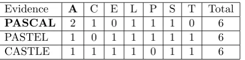
the journal Practical Activities. Suppose that we have three dice and that we paste the letters of the following words on each die, one letter per side: pascal, pastel, and castle.
Suppose then, that we place all three dice in a bag. What is the probability that we select
the die who’s letters spelled out the word “pascal”? Furthermore, suppose we select one
of the die from the bag without looking and roll it on a table. What is the probability
that we chose the “pascal” die given that we rolled an A, that is,P(pascal|A)? To answer
this question we first create a table with the sample space. See Table 2.1. Anyone with
a background in probability can see that this is a straight forward answer. If we see an
“A” the odds are 2 : 2 in favor of “pascal” because it has 2 A’s out of the 4 total A’s,
P(pascal|A) = 2
2 + 2 =
2
4 =
1 2.
Evidence A C E L P S T Total
PASCAL 2 1 0 1 1 1 0 6
PASTEL 1 0 1 1 1 1 1 6
CASTLE 1 1 1 1 0 1 1 6
Table 2.1: Sample space for the “pascal,” “pastel,” and “castle” dice.
However, lets answer the same question using Bayes’ rule. Since Bayesian
statis-tics requires that we use our prior belief about a phenomenon to determine the probability
of some occurrence, we must assign a probability to our prior belief that we have selected
also need to ask the question, “What is the probability that we get an “A” given that we
rolled the “pascal” die?” Since there are 2 A’s out of 6 letters this is
P(A|pascal) = 2
6 =
1 3.
We now apply Bayes’ rule,
P(pascal|A) = P(A|pascal)P(pascal)
P(A|pascal)P(pascal) +P(A|pastel)P(pastel) +P(A|castle)P(castle)
P(pascal|A) =
1 3 × 1 3 1 3 × 1 3 + 1 6 × 1 3 + 1 6 × 1 3
P(pascal|A) =
1 9 1 9+ 1 18+ 1 18
P(pascal|A) =
1 9 4 18 = 1 2.
As expected, we got the same answer as in the straight forward case. The probability of
selecting the “pascal” die given that we rolled an “A” is 12.
Lets suppose, however, that your prior belief of selecting the “pascal” die is 12. In fact, since the prior is a probability distribution and must add up to 1, we assign the
following priors to the remaining dice, P(pastel) = 16 andP(castle) = 13.Using the same sample space as before we apply Bayes’ rule with the new priors
P(pascal|A) =
1 3 × 1 2 1 3 × 1 2 + 1 6 × 1 6 + 1 6 × 1 3
P(pascal|A) =
1 6 1 6+ 1 36+ 1 18
P(pascal|A) =
1 6 9 36 = 2 3.
Since our prior believe was in favor of the “pascal” die, this yield a higher
posterior probability. If instead we chose 16 as a prior, we get a posterior of 27. As we can see the posterior is affected by our initial choice in prior.
As we learn from our data, we can use our knowledge from the posterior to
2.3
Making Inferences with Bayes
In statistics we use data to make inferences about some unknown parameters.
Since it is usually not possible to gather information from everyone in our population of
interest, we do so from a subset of the population called the sample. We then use the
statistics of the sample to make inferences about the population parameters. In Bayesian statistics these unknown parameters are considered variant, that is, not fixed. Here we
will use θ to denote a single parameter or a collection of parameters, i.e. a vector, and
Θ to represent the parameter space, which is the set of all possible parameter values,
thus, θ ∈ Θ [Hof09]. We will let Y = (y1, y2, . . . yn) represent the data set, which is
treated as a random vector, and Y be the sample space, which is the set of all possible
data sets [Hof09]. In the Bayesian approach we are interested in finding the posterior
distribution, P(θ|Y)—the true value of the unknown parameter θ given the observed dataset Y. To find the posterior distribution we calculate the joint distribution of the
prior and the likelihood. The prior distribution, P(θ), describes our belief about θ, and the likelihood distribution,P(Y|θ), describes our belief about Y if we knewθ to be true [Hof09]. Therefore, if we ignore the scaling constant, the posterior distribution is
P(θ|Y)∝P(θ)P(Y|θ).
The posterior distribution is a summary of our beliefs about the parameter(s) given the
data, which we can represent as a probability distribution with the range of values that
we believe captures the true parameter(s).
In the Bayes’ Rule section, we described Bayes’ rule for discrete data. When
dealing with continuous data, the formula has an integral in the denominator,
P(θ|Y) = R P(Y|θ)P(θ) P(Y|θ)P(θ)dθ.
From here on, we will be speaking in terms of continuous data. The definitions in this
section are taken from A First Course in Bayesian Statistical Methods by Hoff and
In-troduction to Bayesian Statistics by Bolstad.
In Bayesian statistics there are different distributions that we can use to
repre-sent our parameters. In order to make calculations easy, we use a prior distribution that
Definition 2.5. A class P of prior distributions for θis called conjugate for a sampling model p(y|θ) if
p(θ)∈ P ⇒p(θ|y)∈ P.
The distribution that we use for the prior depends on our data. For example,
for count data we can use a Poisson distribution. Other types of distributions include
the Beta, Gamma, Normal, Exponential, and Chi-square distributions. Once we have the
posterior distribution for our data we can use a point estimate for our parameterθ. The point estimate can be the median, mean, or mode of our posterior distribution.
In Bayesian statistics we use a Bayesian interval estimate know as a credible
interval.
Definition 2.6. For0< α <1, a 100(1−α)% credible set forθ is a subset C⊂Θ such that P{C|X =x}= 1−α.
The credible interval summarizes the range of possible values for our
parame-ter(s). We can further restrict this range by selecting the highest posterior density (HPD)
region.
Definition 2.7. (HPD region) A 100×(1−α)% HPD region consists of a subset of the parameter space, s(y)⊂Θsuch that
1. Pr(θ∈s(y)|Y =y) = 1−α;
2. Ifθa∈s(y),and θb∈/ s(y),then p(θa|Y =y)> p(θb|Y =y).
As already mentioned, there are different distributions that can be used to do
a Bayesian analysis. In this section we will illustrate how Bayesian statistical techniques
can be applied using a beta distribution. We start by describing the beta distribution in
terms of Bayesian statistics.
Let X ={xi} for i= 1,2, ...n be a sample data set. The Xi’s are independent
Bernoulli, so x= 0 or 1. We let p represent the proportion of individuals with a certain
characteristic. Then p∼Beta(α, β), where f(p) is the prior distribution,
f(p) = Γ(α+β) Γ(α)Γ(β)p
α−1(1−p)β−1,0≤p≤1;α >0, β >0.
E(p) = α
α+β and var(p) =
αβ
(α+β)2(α+β+ 1),respectively.
Examples of beta prior distributions that are conjugate to the binomial
distri-bution are given in Figure 2.1. The distridistri-bution on the left are symmetric, while those
on the right are skewed. The Beta(1,1) distribution, in the upper left hand corner, is an
example of a non-informative prior, also known as a uniform prior; and the Beta(2,3), in
the upper right hand corner, is an example of an informative prior.
0.0 0.2 0.4 0.6 0.8 1.0
0.6 0.8 1.0 1.2 1.4 Beta(1,1)
0.0 0.2 0.4 0.6 0.8 1.0
0.0
0.5
1.0
1.5
Beta(2,3)
0.0 0.2 0.4 0.6 0.8 1.0
0.0
0.5
1.0
1.5
Beta(3,3)
0.0 0.2 0.4 0.6 0.8 1.0
0 5 10 15 20 Beta(.5,3)
0.0 0.2 0.4 0.6 0.8 1.0
1 2 3 4 5 6 7 Beta(.5,.5)
0.0 0.2 0.4 0.6 0.8 1.0
0.0 0.5 1.0 1.5 2.0 2.5 3.0 Beta(3,1)
Figure 2.1: Plots of beta prior distributions.
The likelihood function is given by the binomial distribution (as a function ofr)
L(p) =f(x|p) =
n
r
pr(1−p)(n
−r),
wherer =Pn
failures in the sample. Also,
n
r
=
n!
r!(n−r)!.
By Bayes’ rule, the posterior is the beta distribution
f(p|X) = Γ(α+β+n) Γ(α+r)Γ(β+n−r)p
α+r−1(1−p)β+(n−r)−1.
The mean and variance for the posterior is given by
E(p|X) = α+r
α+β+n and var(p|X) =
(α+r)(β+n−r)
(α+β+n)2(α+β+n+ 1),respectively.
Recall, that we can ignore the normalizing constant, so the posterior can be
simplified to
f(p|X)∝pα+r−1(1−p)β+(n−r)−1.
Example 2.3.1. Suppose we are interested in knowing the proportion of adults in the
United States that have diabetes. Say we believe that 20% of the adult population has
diabetes, p =.2. We will use data from the U.S. National Center for Health Statistics
(NCHS) from their “simple random sample of the American population” collected between
2009 and 2012. The data was gathered using the American National Health and Nutrition
Examination survey (NHANES), seehttps://www.cdc.gov/nchs/data/series/sr_02/
sr02_162.pdf for more information on the survey. Furthermore, we will use the free software R, which is a language and environment for statistical computing and graphics,
and the LearnBayes library package to analyze the data for this example.
Since we are using a beta distribution we must select our parameters for the
prior to reflect our chosen prior p. Let α = 10.81 and β = 42.24, which were specifically
chosen to produced our desired prior mean of 0.2. We now use the program R to construct
a beta density for the prior and the posterior. We first drew a random sample ofn= 100
from the NHANES data consisting of only adults, see Table 2.2 below. Note that r = 7
and (n−r) = 93.
Diabetes Response
Yes 7
No 93
The beta prior together with the likelihood function yield the posterior
param-eters, α = 17.81 and β = 135.24. Figure 2.2 shows a plot of the prior f(p), likelihood
L(p), and posterior distributions f(p|X) for our data. Here we can see that the mean of
the prior is set at 0.2, while the mean of the likelihood and posterior are 0.09 and 0.12,
respectively.
0.0 0.2 0.4 0.6 0.8 1.0
0
5
10
15
Diabetes
Density
Prior Likelihood Posterior
Figure 2.2: Prior, likelihood, and posterior densities for U.S. adults with diabetes.
The 95% posterior credible interval estimate for p is (0.07,0.17). Since the
posterior mean lies within this interval, we can be 95% confident that the posterior
distribution captures the true mean. Therefore, it is very likely that the percentage of
the adult U.S. population with diabetes is 12%.
It is important to discuss the effect, or lack of, that the prior has on the data.
In this example, we can see that the posterior distribution is heavily influenced by the
likelihood and not so much by the prior. Thus, the data is more informative than the
prior. This shows that regardless of our initial chosen prior, the likelihood will have more
pull on the posterior. As we add more data and use the posterior as the new prior, the
mean of the new posterior should start to resemble the mean of the prior. Therefore, we
should not worry about our initial chosen prior since the posterior is going to be more
2.4
Frequentist vs. Bayesians
It is not worth describing Bayesian statistical techniques without making a
com-parison between this Bayesian paradigm and the frequentist paradigm. As we mentioned
in the history section, the frequentist approached overshadowed the Bayesian approach
during the first part of the 1900’s, and it wasn’t until after the 1950’s that thanks to the
efforts of a few Bayesian statisticians it slowly become accepted in the statistical
commu-nity. Like with any paradigm it has its criticisms, but it also has some clear advantages
over the more traditional frequentist paradigm. In this section we will describe the
fre-quentist and Bayesian paradigms, discuss the advantages of using Bayesian techniques,
and mention some of the criticisms against the Bayesian approach.
We first discuss the frequentist approach to inferential statistics. In this paradigm
parameters about the population are considered to be fixed and unknown; and the
hy-pothesis made about these parameters are either supported or rejected by the data.
Usually, this data comes from a sample of the population. Theoretically, as an infinite
number of samples are drawn from the population, we can construct a relative frequency
distribution, called the sampling distribution, which is used to make estimates about the
population parameters. Thus, we are making estimates based on hypothetical repetitions
of the experiment taken an infinite number of times. These estimates can be made in
terms of probabilistic statements like proportions and confidence intervals. Each time
that we construct a confidence interval we can be certain to some degree that we have
captured the true parameter, however, there is always some chance that we have not
captured the true parameter. When testing a hypothesis, frequentist compare a p-value
to some level of significance in order to reject or “fail to reject” the null hypothesis, H0,
as compared to the alternate hypothesis, H1. A p-value gives the probability of obtaining
the observed value under the assumption that the H0 is true [Ver05]. If the p-value of
our observed test statistic is less than the level of significance we accept the H1, and if
it is equal to or larger than the level of significance, we fail to reject the H0. This
hy-pothesis testing technique, however, leads to Type I and Type II errors. A Type I error
occurs when we rejectH0 when it should have been accepted, and a Type II error occurs
when we acceptH0when it should have been rejected. The frequentist approach requires
an understanding of several concepts that can often be confusing (like, what exactly do
confi-dence intervals, p-values, and most hypothesis test are fairly simple, which is one of the
reasons why prior to the 1920’s the frequentist approach was preferred over the Bayesian
approach.
In the Bayesian paradigm parameters are considered to be unknown random
variables, that is, not fixed. We can also make subjective statements about what we
believe the parameters to be before observing the data. These statements are made
in terms of “degree of believe,”—the personal relative weights that we attach to every
possible parameter value [Bol07]. We can attach different weights to our parameters, all
in a single analysis. These wights are given as a probability distribution, which we already
know is called the prior distribution. Recall that we then combine this prior distribution
with the conditional observed data, that is, the data given the parameter, to obtain the
posterior distribution. For large data sets this can become a very complicated process
if done by hand, but thanks to today’s sophisticated computer software all of this work
can be done for us. The posterior distribution then gives the relative weights that we
attach to each parameter value after analyzing the data [Bol07]. We then construct a
credible interval around the estimated parameter, which indicates with some degree of
confidence that our parameter lies within this interval. Thus, we are directly applying
probabilities to the posterior distribution. Also, as new data comes in, we update our
beliefs about the population parameters by using the posterior as the new prior. It is this
straight forward interpretation of credible intervals, the ability to analyze large data sets,
the ease of adding new data to our analyzes without having to start from the beginning
that makes the Bayesian approach appealing to statisticians.
There are also advantages to using the Bayesian approach over the frequentist
approach. First, as already mentioned, in the Bayesian approach we can directly make
probabilistic statements about the parameters via credible intervals. Recall that credible
intervals indicate how confident we are that we captured the true parameter(s). Therefore,
we can say, “I am 95% confident that my parameter lies within this interval.” In the
frequentist approach, on the other hand, we can only make probabilistic statements about
the unknown parameters through the sampling distribution via confidence intervals, which
only indicate whether or not we have captured the true parameters. With a p-value of
0.05, 95% of our intervals will trap the true parameter, but 5% of the intervals will not.
why these intervals come with the possibility of a Type I or Type II error. Secondly,
Bayesians construct probabilistic distributions using the data that did occur to make
inferences about the population parameters, not on hypothetical random samples that
could have occurred. Thirdly, data doesn’t depend on the experimental set up. We do not
need to specify the number of trials needed for our experiment before collecting data. In
the frequentist approach, data is based on a prespecified experimental set up that depend
on a specific number of trials. Even though there are clear advantages to using Bayesian
statistical methods, it is not free of criticism.
There are two main criticisms to the Bayesian approach that we discuss here,
the use of priors and the intensive calculations required to carry out its analysis. Priors
are criticized because they are subjective and they can vary from researcher to researcher.
However, it is the use of priors that makes Bayesian statistics a powerful tool for data
analysis. It was because of the ability to use different priors that AF 447 was found within
a week of using Bayesian statistical techniques. Bayesian analyses are also criticized
because they are harder to compute due to having to integrate over many parameters.
However, due to the advancement of technology, we now have sophisticated computer
software that can handle the complicated computations involved in analyzing large data.
The frequentist and Bayesian paradigms clearly have some distinctions, with
the first relying on priors and the second on relative frequencies; however, the advantages
of the Bayesian approach makes it a good addition to statistical inference. Determining
which approach is best to use depends both on the type of data being observed and
on the researcher. There are criticism against the Bayesian approach, but there are
characteristics about this approach that makes it easier to work with. For one, credible
intervals are easier to interpret than confidence intervals; it is easier to update our beliefs
as new data comes in, than to have to re do the analyses; and it is more logical to analyze
data that did occur, than to analyze hypothetical data that did not occur. It took years
to develop Bayesian statistical methods and to get statistician on board, but today it
Chapter 3
Linear Regression
3.1
Frequentist Regression
A common interest in statistics is to compare two variables to determine if
there is a relationship. Usually, one variable is known, say x and the other isn’t, say
y. We call X = x1, x2, . . . , xn the predictor variable or the independent variable, and
Y = y1, y2, . . . , yn the response variable or the dependent variable [Ver05]. We usually have n pair of observations (x1, y1),(x2, y2), . . . ,(xn, yn) where X is used to predict Y for a given x, E(Y|x). The method used by the frequentist to estimate the mean of Y
is linear regression. Mathematically, the linear regression model is of the form α+βx,
where the parametersα andβ are linear [HT77]. Without making some assumptions the
simple linear regression model can only be used to analyze bivariate data. In order to
make inferences we need the following assumptions taken from Introduction to Bayesian
Statistics by Bolstad:
1. Mean assumption. The conditional mean ofygivenxis an unknown linear function of x.
µy|µ=α0+βx,
whereβ is the unknown slope andα0 is the unknown y intercept of the vertical line
x= 0. In the alternate parameterization we have
µy|µ=αx¯+β(x−x¯),
x = ¯x. In this parameterization the least squares estimates αx¯ = ¯y and β will
be independent under our assumptions, so the likelihood will factor into a part
depending on αx¯ and a part depending on β.
2. Error assumption. Observation equals mean plus error, which is normally dis-tributed with mean 0 and known varianceσ2. All errors have equal variance. 3. Independence assumption. The errors for all of the observations are independent of
each other.
Therefore, to predict the value ofE(Y|x) we need to take into account the error
associated with each value of X in predicting the mean ofY. To account for this error
we include it in thesimple linear regression model,
Y =α0+βX+i,fori= 1,2, . . . n,
whereα0 and β are theregression coefficients and is N(0, σ2).
Estimating the values for the regression coefficients ˆα0and ˆβgives the estimated
regression line, also known as theprediction line [Ver05]. We use prediction line to make future predictions about the values ofY. In this case, the error term is called the residual,
=yi−yˆi. Thus, the prediction line is
ˆ
Y = ˆα0+ ˆβX.
To estimate ˆα0, ˆβ and ˆσ2 we use maximum likelihood estimates. We find the
maximum likelihood estimates through themethod of least squares, which involves taking the sum of the squared vertical distance between each point (xi, yi) fori= 1,2, . . . , nand
the lineY =α0+βX. The sum of the squares of those distances is given by
H(αx¯, β) =
n X
i=1
[yi−αx¯−β(xi−x¯)]2.
We pick the values forα¯x andβ to be those that minimize the square distances so that we can fit a straight line through our data [HT77]. Thus, ˆα0 = ˆαx¯+ ˆβx¯and ˆβ are
ˆ
αx¯ = ¯y, ˆβ=
n P
i=1
yi(xi−x¯)
n P
i=1
(xi−x¯)2
and ˆσ2 = 1
n n P
i=1
[Y −αˆx¯−βˆ(xi−x¯)]2.
Note that the difference between Y −Yˆ is the residual i = Y −Yˆ, which is
equal to
Y −Yˆ = n P
i=1
[Y −αˆx¯−βˆ(xi−x¯)]2.
Also note that the sum of this difference will be zero or, due to rounding error,
close to zero.
We can rewrite the sum of the squares of the residuals as
SSyy = n X
i=1
[Y −( ˆα¯x+ ˆβ(xi−x¯)]2.
Furthermore, we can construct confidence interval for the point estimates by
using a Student’s t critical value:
ˆ
αx¯±tγ
2 ×SE( ˆα) and ˆβ±t
γ
2 ×SE( ˆβ),
whereγis the confidence level. [HT77].
3.2
Frequentist Regression Example
In this section we will present a simple linear regression example using the
frequentist approach. The data comes from NCHS and was gathered using the NHANES
questionnaire. The variables of interest are “HomeRooms” and “Poverty”. The data was
analyzed using the software R.
Suppose we are interested in knowing if there is a relationship between poverty
level and the number of rooms in the residing household. Thus, we let Poverty be the
predictor variable and HomeRooms be the response variable. According to the NHANES
R document, Poverty is defined as “a ratio of family income to poverty guidelines,”
where “smaller numbers indicate more poverty.” Please see the U.S Department of Health
and Human Services web page for the 2009 through 2012 poverty guide lines for all
2009-hhs-poverty-guidelines. Also, HomeRooms is defined as “[the number of] rooms [that] are in the home of [the] study participant (counting kitchen but not bathroom)”
where “13 = 13 or more rooms.” A sample of n= 500 U.S. adults with no replacement
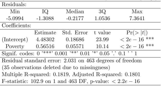
was used. After running the data through R and using it’s built in linear model function
lm() for basic frequentist linear regression, we obtained the following output, see Table
3.1.
Call: lm(formula = HomeRooms ∼Poverty, data = sampleage)
Residuals:
Min IQ Median 3Q Max
-5.0994 -1.3088 -0.2177 1.0536 7.3641
Coefficients:
Estimate Std. Error t value Pr(>|t|)
(Intercept) 4.48302 0.18686 23.99 <2e−16 ***
Poverty 0.56516 0.05571 10.14 <2e−16 ***
Signif. codes: 0 ’***’ 0.001 ’**’ 0.01 ’*’ 0.05 ’.’ 0.1 ’ ’ 1 Residual standard error: 2.031 on 463 degrees of freedom (35 observations deleted due to missingness)
Multiple R-squared: 0.1819, Adjusted R-squared: 0.1801 F-statistic: 102.9 on 1 and 463 DF, p-value: <2.2e−16
Table 3.1: Frequentist linear regression R output.
The point estimates for the regression coefficients are ˆα = 4.48 and ˆβ = 0.57,
with the following respective 95% confidence intervals (4.12,4.85) and (0.46,0.67). In this
traditional approach we can be confident that 95% of th time our intervals will capture
the true parameters. Thus, the prediction line is
5 10
0 1 2 3 4 5
Poverty Level
Number of Home Rooms
Figure 3.1: Relationship between “Poverty Level” and “Number of Home Rooms” in the
frequentist model.
In Figure 3.1 we can see that there is a positive linear relationship between
poverty level and number of home rooms. The results are not surprising, we would expect
that as poverty level goes up, so does the number of rooms in the residing household. In
the next section we will present the same example, but from a Bayesian approach.
3.3
Bayesian Regression
There are some similarities between the frequentists’ regression and the Bayesians’
regression, except for some obvious differences like the use of priors and updating
func-tions in the Bayesian approach. Recall that in general Bayes’ rule is given by
posterior∝prior×likelihood.
Furthermore, since the Bayesian approach makes use of conjugate priors, we first
deter-mine the distribution for the likelihood function and then decide on the prior for the
model.
In the Bayesian approach, data is considered fix, therefore, in simple Bayesian
likelihood of all the observations as a function of the parameters αx¯ =α and β is given
as a product of the individual likelihoods, which are all independent, thus we have,
f(yi|α, β)∝ n Y
i=1
e−2σ12[yi−(α+β(xi−¯x))]
2
.
Since this product can be found by summing the exponents, we can rewrite it as
f(yi|α, β)∝e−
1 2σ2
Pn
i=1[yi−(α+β(xi−x¯))]2. Then β ∼ N(B,SSxxσ2 ), where B = SxySxx =
Pn
i=1(xi−x¯)(yi−y¯) Pn
i=1(xi−¯x)2 and SSxx =
Pn
i=1(xi −x¯)2, and α∼N(Ax¯,σ
2
n), whereAx¯= ¯y.
Since the likelihood has a normal distribution we can chose the normal
distri-bution for the prior or a non-informative prior like the uniform distridistri-bution. If we select
a uniform prior, the prior will be equal to 1; however, if we select normal priors, this will
be
g(α, β) =g(α)×g(β)∝e−
1
s2α(µ−mα)×e
−1
s2 β
(µ−mβ)
,
where α ∼ N(mα, s2α) and β ∼ N(mβ, s2β). Note that to find the variances s2α and s2β
we pick a possible upper and lower bound for y, take their difference, and divide by 6
[Bol07]. Using Bayes’ rule, the posterior is
g(α, β|yi)∝g(α, β)f(yi|α, β).
Then α ∼ N(m0α,(s0α)2) and β ∼ N(m0β,(s0β)2). Since we use a prior conjugate to the posterior, then as new observations are made we can use the updating functions to find
the mean and variance for the new posterior. Thus, for α∼N(m0α,(s0α)2) we have 1
(s0
α)2
= 1
s2
α
+ n
σ2
for the posterior precision, which is the reciprocal of the variance, and the posterior mean
m0α=
1
s2
α
1 (s0
α)2
×mα+ n σ2
1 (s0
α)2
×A¯x.
Also, for β ∼N(m0β,(s0β)2) we get 1 (s0β)2 =
1
s2
β
+SSx
and
m0β =
1
s2
β
1 (s0
β)2
×mβ+ SSx
σ2
1 (s0
β)2
×B,
for posterior precision and posterior mean, respectively.
Recall that the posterior distribution summarizes our belief for the parameter’s
true value. In Bayesian statistics we can construct a credible interval to describe the range
of possible parameters, which captures this true value. In Bayesian linear regression, we
can construct a credible interval for both the intercept, here at x = ¯x, and the slope β.
When σ2 is unknown, which it usually isn’t, we use the estimated population variance ˆσ2
calculated from the residuals
ˆ
σ2=
Pn
i=1(yi−(Ax¯+B(xi−x¯)))2
n−2 .
The credible interval will be
m0β±zγ
2 ×
q
(σ0β)2.
However, to account for the unknown σ2 we can widen our credible interval and use a
Student’s t critical value instead of the normal critical value z. In this case, we use
m0β±tγ
2 ×
q
(s0β)2
[Bol07].
3.4
Bayesian Regression Examples
Here we present a simple Bayesian linear regression example using the NHANES
data. Our variables of interest are the same as in the previous section, “HomeRooms”
and “Poverty”. In order to make a comparison between the frequentist approach and the
Bayesian approach, we will be asking the same question as before, “Is there a relationship
between poverty level and the number of home rooms in the residing household?”. Again,
we analyze the data using the software R. However, this time we use the library package
MCMCglmm for Bayesian linear regression analyses. We will present two models, the
first using a non-informative prior and the second using an informative, also known as
subjective, prior. In each case we use a sample size of n = 500 of U.S. adults with no
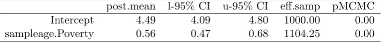
Example 3.4.1. In the non-informative prior model, we select a uniform prior
distribu-tion. This means that we give each parameter an equal probability of occurrence, thus,
α= 0.5 and β = 0.5. After running the model we obtain the output in Table 3.2.
post.mean l-95% CI u-95% CI eff.samp pMCMC
Intercept 4.49 4.09 4.80 1000.00 0.00
sampleage.Poverty 0.56 0.47 0.68 1104.25 0.00
Table 3.2: Bayesian linear regression R output with non-informative prior.
The point estimates for the Bayesian regression coefficients are ˆα= 4.49, with
credible interval (4.09,4.80), and ˆβ = 0.56, with credible interval (0.47,0.68). These
estimates closely resemble the point estimates from the frequentist linear regression model.
This is to be expected since we used a non-informative prior, so the model from both
approaches should be similar. The Bayesian model here is
HomeRooms= 4.49 + 0.56P overty.
However, the credible intervals are interpreted differently. Here we are saying that we are
95% confident that our intervals contain the parameters.
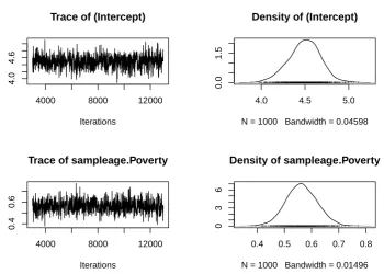
In Bayesian statistics we can also run diagnostics on our models, in the form
of a trace plot and a density plot. A trace plot shows the history of a parameter value
across iterations of the chain along the x-axis, while a density plot shows the distribution
of the data. Figure 3.2 shows the trace plot for the intercept and Poverty. As we can see,
the trace for the intercept and for Poverty have a caterpillar shape, which means that the
iterations were consistent throughout the chain. Also, the density plots show a normal
distribution around the parameter estimates. Thus, we can be fairly confident that we
4000 8000 12000
4.0
4.6
Iterations
Trace of (Intercept)
4.0 4.5 5.0
0.0
1.5
Density of (Intercept)
N = 1000 Bandwidth = 0.04598
4000 8000 12000
0.4
0.6
Iterations
Trace of sampleage.Poverty
0.4 0.5 0.6 0.7 0.8
0
3
6
Density of sampleage.Poverty
N = 1000 Bandwidth = 0.01496
Figure 3.2: Trace and density plots for Intercept and Poverty for the Bayesian model
with non-informative prior.
The positive linear relationship between poverty level and the number of home
rooms in the residing household is presented in Figure 3.3. Again, as the poverty level
increases so does the number of rooms in the residing household. Recall that lower values
5 10
0 1 2 3 4 5
Poverty Level
Number of Home Rooms
Figure 3.3: Relationship between “Poverty Level” and “Number of Home Rooms” in the
Bayesian model with non-informative prior.
The Bayesian approach using a non-informative prior yield a similar model using
the frequentist approach. However, with the Bayesian approach it is simpler to interpret
the credible intervals, and as we gather more data we are able to add it to our model by
making the posterior distribution our new prior distribution.
Example 3.4.2. Here we present the Bayesian linear regression model with an
informa-tive priors α= 6 and β= 1, and variance σ2= 0.02. See Table 3.3 for the R output.
post.mean l-95% CI u-95% CI eff.samp pMCMC
Intercept 5.55 5.39 5.73 388.84 0.00
sampleage.Poverty 0.35 0.28 0.42 893.21 0.00
Table 3.3: Bayesian linear regression R output with informative prior.
The estimated regression coefficients for the model are ˆα = 5.55 and ˆβ =
0.35 with corresponding critical intervals (5.39,5.73) and (0.28,0.42), respectively. The
Bayesian linear regression model is
In this case, since we used an informative prior, the posterior distribution was
more heavily influenced by the prior than by the data. Notice that our estimated alpha
value, ˆa= 5.55, closely resembles the alpha in our chosen prior,α= 6. This yield a higher
value compared to when we chose a non-informative prior in the previous example.
In Figure 3.4 we can see the trace and density plots for the intercept and for
Poverty. Again we see a caterpillar shape for the trace and a normal distribution for the
density. Therefore, we can again be confident in our model.
4000 8000 12000
5.3
5.6
Iterations
Trace of (Intercept)
5.3 5.4 5.5 5.6 5.7 5.8 5.9
0
2
4
Density of (Intercept)
N = 1000 Bandwidth = 0.02287
4000 8000 12000
0.25
0.40
Iterations
Trace of sampleage.Poverty
0.25 0.30 0.35 0.40 0.45
0
4
8
12
Density of sampleage.Poverty
N = 1000 Bandwidth = 0.009066
Figure 3.4: Trace and density plots for Intercept and Poverty for the Bayesian model
with informative prior.
In Figure 3.5 we see the positive relationship between both of our variables, as
5 10
0 1 2 3 4 5
Poverty Level
Number of Home Rooms
Figure 3.5: Relationship between “Poverty Level” and “Number of Home Rooms” in the
Bayesian model with informative prior.
In this chapter we saw three simple linear regression models. One from the
frequentist perspective and two from the Bayesian perspective. In the next chapter we
Chapter 4
Hierarchical Linear Regression
4.1
Bayesian Hierarchical Linear Regression
When we involve multiple predictor variables, each with different levels, we need
a hierarchical model to account for the multiple parameters. Recall that the Bayesian
model in its proportional form is
posterior∝prior×likelihood.
In Bayesian hierarchical models, each prior has its own distribution with its own
param-eters, which we call hyperparameters. If we let φ represent the hyperparameters and θ
represent the parameters of interest, then p(φ) is the hyperprior distribution and p(θ|φ)
is the likelihood function. Thus, their joint distribution is p(φ, θ) =p(φ)×p(θ|φ). Then
by Bayes rule, in its proportional form, we have
p(φ, θ|y)∝p(φ, θ)p(y|φ, θ),
whereyis a vector of data points, andp(φ, θ|y) is the posterior. Note that the right hand
side can be simplified to p(φ, θ)p(y|θ)–since the hyperparameters φ affect y through θ,
the data only depends on θ.
Next we describe the random effects model (also known as simple varying
coef-ficients model) and the mixed-effects model were the regression coefcoef-ficients are
exchange-able and normally distributed. For these models we use a prior distribution of the form
regression model for the likelihood, y∼N(Xβ,P
y),whereX is the J×J matrix, and
regression coefficients are relabeled as βi fori= 1, . . . , J [GCS+14].
In the random effects model, the β are exchangeable and their distributions
are in the form β ∼ N(1µ, τ2I), where 1 is the J ×1 vector of ones [GCS+14]. This means that we can condition on the indicator variables, which represent subgroups of the
population. Thus, we can have different mean outcomes at each level. In general, the
hierarchical random effects model is,
Yij =βj+ij forij ∼N(0, σ2).
In the mixed-effects model, the firstJ1 components ofβ are assigned an infinite
prior variance and the remaining J2 =J −J1 are exchangeable with a common mean µ
and a standard deviation σ [GCS+14]. We can then write β
j =µ+sj, where µ is the
overall mean and sj is some normal random effect. The mixed-effect model is
Yij =µ+sj+ij forij ∼N(0, σ2),
where µis the fixed effect, sj is the random effects, andij are the individual effects.
Here we discuss a Bayesian generalized linear mixed model (GLM), specifically,
the Poisson regression model. The Poisson model is used for count data with
over-dispersion, that is, for data that has more variation than is expected [Had10]. Note that
the Poisson density function is of the form
P(θ) = 1
θλ
θexp(−λ)
forθ= 0,1,2, . . . with mean and variance
E(θ) =λand var(θ) =λ.
The Poisson model uses a log link function, thus the model is
logY =α+βX
or alternatively,
Y =eα+βX.
In the next section we will present an example of a Bayesian hierarchical Poisson
4.2
Bayesian Hierarchical Linear Regression Example
In this section we present a Bayesian hierarchical Poisson linear regression model.
We will also compare the hierarchical model to a basic linear regression model to show
the effect of adding a random variable. Here we continue to use the NHANES data for
2009-2012. We will use “HomeRooms”, “HHIncomeMid”, and “MaritalStatus” as our
variables. HomeRooms is defined as before. HHIncomeMid is the middle income of the
“total annual gross income for the household in U.S. dollars,” which ranges from 0 to
100,000 or more [Pru15]. MaritalStatus is the marital status of the study participant,
which falls under one of the following categories: Married, Widowed, Divorced, Separated,
NeverMarried, or LivePartner (living with partner)[Pru15]. For all the models in this
section we used a sample of n = 400 U.S. adults with no replacement.
We first present a basic linear regression model using the frequentist approach.
In this model we use HHIncomeMid as the prediction variable and HomeRooms as the
response variable. To analyze our data we use the R software and its built in generalized
linear model function glm(). After running the data we obtained the following output,
see Table 4.1.
glm(formula = HomeRooms ∼HHIncomeMid,
family = poisson, data = sample df): Deviance Residuals:
Min 1Q Median 3Q Max
-2.9824 -0.5523 -0.1070 0.3523 2.8453
Coefficients:
Estimate Std. Error z value Pr(>|z|)
(Intercept) 1.555e+00 4.578e-02 33.960 <2e−16 ***
HHIncomeMid 4.544e-06 6.349e-07 7.158 8.2e-13 ***
Signif. codes: 0 ’***’ 0.001 ’**’ 0.01 ’*’ 0.05 ’.’ 0.1 ’ ’ 1 (Dispersion parameter for poisson family taken to be 1) Null deviance: 322.37 on 399 degrees of freedom
Residual deviance: 270.63 on 398 degrees of freedom AIC: 1730.1
Number of Fisher Scoring iterations: 4
Table 4.1: Frequentist Poisson linear regression R output.
confidence intervals (1.46,1.64) and (0.000003,0.000006), respectively. Thus we have,
logHomeRooms= 1.56 + 0.000005HHIncomeM id
or by exponentiating the coefficients, we have
HomeRooms=e1.56+0.000005HHIncomeM id.
As we can see in Figure 4.1, there is a positive linear relationship between median
income and number of home rooms. As the median income increases there is also a slight
increase in the number of home rooms in the residing household.
5 10
0 25000 50000 75000 100000
Median Income
Number of Home Rooms
Figure 4.1: Relationship between “Median Income” and “Number of Home Rooms” in
the frequentist and Bayesian Poisson models.
The second model that we present here is a basic Bayesian linear regression
model with a Poisson distribution. We look at the relationship of the same variables
as before, “HomeRooms” and “HHIncomeMid”. We use a Poisson regression instead of
ordinary least squares because the response variable (HomeRooms) consists of counts.
We also used the default prior, which consists of a mean of 0 and a variance of 1. Next