A New Legendre Wavelets Decomposition Method for Solving PDEs
Naima Ablaoui-Lahmar,
aOmar Belhamiti
b,∗and Sidi Mohammed Bahri
ca,b,cDepartment of Mathematics and Computer Science, Abdelhamid Ibn Badis University, Mostaganem 27000, Algeria.
Abstract
In this paper, we present a novel technique based on the Legendre wavelets decomposition. The properties of Legendre wavelets are used to reduces the PDEs problem into the solution of ODEs system. To illustrate our results, two examples are studied using a special software package which implements the proposed algo-rithms.
Keywords: Legendre Wavelets, Legendre Polynomials, Operational Matrix of integration, Telegraph Equation.
2000 MSC:49M37, 30E25. c2012 MJM. All rights reserved.
1
Introduction
Since the introduction of Legendre wavelets method (LWM), for the resolution of variational problems, by Rezzaghi and Yousefi in 2000 and 2001 [5, 7], several works applying this method were born. To mention a few, we give : the resolution of differential equations [3, 11, 12], the study of optimal control problem with constraints [6], the resolution of linear integro-differential equations [8], the numerical resolution of Abel equation [10], the resolution of fractional differential equations [2, 4].
The LWM transforms a boundary value problem (BVP) into a system of algebraic equations [5]. The un-known parameter of this system is the vector whose components are the decomposition coefficients of the BVP solution into Legendre wavelets basis.
In this paper, we apply the Legendre wavelets method to solve a partial differential equation, whose un-known function depends on spatial and temporal variables. But the decomposition of this unun-known function into Legendre wavelets basis will be done only on the spatial variable. Obviously, the coefficients of this decomposition will depend on the temporal variable. Hence, via this technique, the solution of a partial dif-ferential equation is reduced to the solution of a time-dependent difdif-ferential equation. As an application of this procedure, we present a numerical simulation of the telegraph equation. This equation modelled several phenomenas in electronics and electricity. It appears in particular during the description of the propagation of the electric signals along a transmission line.
This paper is organized as follows: In section 2, we give a detailed description of the Legendre wavelets
decomposition of a function dependent on the temporal variabletand the space variablex. Section 3 is
de-voted to the operational matrix of integration. In section 4, we apply our technique on the telegraph equation. In section 5, we present formulas of errors calculation. For the last section, the performance of the new method is illustrated with two numerical examples.
2
Decomposition in Legendre wavelets basis
We start this section by recalling that the Legendre wavelets [5] are defined on the interval[0, 1]as follows
: for all j ∈ N∗, n = 1, 2, 3, ..., 2j−1 (the number of levels), m = 0, 1, ...,nc−1 (the order of the Legendre
∗Corresponding author.
E-mail addresses: [email protected] (O. Belhamiti), prof [email protected] (N. Ablaoui-Lahmar), and
polynomials) andncis the number of collocation points ;
ψn,m(x) =
( q
m+122j/2Lm 2jx−2n+1 n2j−1−1 ≤x< 2jn−1
0, otherwise, (2.1)
where Lm(x) are the Legendre polynomials of order m defined on the interval [−1, 1] and satisfy the
following recursive formula:
Lk+1(x) =
2k+1
k+1
xLk(x)−
k k+1
Lk−1(x) (2.2)
withL0(x) =1,L1(x) =xandk=1, 2, 3, ....nc−2.
It is established [3, 5–7] that the family{ψn,m:n≥1 , m≥0}forms an orthonormal basis of the Hilbert
spaceL2([0, 1]), i.e. any elementh∈L2([0, 1])may be expanded as
h(x) =
+∞
∑
n=1+∞
∑
m=0Cn,mψn,m(x), (2.3)
where the approximation coefficients are entirely determined byCn,m = hh,ψn,mi, in whichh., .idenotes the
inner product ofL2([0, 1]).
Since the series (2.3) converges on[0, 1], the functionhcan be approximated as
h(x)' 2j−1
∑
n=1nc−1
∑
m=0Cn,mψn,m(x) =CTΨ(x), (2.4)
whereCandΨ(x)are 2j−1ncvectors given by
C=hC1,0,C1,1, ...,C1,nc−1,C2,0, ...,C2,nc−1, ...,C2j−1,0, ...,C2j−1,nc−1
iT
, (2.5)
and
Ψ(x) =hψ1,0(x), ....,ψ1,nc−1(x), ...,ψ2j−1,0(x), ...,ψ2j−1,nc−1(x)
iT
. (2.6)
Decomposition in an otherL2-space
Let us consider the space
H=L2[0,T];L2([0, 1]), (2.7)
see [1]. We want to give a Legendre wavelets decomposition of an elementhinH:
h: [0,T] → L2([0, 1])
t → h(t, .). (2.8)
As the functionh(t, .)belongs toL2([0, 1]), then by (2.3) we have
h(t,x) =
+∞
∑
n=1+∞
∑
m=0Cn,m(t)ψn,m(x), (2.9)
where the coeficientsCn,m(t)depending on the variabletare defined by
Cn,m(t) =hh(t, .),ψn,mi=
Z 1
0 h(t,x)ψn,m(x)dx. (2.10)
The functions h(t, .)and ψn,m, being both in L2([0, 1]), their product is in L1([0, 1])(according to
Cauchy-Schwartz inequality), which allows us to conclude that the coefficients Cn,m(t) are well defined for allt ∈
[0,T]. Consequently, the relations (2.9) and (2.10) are justified.
For the sequel, we need the following lemmas.
Lemma 2.1. If h∈C [0,T],L2([0, 1])
Proof. It arises from the fact that the inner product is a continuous function of its both arguments.
Lemma 2.2. If h∈C1 ]0,T[,L2([0, 1])
,then the function coefficients Cn,m(t)belong to C1(]0,T[).
Forthermore, if ∂h
∂t ∈L
2 [0,T],L2([0, 1]) ,then
dCn,m(t)
dt =
Z 1
0
∂h(t,x)
∂t ψn,m(x)dx. (2.11)
Proof. Lemma 2.2 is based on
Cn,m(t+∆t)−Cn,m(t)
∆t =
Z 1
0
h(t+∆t,x)−h(t,x)
∆t ψn,m(x)dx,
and
h(t+∆t,x)−h(t,x)
∆t =
∂h
∂t (t,x) +ε(t,∆t,x),
with
lim
∆t→0ε(t,∆t,x) =0.
Lemma 2.3. (Generalization) If h∈Ck ]0,T[,L2([0, 1])
,then the function coefficients Cn,m(t)belong to Ck(]0,T[)
(k≥2).
For allt∈[0,T], the series (2.9) is convergent, we can thus approach any functionhinL2 [0,T];L2([0, 1])
as
h(t,x)' 2j−1
∑
n=1nc−1
∑
m=0Cn,m(t)ψn,m(x) =CT(t)Ψ(x), (2.12)
whereC(t)andΨ(x)are 2j−1nc
functions vectors given by
C(t) =hC1,0(t),C1,1(t), ...,C1,nc−1(t), ...,C2j−1,0(t), ...,C2j−1,nc−1(t)
iT
, (2.13)
and
Ψ(x) =hψ1,0(x), ....,ψ1,nc−1(x), ...,ψ2j−1,0(x), ...,ψ2j−1,nc−1(x)
iT
. (2.14)
3
Operational matrix of integration
In this section, the operational matrix of integration [7] will be obtained. The integration into[0,x], where
x∈]0, 1]of the vectorΨ(x)defined in Eq. (2.14) can be written as
Z x
0 Ψ(t)dt
=PΨ(x), (3.1)
where
P= 1 2j
L F F · · · F 0 L F · · · F
..
. 0 . .. ... ...
F 0 0 · · · 0 L
, (3.2)
is the(2j−1nc)×(2j−1nc)operational matrix of integration,FandLarenc×ncmatrices given by
F=
2 0 · · · 0 0 0 · · · 0
..
. ...
0 0 0
and L=
1 √1
3 0 0 · · · 0 0 0
−√3
3 0
√ 3
3√5 0 · · · 0 0 0
0 −
√ 5 5√3 0
√ 5
5√7 . .. 0 0 0
0 0 −
√ 7
7√5 0 . .. 0 0 0
..
. . .. . .. . .. ... . .. . .. ...
0 0 0 0 . .. −
√ 2nc−3
(2nc−3)√2nc−5 0
√ 2nc−3
(2nc−3)√2nc−1
0 0 0 0 · · · 0
√ 2nc−1
(2nc−1)√2nc−3 0
. (3.4)
4
Application to telegraph equation
The standard form of the telegraph equation is given by
∂2u(x,t) ∂x2 =a
∂2u(x,t) ∂t2 +b
∂u(x,t)
∂t +cu(x,t), (4.1)
with boundary conditions
u(0,t) =α(t) and ∂u(0,t)
∂x =β(t) (4.2)
and initial conditions
u(x, 0) = f(x) and ∂u(x, 0)
∂t =g(x), (4.3)
where
a,b,care constants related respectively to resistance, induction, capacity and conductibility of the cable.
α(t),β(t)are continuous functions in[0,T]and f(x),g(x)are continuous in[0, 1]
We are interested in the evolution of the tensionu(x,t)in a coaxial cable.
Let
∂2u(x,t) ∂x2 =C
T(t)Ψ(x). (4.4)
Integrating (4.4) with respect to second variable over[0,x], we get
∂u(x,t)
∂x =C
T(t)PΨ(x) +
β(t). (4.5)
By a second integration with respect toxinto[0,x], we have
u(x,t) =CT(t)P2Ψ(x) +β(t)x+α(t). (4.6)
As well as
∂u(x,t)
∂t =
dCT(t) dt P
2Ψ(x) + dβ(t)
dt x+ dα(t)
dt (4.7)
∂2u(x,t) ∂t2 =
d2CT(t) dt2 P
2Ψ(x) + d2β(t)
dt2 x+
d2α(t)
dt2 (4.8)
We have also
1=dTΨ(x)
x=eTΨ(x). (4.9)
Substituting (4.4) to (4.9) in (4.1), we obtain
CT(t)Ψ(x) = a(d
2CT(t)
dt2 P
2Ψ(x) +d2β(t)
dt2 e
TΨ(x) + d2α(t)
dt2 d
TΨ(x))
+b
dCT(t) dt P
2Ψ(x) + dβ(t)
dt e
TΨ(x) + dα(t)
dt d
TΨ(x)
+cCT(t)P2Ψ(x) +β(t)eTΨ(x) +α(t)dTΨ(x)
Hence, we have
−aP2TC00(t)−bP2TC0(t) +
I−c P2T
C(t)
= aβ00(t) +bβ0(t) +cβ(t)e+ aα00(t) +bα0(t) +cα(t)d
This system can be solved for unknown coefficients of the vector C(t). Consequently, the solutionu(t,x)
given in (4.6) can be calculated.
5
Error calculation
A reasonable scalar index for the closeness of two functions is the Euclidian norm.
The absolute error for each solution is produced by cumulates of truncation, Legendre Wavelets method and Finite Difference errors. This error is estimated when we know the exact solution by
EA =ku−uek2, (5.1)
whereueis the analytic solution anduis the approximate solution. Also, we consider the pointwise error :
EA,i =|ui−ue(xi)|. (5.2)
6
Numerical results
In this section, we consider two examples to show the efficiency and the accuracy of our method.
6.1
Example 1
Consider in[0, 1]the following boundary values problem
∂2u(x,t) ∂x2 =
∂2u(x,t)
∂t2 , (6.1)
with
u(0,t) =cos(t) and ∂u(0,t)
∂x =0, (6.2)
and
u(x, 0) =cos(x) and ∂u(x, 0)
∂t =0. (6.3)
The exact solution of the problem (6.1)-(6.2) and (6.3) is given by
uex(t,x) =cos(x)cos(t). (6.4)
Suppose that the derivatives onxcan be expressed as
∂2u(x,t) ∂x2 =C
T(t)Ψ(x), (6.5)
∂u(x,t)
∂x =C
T(t)PΨ(x), (6.6)
u(x,t) =CT(t)P2+cos(t)dTΨ(x), (6.7)
then their derivates ontare given by
∂u(x,t)
∂t =
∂CT(t) ∂t P
2−sin(t)dT
Ψ(x), (6.8)
∂2u(x,t) ∂t2 =
∂2CT(t) ∂t2 P
x t
x t
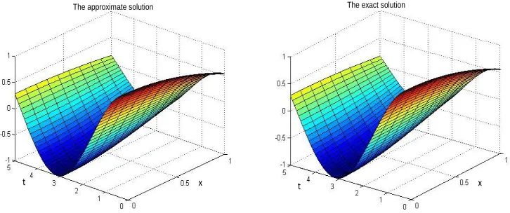
The approximate solution The exact solution
Figure 1: The analytical and approximate solutions.
Substituting (6.5) to (6.9) in (6.1), we obtain
CT(t)Ψ(x) =
∂2CT(t) ∂t2 P
2−cos(t)dT
Ψ(x), (6.10)
and
∂2C(t) ∂t2 −((P
2)T)−1
C(t) = ((P2)T)−1cos(t)d, (6.11) with
CT(0) =eT−dT P2−1 and ∂C(0)
∂t = −→
0 , (6.12)
where
1=dTΨ(x)
cos(x) =eTΨ(x). (6.13)
For the resolution of this problem, we can use a second time the wavelets Legendre method or a finite difference schemes.
We observe a good agreement between the analytical and approximate solutions (see Figure 1). However, the obtained result shows that this technique can provide good performance even when the mesh discretiza-tion has low resoludiscretiza-tion.
We also calculate the absolute error by using formula (5.1), forj=2 andnc=5
EA=1.29e−2. (6.14)
6.2
Example 2
We consider the telegraph equation
∂2u(x,t) ∂x2 =
∂2u(x,t) ∂t2 +4
∂u(x,t)
∂t +4u(x,t), (6.15)
with the conditions
u(0,t) =1+e−2t and ∂u(0,t)
∂x =2, (6.16)
and
u(x, 0) =1+e2x and ∂u(x, 0)
∂t =−2. (6.17)
Suppose that the second derivative ofu(x,t)can be expressed approximately as
∂2u(x,t) ∂x2 =C
Using boundary condition (6.16), we get
∂u(x,t)
∂x =C
T(t)PΨ(x) +2dTΨ(x), (6.19)
u(x,t) =CT(t)P2+2lT+1+e−2tdTΨ(x). (6.20)
We can also express the functions of the right-hand sides of (6.19) and (6.20) as
1=dTΨ(x)
x=lTΨ(x). (6.21)
The derivates ontare given by
∂u(x,t)
∂t =
∂CT(t) ∂t P
2−2e−2tdT
Ψ(x), (6.22)
and
∂2u(x,t) ∂t2 =
∂2CT(t) ∂t2 P
2+4e−2tdTΨ(x). (6.23)
Now by inserting Eqs. (6.18) to (6.23) into equation (6.15), we get
CT(t)Ψ(x) =
∂2CT(t) ∂t2 P
2+4e−2tdT
Ψ(x)
+4
∂CT(t) ∂t P
2−2e−2tdTΨ(x) +
4CT(t)P2+2lT+1+e−2tdTΨ(x).
Thus
∂2C(t) ∂t2 +4
∂C(t)
∂t + (4I−((P
2)T)−1)C(t) =−((P2)T)−1(8l+4d), (6.24)
where
C(0) = ((P2)T)−1(ex−2l−2d) and ∂C(0)
∂t =0, (6.25)
and
1+e2x=exTΨ(x) (6.26)
The exact solution of the problem (6.15)-(6.16) and (6.17) is
uex(t,x) =e2x+e−2t, (6.27)
Applying the same technique as the preceding example, we observe a good agreement between the analytical
and approximate solutions with an absolute errors of order 1.0e−013 (see figure 2). However, the results
obtained show that this technique can provide good performance even when the mesh discretization has low resolution.
We also calculate the absolute error by using formula (5.1), forj=3 andnc=10
EA =1.7705e−013. (6.28)
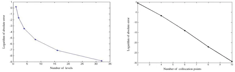
We calculated the absolute error for different values ofjandnc(see figure 3), we observe that :
The effect of the levels number on the solution is shown in Table 1. For j = 1, 2, ..., 6 (2j−1levels), the
absolute errors with respect to analytic solutions are presented. Asjincrease from 1 to 6 fornc=3, the errors
decrease to 10−4.
The considerable effect of collocation points on the solution is shown in Table 2. Fornc =2, 3, ..., 10, the
absolute errors with respect to analytic solutions are presented. As ncchanges from 2 to 4 forj=3, then from
x t
x t
The approximate solution The exact solution
Figure 2: The analytical and approximate solutions.
L
o
g
ar
ith
m
o
f
ab
so
lu
te
er
ro
r
L
o
g
ar
ith
m
o
f
ab
so
lu
te
er
ro
r
Number of levels Number of collocation points
Table 1: Evolution of absolute errors fornc=3
j = 1 j = 2 j = 3 j = 4 j = 5 j = 6
Number of levels 2j-1 1 2 4 8 16 32
Absolute errors 1.2048 1.910E-001 3.1442E-002 5.0610E-003 8.4109E-004 1.43699E-004
Table 2: Evolution of absolute errors forj=3.
nc 2 4 6 8 10
Absolute errors 6.1105e-001 1.1544e-003 7.3398e-007 2.3729e-010 1.7700e-013
7
Conclusion
This work shows that the Legendre wavelets method is a very effective technique for reducing partial differential equations into a set of ordinary differential equations. This numerical method has been tested under different examples. Satisfactory results have been obtained even for a small number of collocation points. The convergence, stability of the solution and accuracy of the results prove the high quality of this method.
8
Acknowledgments
The authors wish to express their sincere thanks to the editor and the reviewer for valuable suggestions that improved the final manuscript.
References
[1] R. Dautray and J.-L. Lions: Mathematical Analysis and Numerical Methods for Science and Technology. Vol. 8: Evolution : semi-groupe, variationnel, ´edition Masson, 1980.
[2] Jafari, S.A. Yousefi, M.A. Firoozjaee, S. Momanic, C.M. Khalique dApplication of Legendre wavelets for solving fractional differential equations, Computers and Mathematics with Applications 62 (2011) 1038– 1045[5]
[3] F. Mohammadi, M.M.Hosseini : A new Legendre wavelet operational matrix of derivative and its appli-cations in solving the singular ordinary differential equations, Journal of the Franklin Institute 348 (2011) 1787–1796
[4] Mujeeb ur Rehman, Rahmat Ali Khan : The Legendre wavelet method for solving fractional differential equations, Commun Nonlinear Sci Numer Simulat 16 (2011) 4163–4173.
[5] Razzaghi M, Yousefi S. : Legendre wavelets direct method for variational problems.Mathematics and Computers in Simulation, 53, 2000, 185-192.
[6] Mohsen Razzaghi and Sohrabali Yousefi : Legendre wavelets method for constrained optimal control problems, Mathematical Methods in the Applied Sciences, 25:529–539, 2002.
[7] Razzaghi M, Yousefi S. The Legendre wavelets operational matrix of integration. International Journal of Systems Science 2001; 32:495–502.
[8] M.Tavassoli Kajani,A.Hadi Vencheh :Solving linear integro-differential equation with Legendre wavelets.International Journal of Computer Mathematics 81, 2004, 719-726.
[10] Sohrab Ali Yousefi : Numerical solution of Abel’s integral equation by using Legendre wavelets, Applied Mathematics and Computation 175 (2006) 574–580.
[11] Xiao-Yang Zheng, Xiao-Fanyang, Young Wu. :Technique for solving differential equation by extended Legendre wavelets.International Conference on wavelet analysis and Pattern Recognition,Hong kong Proceed. , 2008, 30-31.
[12] Xiaoyang Zheng and Xiaofan Yang : Techniques for solving integral and differential equations by Legen-dre wavelets, International Journal of Systems Science Vol. 40, No. 11, November 2009, 1127–1137
Received: October 11, 2013;Accepted: December 21, 2013
UNIVERSITY PRESS