UDC: 551.577.2:519.87
SWAT-Based Runoff Modeling in Complex Catchment Areas –
Theoretical Background and Numerical Procedures
Z. Simić1*, N. Milivojević2, D. Prodanović3, V. Milivojević4, N. Perović5
Institute for Development of Water Resources “Jaroslav Černi”, 80 Jaroslava Černog St., 11226
Beli Potok, Serbia; e-mail: 1[email protected], 2[email protected],
Faculty of Civil Engineering, University of Belgrade, 73 Bulevar Kralja Aleksandra St., 11000
Belgrade, Serbia; e-mail: 3[email protected], 5[email protected]
*Corresponding author
Abstract
This paper shows the structure of the SWAT-based model used in modeling of the “rainfall-runoff” process. The SWAT model is hydro-dynamic and physically-based model for application in complex and large basins. Model inputs are as follows: rainfall, air temperature, soil characteristics, topography, vegetation, hydrogeology and other relevant physical parameters. The model is based on five linear reservoirs as follows: reservoir of the vegetation cover, snow accumulation and melting, surface reservoir, underground reservoir and surface runoff reservoir. The model uses GIS tools for preprocessing and post-processing. The basic modeling unit is the hydrologic response unit (HRU), defined as the network of elementary hydrologic areas with the selected discretization, measure of which is dependent upon the desired accuracy, as well as upon data accuracy. The total runoff on the exit profile of the catchment is computed by convolution of the sum of runoffs (surface and base runoffs). The model can be applied at the daily and hourly level of discretization and used for multiannual simulations. Illustration of operation of the SWAT based model will be presented on a selected
part of the River Drina basin (with the total area of around 20.000 km2).
Keywords: Rainfall-runoff model, linear reservoirs, GIS tools, snow accumulation and melting, potential and real evapotranspiration, total catchment runoff, surface runoff, underground runoff.
1. Introduction
The most important objects of complex management of catchment waters are numerous large multi-user storages capturing the basin inflow for the purpose of water supply to urban areas or irrigation for agricultural areas, flood protection, recreation or electricity generation. As fresh and clean water is becoming scarcer and water pollution by human beings grows, a better distribution of demand coming from a growing number of water consumers is becoming the imperative.
evaluate basin water circulation at the daily, weekly, monthly or annual level. If the evaluations are based on incomplete information, relevant evaluated water discharge in the basin may be fairly incorrect. For example, if the water inflow to storage has been forecasted, advance emptying can be performed so it can to receive potential flood. But, if the emptying in advance is not necessary, then certain water volume would be spilled uselessly (without electricity generation), although it could be precious during the dry seasons.
Water circulation modeling in mathematical model, i.e. hydro-information systems, is not possible without modeling of transformation of rainfall into runoff. Water falls in the form of rain or snow, then the part of it stays on the vegetation, then evapotranspiration and sublimation processes occur, and available water off and forms the river watercourses. These processes are the starting point for modeling of water use for hydropower, management of water resources and other purposes. Present paper describes the use of SWAT model in majority of Serbian hydro-information systems (“Drina” HIS, “Vlasina” HIS and others).
SWAT is the abbreviation for the Soil and Water Assessment Tool model, developed in USDA, (Neitsch et al., 2005). SWAT was designed to make possible the testing and further forecast of water circulation in soil, sediments and farming pesticides and herbicides in large basins with diverse soil and vegetation classes in long time periods. In order to meet these requirements, the model is physically-based and regression equations are used to describe relations between input and output values. SWAT model includes physical patterns which describe the water circulation, sediment circulation, vegetation growth and nutrients circulation by applying required input data on climate, soil characteristics, terrain topography, vegetation topography and land use in the catchment area. SWAT is the continuous time model usable in long-term simulations. The model is not envisaged for simulation of details such as flood wave episodes and similar.
2. Historical development of SWAT model
SWAT model development is an ongoing process, taking place at USDA Agricultural Research
Service (ARS) for almost 30 years now. Current version of the SWAT model is the successor of “the Simulator for Water Resources in Rural Basins” model (SWRRB) (Arnold and Williams, 1987), created to simulate water management and sediment transport in non-investigated (non-gauged) basins in the USA. SWRRB model development started in early 80's in the form of CREAMS, (Arnold et al., 1995b) hydrologic model modification, which was then used to
develop Routing Outputs to Outlet (ROTO) model in early 90's of the last century. This was a
support toll for the management of the underground flow in the basins of Indian countryside in Arizona and New Mexico that covers the area of several thousands of square kilometers. ROTO model development was demanded by the US Bureau of Indian Affairs.
Further important step was the integration of the two models, SWRRB and ROTO, into a single model (SWAT model). SWAT preserved all SWRRB model options, as a very useful simulation model for simulation of processes in very extensive areas.
Then, SWAT model was exposed to constant critique and simultaneous development. Crucial improvements of earlier model versions (SWAT 94.2, 96.2, 98.1, 99.2, and 2000) were described by Arnold and Fohrer (2005) and Neitsch et al. (2005).
catchment into numerous sub-catchments, which are further divided in the elementary hydrologic response units (HRU), the land use, vegetation and soil characteristics of which are homogenous. Multiple HRUs in a single area make a sub-catchment (with clear watersheds and areas), while HRUs are not recognizable space-wise, but they exist only in simulations.
SWAT model uses the following inputs: daily rainfall, the maximum and minimum air temperature, solar radiation, relative air humidity, wind speed. They inputs originate either from the metering stations or they were computed beforehand.
Green-Ampt infiltration method is used for application of daily measured or generated rainfall (Green and Ampt, 1911).
Snowfall is determined on the basis of precipitation and the mean daily air temperatures. The model uses maximum and minimum daily air temperatures for computations.
Application of climate inputs includes the following: (1) up to ten elevation zones are simulated for calculation of rainfall distribution per elevation and/or snowmelt process, (2) climate inputs are adapted to simulation model requirements, and (3) forecast of weather conditions is performed as a new option of the SWAT 2005.
Full hydrologic balance of each HRU includes accumulation and evaporation off the plants, determination of effective rainfall, snowmelt, water exchange between surface runoff and soil layer, water penetration into deeper layers, evapotranspiration, sub-surface flow and underground flow and water accumulation.
Estimation of snow-covered area, snow cover temperature and volume of snowmelt is based on the principles described in Fontaine et al. (2002).
SWAT model includes options for estimation of surface runoff from HRUs, which combine
daily or hourly rainfall and USDA Natural Resources Conservation Service (NRCS) curve
number (CN) method (USDA-NRCS, 2004) or Green-Ampt method. Water retention on plants is computed by the implicit CN method, while explicit water retention is simulated by Green-Ampt method. Water collection in soil and its runoff lag are computed by the techniques of water redistribution between the soil layers.
Sub-surface flow simulation is described in Arnold et al. (2005) for fissured soil classes. SWAT 2005 also offers new options for simulations of water level change in soil on HRUs with seasonal oscillations.
Three methods are used for estimation of potential and real evapotranspiration: Penman-Monteith, Priestly-Taylor and Hargreaves (Hargreaves et al., 1985). Water exchange between the soil and the deeper layers occurs through the sub-surface soil layer. Sub-surface flow is fed by the water not used by plants or water that does not evaporate, which can penetrate to sub-surface reservoirs. Water which penetrates to the deepest reservoirs is considered lost for the system, i.e. it is considered a system output.
3. Model in general
sub-catchment are grouped or organized into the following categories: climate, HRUs, storages/lakes, underground, river network and catchment runoff. Elementary hydrologic response units are mainly of square shape on land within the sub-catchments where the vegetation, soil and land use classes are homogenous.
Regardless of the type of problem being modeled and analyzed by the model, background of the method is the water balance of the catchment area. In order to achieve precise forecast of circulation of the pesticides, sediments or nutrients, hydrologic cycle is simulated by the model which integrates overall water circulation in the catchment area. Hydrologic simulations in the catchment area can be divided into two groups. In the soil phase of the hydrologic cycle the processes on the surface and in the sub-surface soil occur, as well as the circulation of sediments, nutrients and pesticides through the water flows in all sub-catchments. In the second phase, the circulation of water and sediment through the river network up to the exit profile are observed.
Hydrologic cycle is simulated by SWAT model, which is based on the following balance equation:
t
t o day surf seep a gw i 1
SW SW (R Q w E Q )
(1)where SWt is the humidity of the soil (mm H2O), SW0 is the base humidity of the soil (mm
H2O), t is time (days), Rday is rainfall volume (mm H2O), Qsurf is the value of surface runoff
(mm H2O), Ea is the value of evapotranspiration (mm H2O), wseep is the value of seepage of
water from soil into deeper layers (mm H2O) and Qgw is the value of underground runoff (mm
H2O).
SWAT model uses the following climate and hydrologic inputs: rainfall, air temperature and solar radiation, wind speed, relative air humidity, snow pack, snowmelt, elevation zones, water volume on plants, infiltration, water seepage into deeper soil layers, evapotranspiration, sub-surface flow, surface flow, lakes, river network, underground flow and other inputs related to vegetation growth and development, erosion on the catchment area, nutrients, pesticides and land use.
3.1. Strengths and limitations of the model
Borah and Bera (2003, 2004) have compared SWAT model with several other models of the
same type. Their 2003 study showed that all models (the Dynamic Watershed Simulation Model
(DWSM) (Borah and Bera, 2004), Hydrologic Simulation Program – Fortran (HSPF)
(Bicknell et al., 1997) and SWAT model) treat the hydrologic processes, sediments circulation and chemical processes applicable in the catchment areas divided into smaller basic sub-catchments. They have concluded that SWAT model is a promising model for long-term simulations, primarily of agricultural basins. They showed in their 2004 study that SWAT and HSPF models can forecast annual volumes of waters and pollution with adequate monthly forecasts, except in months of storms and under unusual hydrologic circumstances (flood waves), when simulation results turn to be considerably worse.
Van Liew and Garbrecht (2003) compared the basin outlet hydrographs produced by SWAT and HSPF models on 8 catchment areas in Little Washita River basin in south-east Oklahoma. The conclusion was that SWAT model is better than HSPF model in terms of runoff forecast for different climate conditions and it may be even better for long-term simulations in the case of the impact of changeable climate factors upon surface water resources.
MIKE-SHE model produced slightly better results. In Srinivasan et al. (2005), it was concluded
that SWAT model gave discharges approximately similar to the ones obtained by the Soil
Moisture Distribution and Routing (SMDR) model (Cornell, 2003) in FD-36 experimental basin in east-central Pennsylvania (total area of 39.5 ha) and that SWAT model can perform good calculations of seasonal changes. In Srivastava et al. (2006), it was determined that the model of
synthetic neural networks (artificial neural network ANN) is better model than SWAT model in
calculation of the runoff from the small basins in south-eastern Pennsylvania.
3.2. Previous model adaptations
SWAT model development was accompanied by numerous modifications, adaptations and improvements of specific processes which were in certain cases focused on specific regions.
The most recent examples are the models SWAT-G, Extended SWAT (ESWAT), and the Soil
and Water Integrated Model (SWIM). The initial SWAT-G model was developed by modification of certain parts of the SWAT 99.2 model, wherein percolation, hydraulic permeability and functions related to water seepage were improved for usual conditions that exist in hill and mountain regions in Germany (Lenhart et al., 2002). ESWAT model (van Griensven and Bauwens, 2003, 2005) brought in several new modifications to the original SWAT model: (1) within-hourly rainfall as inputs and infiltration, discharge and forecast of losses due to the erosion, based on the user time discretization of one hour, (2) water flow through the river network based on one-hour time step and the link with water quality, based on the kinematic wave and functions used in QUAL2E model as additional improvement, (3) multiple (multi-space and/or multi-parameter) calibration and auto-calibration (similar components are built into the SWAT 2005 model). SWIM model is based primarily on hydrologic components of the SWAT model and nutrients circulation from the MATSALU model (Krysanova et al., 1998, 2005) and it was created to simulate processes in the middle
range of basin areas (from 100 to 100.000 km2). The latest SWIM model improvements include
the integration of the dynamic sub-model of underground waters (Hatterman et al., 2004) that increases the capacity of simulation of forest systems (Wattenbach et al., 2005) and develops the use of much more realistic simulations in humid and riparian regions (Hatterman et al., 2006).
3.3. Reasons for development of the new model
As shown here, the SWAT model is complex and applicable under various conditions and for various purposes. It has also been shown that the model had experienced many adaptations and additional developments related to modeling of phenomena in specific basins. After the analysis of the original and numerous adapted models, the Project Team of the Belgrade Institute
“Jaroslav Černi” has decided to perform additional development of SWAT model and its
adaptation to specific basins in the wider area that includes Serbia (Serbia, Montenegro and
Bosnia and Herzegovina) (Prodanović et al., 2009).
4. Theoretical background of the new SWAT model
4.1. Model structure and mathematical background
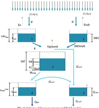
Fig. 1. Scheme of linear reservoirs in SWAT model
First reservoir represents the approximation of the first vertical layer when precipitation is in the form of rain. It represents the layer of vegetation cover of the terrain surface. It is used to simulate water retention on the plant cover.
Second layer also represents the layer above the terrain surface, but when precipitation is in the form of snow. In addition to water retention on plants, in this layer is also simulated water retention in the snow blanket. The outlet of this reservoir is the snowmelt transferred to the following reservoir.
Third reservoir represents the unsaturated soil layer. The inlets of this reservoir are the outlets of the previous two, i.e. effective precipitation and snowmelt. Simulated here is the surface runoff, as well as the seepage to deeper soil layers.
After the soil is saturated and water spilled from the previous reservoir, one part of the water runs to the underground aquifer that the underground or base runoff originates from (fourth reservoir).
Climate inputs are the constants (radiation at the atmosphere boundary and other time constants) and variables (air temperature, rainfall and other) that change in time and space. The elevations of each HRU (obtained by the application of GIS techniques), as well as the areas and other performances, determined for model purposes, are also taken into consideration. Mean rainfall, air temperatures and snow pack height are computed for each HRU.
Mean rainfall
Calculation of referent rainfall values for each HRU by the means of formula (2) is performed because in the case of the sloped terrain the meteorological values change with the change in elevation:
n
laps
k k
HRU gauge HRU gauge R
k 1
p
R R (EL EL ) p
1000
(2)The calculation of referent rainfall values in HRUs is linked to rainfall stations, which are grouped (assigned to sub-catchment) according to the rule of Tiessen polygons (Figure 2).
Fig. 2.
Illustration of the sloped terrain
In Equation (2), Rgaugeis rainfall (mm), EL is elevation (mnm), (ELgauge is the elevation of
the location where the rainfall was recorded (on the rainfall station), ELHRU is the elevation of
the HRU and plaps is the rainfall gradient (mm/km). This is the measure of rainfall growth per
elevation growth and pRkis weight. The following condition is to be met for pRk:
n k R k 1
p 1
(3)where k is the number of rainfall stations which were grouped (assigned to sub-catchment).
Mean Temperatures
performed for mean, minimum and maximum temperatures within the discretization period of calculation:
n
laps
k k
HRU gauge HRU gauge T
k 1
t
T T (EL EL ) p
1000
(4)where T are the minimum, maximum and mean air temperatures, tlaps is the temperature gradient
(oC/km) and pTkis the weight. The following condition is to be met:
n k T k 1
p 1
(5)where k is the number of rainfall stations which were grouped (assigned to sub-catchment).
4.2. Water balance through the unsaturated environment
Hydrologic cycle within a HRU, simulated by this model, is defined by the balance equation (6):
i i 1 i i i i 1 i
melt surf seep t soil
SW SW
(R
SNO ) Q
w
E
(6)where SWiis the water volume in soil in time ti (mm), SWi1the water volume in soil in time
1
i
t (mm), Rithe rainfall volume in discretization period i (mm), i
melt
SNO – water equivalent of
snowmelt (mm), i
surf
Q the volume of surface runoff (mm), i
t soil
E the evapotranspiration of soil
(mm) and i 1
seep
w filtration (water penetration to deeper soil layers) (mm).
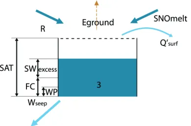
Fig. 3. Reservoir in unsaturated environments (3)
Elements of the Equation (6) are illustrated in Figure 4.
4.3. Snow accumulation and snowmelt
The model separates rainfall into rain and snow depending on the boundary temperature Ts-r. This boundary temperature is not automatically equal to zero degrees of Celsius, but usually it
is either equal or very close to zero (1oC). The snowmelt process is modeled for each HRU
Fig. 4. Balance scheme of SWAT model
Value corresponding to snowmelt is computed according to the following equation:
i i
i i snow max
melt melt cov melt
T T
SNO b sno T
2
(7)
where SNOmelt is the water equivalent of the snowmelt (mm), snocov the snow coverage of the
HRU (%), bmelt the degree-day factor of snowmelt (mm/day oC),Tsnowsnow temperature (oC),
Tmaxthe maximum temperature value recorded during the discretization period (oC) and Tmeltis
the base (referent) temperature of snowmelt (close or equal to zero) (oC). bmelt is computed from
the following expression:
melt 6 melt12 melt 6 melt12
melt n
(b b ) (b b ) 2
b sin( (d 81))
2 2 365
(8)
where bmelt6 is the degree-day factor of snowmelt (mm/day oC) on June 21st of the current year
(mm/day oC), b
melt12 is the degree-day factor of snowmelt on December 21st of the current year
(mm/day oC), d
n is the day of the calendar year (1-365). In years with 366 days, the bmelt value
for December 31st is equal to the value on December 30th.
The following condition is to be met:
i i i
melt sub
0 SNO SNOE (9)
where Esubis the sublimation of water from solid state (snow) to vaporous state, computed only
when T>Tmelt is applicable, according to the following formula:
s sub
sol E E
1 cov
where covsol is the index of vegetation and soil albedo (for snow-pack > 0.5 mm, covsol = 0.5)
and Es is the maximum sublimation (soil evapotranspiration):
s o sol
E E cov (11)
Potential evapotranspiration is computed out of the canopy storage (there are two possible cases):
o o can
E E E , if Eo>Ecan (12)
o o
E E , if Eo<Ecan (13)
where Eo is potential evapotranspiration, Ecan = RINT the value of evaporation of canopy storage
waters and snocov is the part of HRU covered by the snow.
Notion of the spatial curve of reduction of snow pack height is defined as:
1
cov 50cov
100 100 100
SNO SNO SNO
sno exp(1 sno )
SNO SNO SNO
(14)
where SNO100 is the minimum measure of snow pack height for snow coverage of HRU of
100% and sno50cov is the percentage of SNO100 for snow coverage of 50% (the possible range of
values is between 0 and 1).
The following condition is to be met:
snocov≤ 1.0 (15)
Snow temperature is computed according to the following equation:
i i 1 i
snow snow sno dn sno
T T (1 l ) T l (16)
where lsno is the impact of the snow temperature during the previous days and T is the mean dn
daily temperature.
The value of sublimation is computed according to the following equation:
s sub
E E
1.5
(17)
and the following condition is to be met:
dn melt
T T (18)
The maximum sublimation (soil evaporation) Esis the maximum value of sublimation off
the plants during the current day that depends upon canopy storage and is computed as follows:
s o
E E 0.5 (19)
The potential evapotranspiration is computed on the basis of canopy storage (there are two possible cases):
o o int
E E R , if Eo>Rint (20)
o o
E E , if Eo<Rint (21)
where Eo is the potential evapotranspiration (mm) and Rint is the canopy storage (mm). There
i i 1 i i 1 i 1 melt sub
SNO SNO R SNO E , when i
s r
T T (22)
i i-1 i-1 i-1
melt sub
SNO SNO -SNO - E , when i
s r
T T (23)
where SNO is the water equivalent of snow pack height (mm) and SNOmelt is the water
equivalent of the snowmelt (mm). Snow temperature is calculated as follows:
i i 1
snow snow sno dn sno
T T (1 l ) T l (24)
where T is the mean daily air temperature (dn
oC) and i 1
snow
T is the snow temperature for the
previous day.
4.4. Calculation of potential surface runoff
Rainfall value (rain) is computed in the following two ways:
int
R 0, when i
s r
T T (25)
int HRU
R R , when i
s r
T T (26)
In the first case, the rainfall (25) is accumulated as snow and in the second case (26) it is generated as rain. The SWAT model uses SCS CN model for the calculation of the potential surface runoff. There are two potential cases here:
i i 2
i melt
surf i i
melt
(R SNO )
Q
R SNO S
, if SW i-1≥ 0.2
S = Ia (27)i i 2
i melt a
surf i i
melt a
(R SNO I )
Q
R SNO S I
, if SW i-1 < Ia i Ri>Ia (28)
where Ia is the initial condition for surface runoff, R the value of rainfall reaching the soil and S
is the retention parameter calculated from the Equation (29).
1000 25.4 10 S CN
(29)
where CN= f (ITZ, ITV), ITZ the soil type index (generated for each GIS layer) and ITV is the index of the vegetation type (generated for each GIS layer).
4.5. Calculation of potential evapotranspiration (Eo)
Hargreaves method is used for calculation of potential evapotranspiration (this method requires only the mean, minimum and maximum air temperatures):
0.5
o o max min
E 0.0023 H (T T ) (T 17,8)
(30)
where is the latent evaporation heat. Calculation is performed according to the following
equation:
3
2,501 2,361 10 T
(31)In Equation (30) Tmin is the minimum daily temperature (oC), Tmax is the maximum daily
temperature (oC),
T
is the reference temperature in HRU (oC) and Ho is the radiation at the
4.6. Calculation of rainfall reaching soil
The rainfall recorded on rainfall stations (R) does not completely reach the soil if the
vegetation is present that is, one part of rainfall stays on leaves and tree trunks. One part of the rainfall evaporates, while the other part is used by plants. The value of canopy storage is computed using the following two formulas:
Ri
int=Ri-1int+R–Eai-1 and R=0 if: Rcandayi-Ri-1int (32)
Ri
int=candayi and R=R –(candayi-Ri-1int)–Eai-1 if: R>candayi-Ri-1int (33)
where R is rainfall before the plant leaves capture the water, R the rainfall after the plant leaves
capture the water (the rainfall reaching soil (mm)) and Ea is real evapotranspiration (mm). The
following condition is to be met:
int day
R can (34)
Present condition ensures that canopy storage volume is not greater than the maximum water volume which plants can capture on a given day.
The evapotranspiration process includes canopy storage, in fact the part of canopy storage which can have major impact on infiltration, surface runoff and evapotranspiration.
Canopy storage (canday) varies on daily basis and it is the function of plant leaf size. During
the rainfall time, the first condition to meet is the formation of the canopy storage (canday) and
after that the water can reach soil:
day max max LAI can can
LAI
(35)
where canday is the maximum water volume that can stay on plants on a given day, canmax the
maximum water volume that can stay on full-grown plants and LAI (leaf area index) is the total
area of green leaves per ground area on a given day (m2/m2). The following functional
dependency has been created:
LAI=f(LAImax, LAImin, LAI1, LAI2, LAI3, LAI4 ) (36)
where LAImax is the maximum leaf area index per ground area (m2/m2), LAImin the minimum
leaf area index per ground area (m2/m2), LAI
1 the start of the spring vegetation period (day of
the year, for example March 21st), LAI
2 the start of summer vegetation period (day of the year,
for example June 1st), LAI
3 the end of summer vegetation period (day of the year, for example
September 1st) and LAI
4 is the end of the fall vegetation period (day of the year, for example
November 15th). LAI and LAI
max are presented in table form in the database (GIS) for each
vegetation class separately.
4.7. Calculation of real evapotranspiration
After the calculation of potential evapotranspiration and canopy storage water, real (actual) evapotranspiration can be calculated by:
if E0<Rint than Ea=E0 (37)
if RINT=0 than Ea=E0 (38)
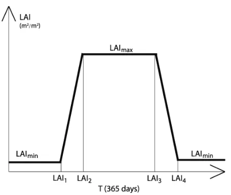
Fig. 5.
Leaf area index per ground area on a given day (m
2/m
2)
4.8. Water penetration into deeper soil layers (percolation)
A part of HRU waters penetrates into the deeper soil layers. The speed of water penetration into deeper soil layers is dependent upon the soil pore size, soil structure, soil fraction density, soil humidity and other parameters.
Water penetration into deeper layers (percolation) is calculated as follows:
seep excess
perc t
w SW 1 exp
TT
(40)
where SWexcess is the potential water capacity in soil drained to deeper layers. This is the excess
water capacity in soil which is not used by the vegetation blanket. This quantity of water
penetrates into deeper layers, TTperc is the percolation travel time. Value of SWexcess is
calculated as follows:
SWexcess= SW-FC if SW>FC (41)
SWexcess= 0 if SW<FC (42)
where FC is the field capacity (mm) and SW is the water content in the soil profile (mm). FC is the required soil humidity used by the plant cover during its normal growth:
FC=WP+AWC (43) where WP is water content in soil at the wilting point (mm). This value is dependent upon the
type of the vegetation cover and it is constant for a certain type of vegetation cover:
c b m WP 0.4
100
(44)
where b is the specific weight of the soil (kg/m3), mc the clay percentage in soil and AWC is
max max LAI
AWC AWC
LAI
(45)
TTperc is calculated using one of the two following methods, depending on whether hourly
or daily discretization is computed:
perc
sat SAT FC TT
k
(hourly discretization) (46)
perc
sat SAT FC TT
24 k
(daily discretization) (47)
where SAT is the water content in completely saturated soil (mm), ksat the hydraulic
permeability of saturated soil (mm/h) and t is the time step (hour, day).
4.9. Calculation of underground and surface runoff
Underground runoff is the part of complex runoff in the basin which is less dependent upon rainfall and snowmelt than the surface runoff. The maximum level of underground waters is determined according to the hydrologic layers as the maximum thickness of the water-bearing layer, while the current height of the underground aquifer in the underground reservoir is calculated as follows:
i i 1 i i 1 max
wtbl wtbl seep qw wtbl
h min(max(h w Q , 0)h )(mm) (48)
The following condition is to be met:
i wtbl
h 0 (49)
The illustration of the underground reservoir is shown in Figure 6.
Fig. 6. Underground reservoir (4)
The underground runoff is calculated by the following equations:
lag i cgw
gw i
t i wtbl
qw
h
Q 1 e
porosity
2
slp veg
i 4
cqw i
wtbl sathor
L 10 L
t 10
h k
porosity
(day) (51)
where ksathor is the horizontal component of hydraulic permeability (m/day), Lslp the travel
distance of underground water up to the exit profile (m), Lstr=L the travel distance of
underground water up to the exit profile by water courses, Lrast the distance between the HRU
and the exit profile (m) and gwlag is the leg coefficient for underground runoff.
When reservoir 4 is full, than one part of water runs to reservoir 5 according to the following equation:
lag
i i i 1
surf surf stor
conc sur
Q (Q Q )(1 exp( ))
t
(52)
where Qsurf 1 is the excess water from reservoir 4 which runs to reservoir 5 (mm).
Fig. 7. Reservoir of surface runoff (5)
The following equation is used to calculate the surface runoff of HRU:
lag
i i i 1
surf surf stor
conc sur
Q (Q Q )(1 exp( ))
t
(mm) (53)
where Qsurf is the potential surface runoff (mm), surlag the surface runoff lag coefficient (mm) and
Qi-1
stor is the part of potential surface runoff which is retained (accumulated) (mm). This component
of surface runoff is transferred to the next step t and calculated as follows:
i i i 1 i
stor surf stor surf
Q (Q Q ) Q (54)
The following initial condition is introduced:
Qstor0=0 (55)
4.10. Calculation of the time of runoff concentration from the basin to exit profile
Surface runoff Qsurf travels for a certain time before it reaches the exit profile. This is the
the HRU to reach exit profile is called the inflow time (travel time). Each HRU has its own inflow time:
conc ov ch
t t t (56)
where tov is the travel time of surface runoff and tch is the travel time of surface runoff through
the water course:
0.6 0.6 slp ov 0.3 L n t 18 slp
(57)
where Lslp is the water travel distance in the basin (m), n the Manning’s coefficient of flow
down the basin slopes and slp is the average basin slope (m/m):
0.75 ch 0.125 0.375
ch
0.62 L n t
Area slp
(58)
where L is the length of water flow down the watercourse (km), nch the Manning’s coefficient of
flow down the watercourse, Area the sub-catchment total area (km2) and slp
ch is the watercourse
slope (m/m).
4.11. Total basin runoff
SWAT model has two components: Qsurf and Qgw. Provided that the initial condition is that a
basin has k HRUs, the exit basin runoff is the sum of surface and base (underground) runoffs in all HRUs during the observed time step j:
For t=1 day day k i i i
j surf gw HRU i 1
1
Q (Q Q ) A
86.4
(m3/s) (59)For t=1 hour hour day day day
j j 1 j j 1
Q f (Q , Q , Q ) (m
3/s) (60)
day day day day j j 1 j j 1 hour
k
Q Q Q Q
Q k 24 2
k=0.1,2,3,....11 (61)
day day j 1 j
hour day
k j
Q Q
Q (k 12) Q
24 k=12,13,14,....23 (62)
5. New SWAT model in HIS applications library
As already mentioned, a hydrodynamic physically-based model was adopted, the operation of which requires numerous input data: meteorological, topographic, pedologic, plant cover data etc. In order to introduce the model into operational use in complex HIS environment, it was necessary to develop a library of classes that describe the model structure and its implementation, as well as the part of user interface to handle relevant GIS data, time series and model performances. The method of development of library of classes and its implementation in
.NET environment, as well as its integration with HIS applications are described in Milivojević
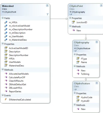
5.1. Model classes
In order to implement the presented model in the form of a functional library, a certain number of classes describing model configuration, individual sub-catchments and, finally, each hydrologic response unit, were developed. In order to define the calculation procedures, firstly present the most important classes, as well as their mutual links, will be presented.
5.2. Class for configuration of complex basins
The central class of the document is the one that contains the configurations of complex basins formed for simulation purposes. The task of the presented class of the hydrologic document is to extract all required data on simulated basins, their linking based on the hydrologic network of flows and runoff propagation in complex situations, when a larger number of basins shall be
simulated simultaneously. The document in the collection mWatersheds stores the objects of all
basins that are simulated.
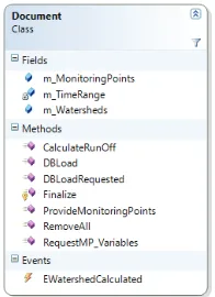
Fig. 8. Class for configuration of complex basins
The function DBLoad is used for formation of the document based on the configuration and
the parameters in the database. This function initiates the chain process of creation and reading of sub-catchment objects, then the creation and reading of objects of each HRU and, finally, all available data on input time series (rainfall, temperature etc.). After the successful document
formation, the call of the CalculateRunOff method is used to perform sequential calculation of
runoff per basins that is, per individual hydrologic response units.
In calculation of the runoff, HIS applications communicate with the model predominantly by the means of these two functions.
5.3. Class of basin model
Class of the basin model has been formed around the collection m_HRUs representing the
physical network of hydrologic response units. In addition to the functions related to database communication, it contains the CalculateRunoff function which performs the simulation of individual elements and summarizes the data at the basin level.
Figure 9 shows that the basin class has been derived from the CHydropoint class which is
the structure inherited from the implemented ArcHydro database model.
Function DBLoadHRUs is used for the process of creation and reading of objects for each
HRU. After the successful document formation, the call of CalculateRunOff method is used to
Fig. 9. Class of the mathematical model of the basin
5.4. Class of hydrologic response unit
Hydrologic response units are mainly of square shape, except on the boundaries of multiple basins where they form an irregular shape. It is assumed that all input values of the model at the unit level are homogenous, i.e. quasi-homogenous.
In addition to many variables, the class contains a certain number of functions, the most
important of which is the function Calculate that initiates the simulation procedure. The result
of the call of this function is the new state of the hydrologic unit with generation series that represent the states of surface runoffs, underground waters, snow, soil humidity and similar. Only the total runoff series represents the input data, while other series are used for visualization of dynamics of the associated phenomena that are the cause or the consequence of runoff.
5.5. Extension of HIS user interface
In order to make possible the efficient use of the model, HIS user interface has been extended by a certain number of dialog boxes for interaction with the model (Figure 10). This interaction is reflected both in definition of the configuration, and in modification of model parameters, input series, as well as the capability of review of the results.
The basic dialog box for the access to the basin model has been developed. This provided for the following data to be presented: input time series (rainfall, temperature), sub-catchment parameters, CN parameter, vegetation parameters, soil parameters and river section types.
Fig. 10. Basic dialog box for interaction with basin model
Fig. 11. Dialog box with input time series
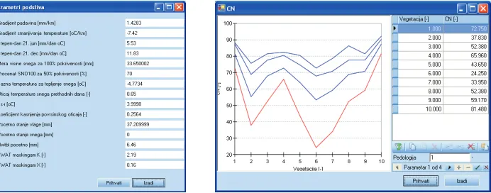
Sub-catchment parameters include the presented data typical for each sub-catchment. This data is important for the rainfall-runoff calculation based on the proposed model. Some of relevant data is presented in Figure 12.
Fig. 12. Dialog boxes with parameters of the basin model
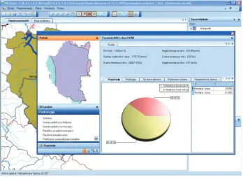
pedology, vegetation and hydrology), as well as the HRU network of the selected sub-catchment and the access to each individual HRU. Dialog boxes show their characteristics: vegetation (coverage in percentages), pedology (coverage in percentages), river section type, rainfall stations, temperature stations, total area, median elevation, length of basin flow, flow slope in the basin, length of flow down the watercourse and flow slope of the watercourse.
Fig. 13. HRU data obtained from GIS layers
6. Example of application of new model
Further below we present the example of SWAT model for the River Drina basin, with the total
area of 19232 km2. Figure 14 shows only one small sub-catchment of this catchment, from the
River Lim up to the “Prijepolje” profile (sub-catchment area covers 14.7% of the total River Drina basin).
In order to present the Drina basin faithfully, the hydrologic model has used the following data in the digital form, organized in layers: digital terrain model, river network, network of meteorological stations, pedology, vegetation, hydrogeology and the layer describing transfer of underground water to the basin and from it.
Fig. 14. Configuration of Lim River to the “Prijepolje” profile
River network. Available river network data were: rivers as lines in the vector form as 2D polygonal lines, rivers as polygons (large rivers were defined in this manner) and lakes in vector form as 2D enclosed polygons. The role of river network defined in the vector form in the hydrologic model is related to the DEM creation. For all subsequent hydrologic analyses, river network is automatically generated from DEM according to the predefined requirements regarding the upstream associated area, length, river order or similar.
Network of meteorological stations. Meteorological data (rainfall, temperature, air humidity) are given only in the form of position of meteorological stations in the basin, with their identifications and data on what is measured on the subject station (rainfall, temperature, air humidity and other).
Pedology. For the purpose of formation of the distributed hydrologic model a layer presenting the spatial distribution of soil types, i.e. pedology, is required. This layer was formed by digitalization of the pedologic atlas of 1:1000000 scale, together with classification of soil in 9 classes and mapping of these classes into 4 CN classes.
Vegetation. Vegetation in the hydrologic model has a twofold role: in the energy balance, it consumes the part of solar energy and in the hydrologic balance the water evaporates off the vegetation, i.e. it is consumed for plant growth and development. The importance of vegetation in the model is great, because the major part of water exchange takes place there. The model has a vegetation layer based on the reclassification of satellite images according to the EU recommendations set in the CORINA program.
Hydrogeology. Hydrogeologic layer is obtained by digitalization of paper layers in the 1:300000 scale, whereby the attention was paid to the separation of layers by age, water permeability and thickness. Then, all layers were classified in 9 categories.
what makes a data fund of 716,132 daily values related to these phenomena. Some 41.36% of this data is related to water levels and 59.64% to discharges. Data sources were the annual reports of the Federal and Republic Hydro-Meteorological Services. The database holds daily value of the following meteorological phenomena: daily rainfall sums on 96 rainfall or meteorological stations, daily air temperatures on 31 meteorological stations, daily values of vapor pressure on 24 meteorological stations, daily values of air humidity on 26 meteorological stations, daily sums of evaporation off the water table and vessels on 2 meteorological stations and daily snow pack height on 27 meteorological stations.
6.1. Example of simulation of runoff from basin upstream from “Prijepolje” hydrologic station
The hydrologic station “Prijepolje” covers the catchment with the total area of 2827.2 km2,
which is 14.7% of the total River Drina basin. Period chosen for simulation was from October 1st, 1982 to October 1st, 1984.
The rainfall in the subject part of the basin is observed by 8 rainfall stations, as shown in Figure 15. The average annual rainfall was 755 mm.
Air temperatures in the subject part of the basin are observed on 4 meteorological stations,
as shown in Figure 16. The average annual temperature was 7.8oC.
Fig. 15. Rainfall on the stations of the Lim River basin up to the “Prijepolje” profile during the subject period
Fig. 16. Temperatures on the stations of the River Lim basin up to the “Prijepolje” profile during the subject period
Fig. 17. Comparison of observed and simulated hydrographs on the “Prijepolje” profile
7. Conclusions
Serbia are also explained. The adapted (new) model has a detailed theoretical background and its software implementation has been performed. This paper also makes a review of the role of the SWAT model in the HIS application library (model classes and extension of the user interface) and presents an example of the model use in the River Drina basin.
This example shows that the model reacts properly during the dry and rain seasons and that it can be used successfully for annual and multiannual of simulations rainfall-runoff transformation. The example also indicates that the quality of simulation results during rain seasons is directly related to input data (rainfall, temperature and other). This is the reason why in the region of Serbia it is necessary to invest more efforts into the creation of an information environment with input data as precise possible, collected from the required number of measurement stations in the analyzed catchment.
The developed SWAT model is applicable in hydro-information systems in Serbia, as well as in the catchments and hydro-information systems in other surrounding regions (B&H, Montenegro and others). This model has been already applied in the “Drina” HIS, “Vlasina” HIS and “Vrbas” HIS. In addition to further model application, further efforts should be invested in its development and improvement. SWAT model development should be focused on the use of hourly discretization data and its application in specific hydrologic situations (such as the occurrence of flood waves and improvement of the base runoff component).
References
Arnold JG and Williams JR (1987), Validation of SWRRB: Simulator for water resources in rural basins. J. Water ResourPlan. Manage. ASCE 113(2): 243 - 256.
Arnold JG and Fohrer N (2005), SWAT2000: Current capabilities and research opportunities in applied watershed modeling. Hydrol. Process. 19(3): 563 - 572.
Arnold JG, Williams JR, Maidment DR (1995), Continuous - time water and sediment - routing model for large basins. J. Hydrol. Eng. ASCE 121(2): 171 - 183.
Bicknell BR, Imhoff JC, Donigian AS, Johanson RC (1997), Hydrological simulation program - FORTRAN (HSPF): User's manual for release 11. EPA - 600/R - 97/080. Athens, Ga.: U.S. Environmental Protection Agency
Borah DK and Bera M (2003), Watershed - scale hydrologic and nonpoint - source pollution models: Review of mathematical bases. Trans. ASAE 46(6): 1553 - 1566.
Borah DK and Bera M (2004), Watershed - scale hydrologic and nonpoint - source pollution models: Review of applications. Trans. ASAE 47(3): 789 - 803.
Cornell (2003), SMDR: The soil moisture distribution and routing model. Documentation version 2.0. Ithaca, N.Y.: Cornell University Department of Biological and Environmental Engineering, Soil and Water Laboratory. Available at: soilandwater.bee.cornell.edu/Research/smdr/downloads/SMDRmanual-v200301.pdf.
Accessed 11 February 2007.
Divac D, Grujović N, Milivojević N, Stojanović Z, Simić Z (2009), Hydro-Information Systems
and Management of Hydropower Resources in Serbia, Journal of the Serbian Society for
Computational Mechanics, Vol. 3, No. 1
El - Nasr A, Arnold JG, Feyen J, Berlamont J (2005), Modelling the hydrology of a catchment using a distributed and a semi - distributed model. Hydrol. Process. 19(3): 573 - 587. Fontaine TA, Cruickshank TS, Arnold JG, Hotchkiss RH (2002), Development of a
snowfall-snowmelt routine for mountainous terrain for the Soil and Water Assessment Tool (SWAT). J. Hydrol. 262(1-4): 209-223.
Hargreaves GL, Hargreaves GH, Riley JP (1985), Agricultural benefits for senegal River basin. J.Irrig. and Drain. Engr. 111(2):113-124.
Hargreaves GL, Hargreaves GH, Riley JP (1985), Agricultural benefits for Senegal River basin. J. Irrig. Drain. Eng. 108(3): 225-230.
Hatterman F, Krysanova V, Wechsung F, Wattenbach M (2004), Integrating groundwater dynamics in regional hydrological modelling. Environ. Model. Soft. 19(11): 1039-1051.
Institut Jaroslav Černi (2005), Hidro-informacioni sistem Drina, simulacioni model verzija 2.1,
Belgrade. Serbia.
Institut Jaroslav Černi (2007), Hidro-informacioni sistem Vlasina, simulacioni model -verzija 1,
Belgrade. Serbia.
Lenhart T, Eckhardt K, Fohrer N, Frede HG (2002), Comparison of two different approaches of sensitivity analysis. Phys. Chem. Earth 27(9-10): 645-654.
Krysanova V, Muller-Wohlfeil D-I, Becker A (1998), Development and test of a spatially distributed hydrological/water quality model for mesoscale watersheds.Ecol. Model. 106(2 - 3): 261 - 289.
Krysanova V and Badeck F (2005), A simplified approach to implement forest eco - hydrological properties in regional hydrological modelling. Ecol. Model. 187(1): 49 - 50.
Milivojević V, Divac D, Grujović N, Dubajić Z, Simić Z (2009), Open Software Architecture for
Distributed Hydro-Meteorological and Hydropower Data Acquisition, Simulation and Design
Support. Journal of the Serbian Society for Computational Mechanics, Vol. 3, No. 1
Moriasi DN, Arnold JG, Van Liew MW, Bingner RL, Harmel RD and Veith TL (2007), Model evaluation guidelines for systematic quantification of accuracy in watershed simulations. American Society for Agricultural and Biological Engineering.
Neitsch SL, Arnold JG, Kiniry JR and Williams JR (2005), The soil and water assessment tool, version 2005. http://www.brc.tamus.edu/swat/doc.html.
Olivera F, Valenzuela M, Srinivasan R, Choi J, Cho H, Koka S, Agrawal A (2006), ArcGIS - SWAT: A geodata model and GIS interface for SWAT. J. American Water Resour. Assoc. 42(2): 295 - 309.
Priestly CHB and Taylor RJ (1972), On the assessment of surface heat flux and evaporation using large - scale parameters. Monthly Weather Rev. 100(2): 81 - 92.
Prodanović D, Stanić M, Milivojević V, Simić Z, Arsić M (2009), DEM-Based GIS Algorithms
for Automatic Creation of Hydrological Models Data. Journal of the Serbian Society for
Computational Mechanics, Vol. 3, No. 1
Refsgaard JC Storm B (1995), MIKE - SHE. In Computer Models in Watershed Hydrology, 809 - 846. V. J. Singh, ed. Highland Ranch, Colo.: Water Resources Publications.
Srinivasan MS, Gerald‐Marchant P, Veith TL, Gburek WJ, Steenhuis TS (2005),
Watershed‐scale modeling of critical source areas of runoff generation and phosphorus
transport. J. American Water Resour. Assoc. 41(2): 361‐375.
Srivastava P, McNair JN, Johnson TE (2006), Comparison of process-based and artificial neural network approaches for streamflow modeling in an agricultural watershed. J. American Water Resour. Assoc. 42(2): 545-563.
Stanić M, Prodanović D, Branisavljević N (2005), Improvement of distributed hydrological
model of River Drina . Ministry of Agriculture, Forestry and Water Management.
USDA-NRCS (2004), Part 630: Hydrology. Chapter 10: Estimation of direct runoff from storm rainfall: Hydraulics and hydrology: Technical references. In NRCS National Engineering Handbook. Washington, D.C.: USDA National Resources Conservation Service. Available at: www.wcc.nrcs.usda.gov/hydro/ hydro-techref-neh-630.html. Accessed 14 February 2007.
Van Griensven A and Bauwens W (2005), Application and evaluation of ESWAT on the Dender basin and Wister Lake basin. Hydrol. Process. 19(3): 827-838.
Van Liew MW and Garbrecht J (2003), Hydrologic simulation of the Little Washita River experimental watershed using SWAT. J. American Water Resour. Assoc. 39(2): 413 - 426. Wattenbach M, Hatterman F, Weng R, Wechsung F, Krysanova V, Badeck F (2005), A