THEORY OFCOMPUTING, Volume 4 (2008), pp. 169–190
http://theoryofcomputing.org
A Quantum Algorithm for the
Hamiltonian NAND Tree
Edward Farhi
Jeffrey Goldstone
Sam Gutmann
Received: June 6, 2008; published: December 23, 2008.
Abstract: We give a quantum algorithm for the binary NAND tree problem in the Hamil-tonian oracle model. The algorithm uses a continuous time quantum walk with a running time proportional to √N. We also show a lower bound of Ω(√N) for the NAND tree problem in the Hamiltonian oracle model.
ACM Classification:F.1.2, F.2.2
AMS Classification:68Q10, 68Q17
Key words and phrases:quantum computing, NAND trees, and-or trees, game trees, quantum walk
1
Introduction
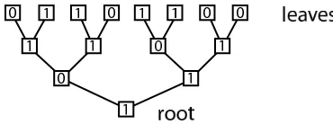
The NAND trees in this paper are complete binary trees of depthn, withN=2n leaves. Each leaf is
assigned a value of 0 or 1 and the value of any other node is the NAND of the two connected nodes just above. The goal is to evaluate the value at the root of the tree. An example is shown inFigure 1. Classically, there is a best possible randomized algorithm that succeeds after evaluating only (with high probability)O(N.753)of the leaves [10,11,12].
As far as we know, no quantum algorithm has been devised which improves on the classical query complexity. However there is a quantum lower bound ofΩ(√N) calls to a quantum oracle [2]. In this paper we are not working in the usual quantum query model but rather with a Hamiltonian oracle [6,8] which encodes the NAND tree instance. We will present a quantum algorithm which evaluates the NAND tree in a running time proportional to√N. We also prove a lower bound ofΩ(√N)on the running time for any quantum algorithm in the Hamiltonian oracle model.
Figure 1: A classical NAND tree.
Our quantum algorithm uses a continuous time quantum walk on a graph [7]. We start with a perfectly bifurcating tree of depthnand one additional node for each of theN leaves. To specify the input we connect some of theseN pairs of nodes. A connection corresponds to an input value of 1 on a leaf in the classical NAND tree and the absence of a connection corresponds to a 0. See the top of Figure 2. Next we attach a long line of nodes to the root of the tree. We call this long line the “runway.” See the bottom ofFigure 2. The Hamiltonian for the continuous time quantum walk we use here is minus the adjacency matrix of the graph. As usual with continuous time quantum walks, nodes in the graph correspond to computational basis states.
Figure 2: The full HamiltonianHO+HD.
We can decompose this Hamiltonian into an oracle,HO, which is instance dependent and a driver,
HD, which is instance independent.HDis minus the adjacency matrix of the perfectly bifurcating tree of
depthnwhose root is attached to node 0 of the line of nodes running from−MtoM. We will takeMto be very large. SeeFigure 3.
HOis minus the adjacency matrix of a graph consisting of the leaves of the bifurcating tree and the
parallel set ofNother nodes. Each leaf in the tree is connected or not to its corresponding node in the set above. SeeFigure 4. The quantum problem is: Given the Hamiltonian oracleHO, evaluate the NAND tree with the corresponding input.
Figure 4: The Hamiltonian oracleHO.
Our quantum algorithm evolves with the full HamiltonianHO+HD, which is minus the adjacency matrix of the full graph illustrated inFigure 2. The initial state is a carefully chosen right-moving packet of lengthLlocalized totally on the left side of the runway with the right edge of the packet at node 0. It will turn out thatLis of order√N. We take M to be much larger thanL, say of order L2. We now let the quantum system evolve and wait a timeL/2 which is the time it would take this packet to move a distanceLto the right if the tree were not present. We then measure the projector onto the subspace corresponding to the right side of the runway. If the quantum state is found on the right we evaluate the NAND tree to be 1 and if the quantum state is not on the right we evaluate the NAND tree to be 0.
We have chosen our right-moving packet to be very narrowly peaked in energy aroundE=0. (Note thatE=0 is not the ground state but is the middle of the spectrum.) The narrowness of the packet in energy forces the packet to be long. If we did not attach the bifurcating tree at node 0, the packet would just move to the right and we would find it on the right when we measure. The algorithm works because with the tree attached the transmission coefficient atE =0 is 0 if the NAND tree evaluates to 0 and the transmission coefficient atE=0 is 1 if the NAND tree evaluates to 1. The transmission coefficient is a rapidly changing function ofE but for|E|<1/(γ
√
N), whereγ isN-independent and large, the transmission coefficient is not far from its value atE=0. To guarantee that the packet consists mostly of energy eigenstates with their energies in this range, we takeLto beγ
√
N. This determines theO(√N)
run time of the algorithm.
Our algorithm uses the driver HamiltonianHD to evaluate the NAND tree. An arbitrary algorithm can add any instance independentHA(t)toHOand work in the associated Hilbert space. We will show that for any choice of instance independentHA(t)the running time required to evaluate the NAND tree
associated withHOis of order at least√N.
2
Motion on the runway
Here we describe the evolution of a quantum state initially localized on the left side of the runway in Figure 2headed to the right. M is so large that we can take it to be infinite as is justified by the fact that the speed of propagation is bounded. First consider the infinite runway with integersrlabeling the sites. The tree is attached atr=0. We then have for allrnot equal to 0:
Forθ >0,eirθ ande−irθ correspond to the same energy (nonnormalized) eigenstate of equation (2.1) with energy
E(θ) =−2 cosθ
but the first is a right-moving wave and the second is a left-moving wave. We are interested in a packet, that is, a spatially finite superposition of energy eigenstates, which is incident from the left on the node 0 and the attached tree. This packet will reflect back and also transmit to the right side of the runway. The packet is dominated by energy eigenstates,|Ei, of the form on the runway
hr|Ei=
(
eirθ+R(E)e−irθ
forr≤0,
T(E)eirθ forr≥0. (2.2)
(The states|Eido not vanish in the tree.) There are other energy eigenstates, but we will not need them after the discussion in the next paragraph.
Our ultimate aim is to calculate matrix elementshr|e−iHt|si, whererandslabel sites on the runway. To this end we need a completeness relation involving all of the energy eigenstates. Standard scattering theory strongly suggest that this will be
1=
π
Z
0
dθ
2π |E(θ)ihE(θ)|+contributions of other eigenstates, (2.3)
i. e., that the way the scattering states are normalized is not changed by the presence of the finite tree scatterer. We now demonstrate this.1 For the sake of brevity we make use of the special properties of our Hamiltonian, though the result is much more general. For the rest of this paragraph only, we relabel the states defined in (2.2) as|E,→i. There are also states, which can be superposed to make left-moving packets, incident on the tree from the right. NowH commutes with the reflection operator,Π, defined
by
Π|ri=| −ri whererlabels a site on the runway
Π|ii=|ii whereilabels a site on the tree. (2.4)
We can obtain the left-moving energy eigenstate|E,←iby
|E,←i=Π|E,→i, (2.5)
so that on the runway
hr|E,←i=
(
T(E)e−irθ forr60,
e−irθ+R(E)eirθ
forr>0. (2.6)
The states|E,±i=|E,←i ± |E,→iare simultaneous eigenstates ofH andΠ. There might also be a
finite set of orthonormal energy eigenstates{|Eki}, either bound states withhr|Eki →0 exponentially as |r| →∞, or states entirely confined to the tree, i. e., withhr|Eki=0 on the runway. SinceHandΠare
commuting self-adjoint operators, the spectral theorem asserts that there are measures f±(θ)dθ such that
1= Z π
0
f+(θ)dθ|E(θ),+ihE(θ),+| + Z π
0
f−(θ)dθ|E(θ),−ihE(θ),−|
+
∑
k
|EkihEk|. (2.7)
We are assuming here that the measures are absolutely continuous with respect to Lebesgue measure. In terms of the left and right-moving states (2.7) becomes
1= Z π
0
f(θ)dθ
|E(θ),→ihE(θ),→ |+ |E(θ),←ihE(θ),← |
+ Z π
0
g(θ)dθ
|E(θ),→ihE(θ),← |+ |E(θ),←ihE(θ),→ |
+
∑
k
|EkihEk|.
(2.8)
We determine f(θ)andg(θ)by calculatinghr|1|si=δr,sin the two casesr→ −∞,s→ −∞, with the
difference r−s=mfixed, andr→ −∞,s→+∞,withr+s=mfixed, making use of the relations
|R(E)|2+|T(E)|2=1
R(E)T∗(E) +R∗(E)T(E) =0. (2.9)
These follow from the self-adjointness and reflection symmetry ofH, but for our specialHcan be seen from the explicit expressions forT(E)andR(E)in terms of a real functiony(E)that we have in (2.15) and (2.17). Withr<0,s<0, we find
hr|1|si= Z π
0
f(θ)dθ
ei(r−s)θ+e−i(r−s)θ+R(E)ei(r+s)θ+R∗(E)ei(r+s)θ
+ Z π
0
g(θ)dθ
T(E)e−i(r+s)θ+T∗(E)ei(r+s)θ
+
∑
k
hr|EkihEk|si.
(2.10)
Whenr,s→ −∞, the integrals linear inR(E) andT(E)go to zero by the Riemann-Lebesgue Lemma,
and the terms involving|Ekialso go to zero, so withr−s=mwe obtain
2
Z π
0
f(θ)cosmθdθ=δm,0. (2.11)
This determines f(θ) =1/2π. Withr<0, s>0, we find
hr|1|si= Z π
0
f(θ)dθ
T(E)e−i(r−s)θ+T∗(E)ei(r−s)θ
+ Z π
0
g(θ)dθ
ei(r+s)θ+e−i(r+s)θ+R(E)e−i(r−s)θ+R∗(E)ei(r−s)θ
+
∑
k
Whenr→ −∞, s→+∞withr+s=m, we obtain
2
Z π
0
g(θ)dθcosmθ=0. (2.13)
Thus determinesg(θ) =0, so that we have the desired completeness relation
1= 1
2π
Z π
0
dθ
|E,→ihE,→ |+|E,←ihE,← |
+
∑
k
|EkihEk|. (2.14)
We will use this completeness relation to prove our results. In particular we will only get relevant contributions from the first term and we go back to (2.2) with the symbol→dropped.
Returning to (2.2) and looking atr=0 we see that
1+R(E) =T(E). (2.15)
The transmission coefficientT(E)is determined by the structure of the tree. In particular let
y(E) = hroot|Ei
hr=0|Ei (2.16)
where “root” is the node immediately abover=0 on the runway, seeFigure 2. Applying the Hamiltonian at|r=0igives
H|r=0i=−|r=−1i − |r=1i − |rooti
and taking the inner product with|Eigives
T(E) = 2isinθ
2isinθ+y(E). (2.17)
In the next section we will show how to calculatey(E)and show that if the NAND tree evaluates to 1 theny(0) =0 meaning thatT(0) =1 and if the NAND tree evaluates to 0 theny(0) =∞andT(0) =0.
Unfortunately we cannot build a state with onlyE=0 since it would be infinitely long. Instead we build a finite packet that is long enough so that it is effectively a superposition of the states|EiwithE close enough to 0 thatT(E)is close toT(0). We introduce two parametersε andDfor which
|T(E)−T(0)|<D|E| for |E|<ε. (2.18)
The parametersε andDdo depend on the size of the tree, but for the remainder of this section we only useε 1.
The initial state we consider,|ψ(0)i, is given on the runway as
hr|ψ(0)i=
( 1
√
Le
irπ/2 for−L+1≤r≤0,
0 forr≤ −Landr>0 . (2.19)
and vanishes in the tree. For this state
hψ(0)|H|ψ(0)i=0
so the spread in energy about 0 is of order 1/√L. However, for our purpose we will see that this state is effectively more narrowly peaked in energy, and (2.20) is really an artifact of its sharp edge. In fact most of the probability in energy is contained in a peak around 0 of width 1/L. Because we takeπ/2 and not−π/2 in (2.19) we have a right-moving packet with energies near 0.
Evolving with the full Hamiltonian of the graph we have
|ψ(t)i=e−iHt|ψ(0)i.
We decompose|ψ(t)iinto two orthogonal parts,
|ψ(t)i=|ψ1(t)i+|ψ2(t)i
where
|ψ1(t)i= π
2+ε Z
π
2−ε dθ 2π e
−itE(θ)|E(
θ)i hE(θ)|ψ(0)i (2.21)
and|E(θ)iis given in (2.2) with the completeness relation (2.3). The state|ψ2(t)iis a superposition of the other eigenstates ofH, that is, states incident from the left with 0<θ <π2−ε and π2+ε <θ <π, states incident from the right and bound states with|E|>2 andhr|Ei →0 exponentially asr→ ±∞on
the runway. We do not need the details of|ψ2(t)isince we will show inSection 5that the norm of|ψ1(t)i is close to 1 so the norm of|ψ2(t)iis near 0. In other words, |ψ1(t)iis a very good approximation to |ψ(t)i. To ensure this we need
L 1 ε.
We would then expect that at late enough times we will see on the right a packet like the incident packet, but multiplied byT(0) and moving to the right, with the group velocitydE/dθ evaluated atθ =π/2 which is 2. InSection 5we show, iftis not too big, that forr>0
hr|ψ(t)i=T(0)hr−2t|ψ(0)i (2.22)
plus small corrections. (InSection 5 we also make sense of this equation for 2t not an integer.) To ensure (2.22) we also need
LD2ε.
Since |ψ(0)i is a normalized state localized between r=−L+1 and r=0, (2.22) implies that for
t>L/2
∑
r>0
|hr|ψ(t)i|2=|T(0)|2
3
Evaluating the transmission coefficient near
E
=
0
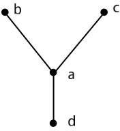
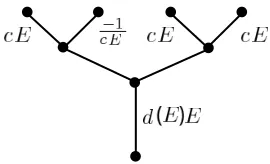
From the last section, equation (2.17), we see that we can findT(E)if we knowy(E). We now show how the structure of the tree recursively determinesy(E). Consider the tree in Figure 2 ignoring the runway but including the runway node atr=0. Except at the top or bottom of this tree every node is connected to two nodes above and one below. SeeFigure 5wherea,b,canddare the amplitudes of|Ei at the corresponding nodes.
Figure 5: The amplitudes at 4 nodes in the middle of the tree in an energy eigenstate.
ApplyingHat the middle node yields:
E a=−b−c−d
from which we get
Y =− 1
E+Y0+Y00
whereY =a/d,Y0=b/aandY00=c/a. This is shown pictorially inFigure 6. Theywe seek isY at
Figure 6: The recursion forY.
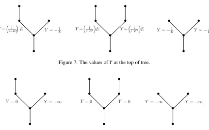
the bottom of the tree. To find it we recurse down from the top of the tree. At the top of the tree there are 3 possibilities with the respective values ofY obtained by applying the Hamiltonian. The results are shown inFigure 7. From Figures6and7we see thatY(−E) =−Y(E)so we can restrict attention to
E>0.
Figure 7: The values ofY at the top of tree.
Figure 8: The values ofY at the top of the tree asE→0+.
recursion asE→0+there are two initial values ofY which are -∞and 0. Returning toFigure 6with
the different possibilities forY0 andY00 we get Figure 9. IdentifyingY =0 with the logical value 1 andY =−∞with the logical value 0 we see thatFigure 9is a NAND gate. Accordingly the value of y(0) =Y(0)at the bottom of the tree (see (2.16) andFigure 2) is the value of the NAND tree with the input specified at the top.
Figure 9: The recursion forY atE=0 implements the NAND gate.
We now move away fromE=0 to see how far fromE=0 we can go and still have the value of the NAND tree encoded iny(E)at the bottom. NearE=0 it is convenient to writeY(E)either asa(E)Eor
as−1/(b(E)E)and we will find bounds on how largea(E)andb(E)can become as we move down the
not too big. To see this use the recursive formula inFigure 6. There are three cases and we obtain figure (10) which makes the increasingness clear.
Figure 10: The coefficient ofE inY is an increasing function ofa,a0,bandb0.
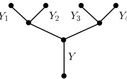
Now consider a piece of the bifurcating tree as depicted inFigure 11. There are 4 different values of
Figure 11:Y determined by four values ofY above.
Y at the top of the piece, which determineY at the bottom of the piece. Suppose for 0<E<2−n/2/16 each of theY at the top of the piece obeys
0≤Yi(E)≤c E or 0≤ −1
Yi(E) ≤c E
for some positivecwithc+1≤4·2j where j≤n/2. We will show
0≤Y(E)≤c∗E or 0≤ −1
Y(E)≤ c
∗
E (3.1)
where
(c∗+1) = 2(c+1)
1−2−n+2j/4. (3.2)
There are six cases to consider and here we exhibit the most dangerous case; seeFigure 12.
The reason we can use the coefficientcon the four top edges is the increasingness referred to earlier.
HereY(E) =d(E)E. Using the recursion fromFigure 10we get
d(E) = 2c+1
1−1+1−(1+c)cEc 2
(2c+1)E2
≤ 2c+1
Figure 12: The most dangerous case.
using(1+c)≤4·2n/2andE2≤ 1 1622
−n. So
d(E)≤ 2c+1 1−4(1+c)2E2 ≤
2(c+1)
1−4(1+c)2E2−1≤
2(c+1)
1−22j−n/4−1, (3.3)
using 1+c≤4·2j andE ≤2−n/2/16. From (3.3) we get the left side of (3.1) withc∗ given in (3.2). (FromFigure 10, the bounds oncandEalso imply that the coefficients remain positive from one level to the next, so 0≤Y(E).) The other cases yield smaller coefficients and we will not run through them here.
At the top of the full treeY(E) =E/(1−E2)orY(E) =−1/Eas can be seen fromFigure 7. Given the restrictionO<E<2−n/2/16 we can take
ctop= 1
1−2−n. (3.4)
Moving down the tree we get aftern/2 iterations of (3.2) with j=1,2, . . .n/2,
(c∗bottom+1) = ctop+1
2 1−22−n/4
2 1−24−n/4
. . .
2 1−2n−n/4
. (3.5)
Therefore
c∗bottom≤ 1+ 1 1−2−n
2n/2
1−1 4∑
n/2
j=122j−n
≤ 1+
1 1−2−n
2n/2
1−1 3
≤4·2n/2
also justifying the assumptionc≤4·2jat each step.
This means that|y(E)|at the bottom is either less than|c∗bottomE|or greater than|1/(c∗bottomE)|for |E|< 2−n/2/16. The crucial√Narose because the coefficients ofY(E)could barely more than double as we movedtwolevels down the tree.
Going back to the relation betweeny(E)and the transmission coefficient given in (2.17) we summa-rize our results for this section:
NAND = 0 (reflect) |y|> 1
4√N|E| |T|<8 √
N|E| for|E|< 1
16√N
NAND = 1 (transmit) |y|<4√N|E| |T−1|<3√N|E| for|E|< 1
4
Putting it all together
Here we combine the results of Sections2and3 and state the algorithm. First, the algorithm. Given the Hamiltonian oracle corresponding to an instance of the NAND tree problem we construct the full HamiltonianHO+HDwhich is minus the adjacency matrix of the graph inFigure 2. We then build the
initial state
|ψ(0)i=√1
L
0
∑
r=−L+1
eirπ/2|ri (4.1)
whereris on the runway. We choose
L=γ √
N (4.2)
withγ1 a constant independent ofN. We let the state evolve for a time
trun=L
2 (4.3)
and then measure the projectorP+onto the right side of the runway
P+= M
∑
r=1
|rihr|. (4.4)
If the measurement yields 1 we evaluate the NAND tree to be 1 and if the measurement yields 0 we evaluate the NAND tree to be 0.
According to the results stated inSection 2, the probability of getting a measurement result of 1 is very near|T(0)|2if
L 1
ε and LD
2
ε. (4.5)
From the table at the end ofSection 3we can take
ε= 1
16√N (4.6)
and
D=8 √
N (4.7)
and then the choiceγ1 ensures (4.5). At the end of section5we will see that the error probability of the algorithm isO√1
Lε,D q
ε
L,
ε
L
1/4
which isOq1
γ
for largeN. By choosingγlarge enough we can make the success probability as close to 1 as desired.
5
Technical details
Here we flesh out the claims made inSection 2and put bounds on the corrections to the stated results. Since we work withθclose toπ/2 it is convenient to write
and
E(ϕ+π/2) =2 sinϕ
so (2.21) becomes
|ψ1(t)i=
ε
Z
−ε
dϕ 2π e
−2itsinϕ|E(
ϕ+π/2)ihE(ϕ+π/2)|ψ(0)i
whereεis the small parameter introduced in (2.18). Using (2.2) gives
hE(ϕ+π/2)|ψ(0)i= √1
L L−1
∑
r=0
eirϕ+ (−1)r
R∗(E)e−irϕ .
We now break|ψ1(t)iinto two pieces
|ψ1(t)i=|ψA(t)i+|ψB(t)i
where
|ψA(t)i=
ε
Z
−ε
dϕ 2π e
−2itsinϕA(
ϕ)|E(ϕ+π/2)i (5.1)
with
A(ϕ) =√1
L L−1
∑
r=0
eirϕ =√1
L
eiLϕ−1
eiϕ−1 (5.2)
and
|ψB(t)i=
ε
Z
−ε
dϕ 2π e
−2itsinϕ R∗(E)B(
ϕ)|E(ϕ+π/2)i
with
B(ϕ) =√1
L L−1
∑
r=0
(−1)re−irϕ =√1
L
1−(−1)Le−iLϕ
1+e−iϕ .
Note that|ψA(t)iand|ψB(t)iare not orthogonal. Now
|B(ϕ)|2< 1
Lcos2 1 2ε
for |ϕ|<ε
and|R(E)| ≤1 so
hψB(t)|ψB(t)i=
ε
Z
−ε
dϕ 2π |R(E)|
2|B( ϕ)|2
is of orderε/Land we have
|ψB(t)i
On the other hand
hψA(t)|ψA(t)i=
ε
Z
−ε
dϕ
2π |A(ϕ)|
2. (5.4)
Now
π
Z
−π
dϕ
2π |A(ϕ)| 2= 1
L L−1
∑
r=0
1=1 (5.5)
while
−ε
Z
−π
dϕ 2π |A(ϕ)|
2+
π
Z
ε
dϕ
2π |A(ϕ)| 2= 1
π
π
Z
ε
dϕ1
L
sin12Lϕ
sin12ϕ
!2
< π
Lε (5.6)
since sinϕ2 >ϕ
π and(sin
1
2Lϕ)2<1. Combining (5.4), (5.5) and (5.6) gives
1− π
Lε <
hψA(t)|ψA(t)i ≤1
so |ψA(t)i
=1−O
1
Lε
. (5.7)
We now require
L 1 ε so the norm of|ψA(t)iis close to 1.
Now
|ψ1(t)i
≥ |ψA(t)i
− |ψB(t)i
so |ψ1(t)i
=1−O
1
Lε,
r
ε
L
whereO(a,b) meansOof the larger ofaandb. This justifies our claim inSection 2 that|ψ1(t)iis a very good approximation to the true evolving state|ψ(t)i. Since
|ψ1(t)i
2 + |ψ2(t)i
2 =1
we also have
|ψ2(t)i
=O 1 √ Lε ,ε L
1/4
. (5.8)
We measure the state|ψ(t)ion the right side of the runway, so we need a good estimate of
hψ(t)|P+|ψ(t)i=
∑
r>0
hr|ψ(t)i 2 . Using
and the bounds on the norms (5.3), (5.7) and (5.8) we get
hψ(t)|P+|ψ(t)i=hψA(t))|P+|ψA(t)i+O
1 √ Lε ,ε L
1/4
(5.9)
so we can use|ψA(t)ito estimate the probability of finding the state on the right at timet. Now forr≥0 from (2.2) and (5.1)
hr|ψA(t)i=
ε
Z
−ε
dϕ 2π e
−2itsinϕT(E)A(
ϕ)ireirϕ.
Let
ar(t) =T(0)ir
π
Z
−π
dϕ 2π e
i(r−2t)ϕA(
ϕ). (5.10)
We want to show thatar(t)is a good approximation tohr|ψA(t)i. We can write
hr|ψA(t)i=ar(t) +br(t) +cr(t) +dr(t) (5.11)
with
br(t) = −irT(0)
−ε Z −π dϕ 2π +
π Z ε dϕ 2π
ei(r−2t)ϕA(
ϕ),
cr(t) = irT(0)
ε
Z
−ε
dϕ 2π(e
−2itsinϕ −e−2itϕ)eirϕA(
ϕ)
and
dr(t) = ir
ε
Z
−ε
dϕ
2π (T(E)−T(0))e
−2itsinϕeirϕA(
ϕ).
We now show thatbr(t),cr(t)anddr(t)are small. First
∞
∑
r=0
|br(t)|2<
∞
∑
−∞|br(t)|2=|T(0)|2·2·
π
Z
ε
dϕ 2π |A(ϕ)|
2
by Parseval’s Theorem. Using (5.6) we have
∞
∑
r=0
|br(t)|2=O
1
Lε
Similarly
∞
∑
r=0
|cr(t)|2<|T(0)|2
ε Z −ε dϕ 2π e
2it(ϕ−sinϕ)−1
2 |A(ϕ)|2
=|T(0)|2
ε Z −ε dϕ 2π 1 9t 2
ϕ6+· · ·
1
L
sin2 12Lϕ
sin2 12ϕ .
(5.13)
However we taketrunto be nearL/2. As long asLε31 we have
∞
∑
r=0
|cr(t)|2=O(Lε5). (5.14)
To keep this small we needLε51, but this follows from our assumption thatLε31 sinceε 1. The assumption thatLε31 helps us to establish the translation property in (2.22) which simplifies the picture of what is going on. Also
∞
∑
r=0
|dr(t)|2<
ε
Z
−ε
dϕ 2π
|T(E)−T(0)|2|A( ϕ)|2.
Using|T(E)−T(0)|<D|E| for |E|<εwe get
∞
∑
r=0
|dr(t)|2 < D2
ε
Z
−ε
dϕ 2π 4 sin
2 ϕ 1
L
sin2(12Lϕ)
sin2(12ϕ) (5.15)
= O
D2ε
L
(5.16)
from which we get our condition
LD2ε.
Now from (2.19) and (5.2) we have
hr|ψ(0)i=ir
π
Z
−π
A(ϕ)eirϕdϕ. (5.17)
So from (5.10) we see that
ar(t) =T(0)hr−2t|ψ(0)i (5.18)
but only when 2tis an integer. However if 2t=m+τ withman integer and 0≤τ <1,
∞
∑
−∞|ar(t)−ar
m
2
|2 = |T(0)|2
π Z −π dϕ 2π 1 L
sin2 12Lϕ
sin2 12ϕ
|eiτ ϕ−1|2
We have shown that forr>0,hr|ψ(t)iis well approximated byhr|ψ1(t)iwhich is well approximated byhr|ψA(t)iwhich is well approximated byar(t)which has the form (5.18) so (2.22) is justified.
Furthermore, using (5.9), (5.11), (5.12), (5.14), (5.16) and (5.18) we have fort>L/2
hψ(t)|P+|ψ(t)i=|T(0)|2 + O
1 √
Lε
,D
r
ε
L,
ε
L
1/4
(5.20)
which can be used to estimate the failure probability of the algorithm.
6
A lower bound for the Hamiltonian NAND tree problem via the
Hamil-tonian Parity problem
Here we show that if the input to a NAND tree problem is given by the Hamiltonian oracleHOdescribed inSection 1then for an arbitrary driver HamiltonianHA(t), evolution usingHO+HA(t)cannot evaluate the NAND tree in a time of order less than√N. This means that our algorithm which takes time√N is optimal up to a constant.
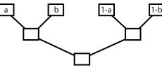
In the usual query model, the parity problem with√N variables can be embedded in a NAND tree withN leaves [2]. To see this first consider 2 variables,a andb, and the 4 leaf NAND tree given in Figure 13which evaluates to(1+a+b)mod 2. Using this we see that with 4 variablesa,b,c,d the NAND tree inFigure 14evaluates to(1+a+b+c+d)mod 2. This clearly continues. Since we know that the parity problem for√Nvariables cannot be solved with less than of order√Nquantum queries, we know that the NAND tree problem cannot be solved with fewer than of order√Nquantum queries.
Figure 13: This NAND tree evaluates to(1+a+b)mod 2.
Figure 14: This NAND tree evaluates to(1+a+b+c+d)mod 2.
not included (just as inFigure 4) and accordingly the corresponding Hamiltonian matrix element is 0.A
label−1 means that the edge is there (just as inFigure 4) and the corresponding matrix element of the Hamiltonian oracle is−1.
Figure 15: The Hamiltonian oracle for the NAND tree set up to evaluate(1+a+b+c+d)mod 2. The coefficients are 0 or−1 corresponding to the edge present or not.
We see that the Hamiltonian parity problem can be embedded in the Hamiltonian NAND tree prob-lem. We did this for the Hamiltonian NAND tree oracle considered in this paper, but it can also be done for the more general Hamiltonian NAND tree oracle described in the Conclusion.
We will now prove a lower bound for the Hamiltonian parity problem, in a general setting (see also [8]), which can be used to obtain a√N lower bound for the Hamiltonian NAND tree problem. The oracle for the parity problem is a Hamiltonian of this form:
HOP= K
∑
j=1
Hj. (6.1)
TheHj operate on orthogonal subspacesVj with
Hj=PjHjPj
wherePj is the projection ontoVj. Furthermore we assumekHjk ≤1. For each jthere are two possible
operatorsH(aj j),aj=0 or 1. The stringa1,a2, . . . ,aKis the input to the parity problem to be solved. In
the Hamiltonian oracle model, an algorithm can use (6.1), but has no other access to the stringa. This is the most general form for the parity oracle Hamiltonian that we can imagine and it certainly includes the oracle we used to embed Hamiltonian parity in the Hamiltonian NAND tree.
Choose an arbitrary driver HamiltonianHA(t). Let S be an instance of parity, that is, a subset of
1,2, . . . ,K with aj=1 iff j is an element of S. Starting in an instance independent state |ψ(0)i we
evolve for timeT according to the Schr¨odinger equation
i d
dt|ψS(t)i=HS(t)|ψS(t)i
using the total HamiltonianHS(t)
HS(t) =g(t)HOP+HA(t)
where|g(t)| ≤1. With the inclusion of the coefficientg(t)it is clear that the Hamiltonian oracle model includes the quantum query model.
Let|ψS(T)ibe the state reached at timeT. A successful algorithm for parity must have
for someKindependentδ >0 if the parity ofSandS0differ. We now show that this suffices to forceT to be of orderK. Our approach is an analogue to the analog analogue [6] of the BBBV method [3]. We writeS∼S0ifSandS0 differ by one element. Summing on(S,S0)which differ by one element gives
d dtS
∑
∼S0
|ψS(t)i − |ψS0(t)i
2
=
∑
S∼S0
2 ImhψS(t)|(HS(t)−HS0(t))|ψS0(t)i
=
∑
S∼S0
2 ImhψS(t)| ± 4j(S,S0)|ψS0(t)i
where j(S,S0)is the element by whichSandS0differ, and4j=g(t)
H(j1)−H(j0). The+sign means that j(S,S0)∈Swhereas the−sign means that j(S,S0)∈S0. Now we have
d dtS
∑
∼S0
|ψS(t)i − |ψS0(t)i
2
≤2
∑
S∼S0
hψS(t)|Pj(S,S0)4j(S,S0)Pj(S,S0)|ψS0(t)i
≤4
∑
S∼S0
Pj(S,S0)|ψS(t)i ·
Pj(S,S0)|ψS0(t)i
sincek4jk ≤2. Usingab≤ 12a2+12b2
gives
d dtS
∑
∼S0
|ψS(t)i − |ψS0(t)i
2
≤2
∑
S∼S0
Pj(S,S0)|ψS(t)i 2 +
Pj(S,S0)|ψS0(t)i
2
.
For fixedS0, j(S,S0)runs over{1,2, . . . ,K}so
∑
S∼S0,S0fixed
Pj(S,S0)|ψS0(t)i
2 ≤1
and similarly for fixedSand thus we have
∑
S∼S0
Pj(S,S0)|ψS(t)i 2 +
Pj(S,S0)|ψS0(t)i
2
≤2·2K
since there 2K possibilities forS0 (orS). We’ve shown that
d dt S
∑
∼S0
|ψS(t)i − |ψS0(t)i
2
≤4·2K,
and since
∑
S∼S0
|ψS(0)i − |ψS0(0)i
2
=0
we can integrate to obtain
∑
S∼S0
|ψS(T)i − |ψS0(T)i
2
For eachS0 there areKchoices ofS, so a successful algorithm requires
∑
S∼S0
|ψS(T)i − |ψS0(T)i
2
≥2K·K·δ
and we have the desired bound
T ≥Kδ/4.
Conclusion
We are not working in the quantum query model but rather in the quantum Hamiltonian oracle model. In this model the programmer is given a Hamiltonian oracle of the form
HO= N
∑
j=1
Hj
where theHj operate in orthogonal subspaces. Each Hj is one of two possible operators H (bj) j with bj =0 or 1 and the stringb1· · ·bN is the input to the classical NAND tree that is to be evaluated. The quantum programmer is allowed to evolve states using any Hamiltonian of the formg(t)HO+HA(t)
where the coefficientg(t)satisfies|g(t)| ≤1 andHA(t)is any instance independent Hamiltonian. The
programmer has no other access to the stringb.
The algorithm presented in this paper uses a time independentHO+HDwhich is (minus) the
adja-cency matrix of a graph, so our algorithm is a continuous time quantum walk. We evaluate the NAND tree in time of order√Nwhich is (up to a constant) the lower bound for this problem.
After the arXiv version of this paper appeared, corresponding results in the discrete-query model were obtained [1,4]. Further generalizations to other formulas can be found in [5,9].
Acknowledgement
Two of the authors gratefully acknowledge support from the National Security Agency (NSA) and the Disruptive Technology Office (DTO) under Army Research Office (ARO) contract W911NF-04-1-0216. We also thank Richard Cleve for repeatedly encouraging us to connect continuous time quantum walks with NAND trees, and for discussions about the Hamiltonian oracle model. We thank Andrew Landahl for earlier discussions of the NAND tree problem.
References
[1] * ANDRIS AMBAINIS, ANDREW M. CHILDS, BEN W. REICHARDT, ROBERT ˇSPALEK, AND
[2] * HOWARD BARNUM AND MICHAEL SAKS: A lower bound on the quantum query complexity of read-once functions. J. Comput. System Sci., 69(2):244–258, 2004. [doi:10.1016/j.jcss.2004.02.002].1,6
[3] *CHARLESH. BENNETT, ETHANBERNSTEIN, GILLESBRASSARD, ANDUMESHVAZIRANI:
Strengths and weaknesses of quantum computing. SIAM J. Comput., 26(5):1510–1523, 1997. [doi:10.1137/S0097539796300933].6
[4] * ANDREW M. CHILDS, RICHARD CLEVE, STEPHEN P. JORDAN, AND DAVID YEUNG: Discrete-query quantum algorithm for NAND trees, 2007. [arXiv:quant-ph/0702160].6
[5] *RICHARDCLEVE, DMITRYGAVINSKY,ANDDAVIDL. YEUNG: Quantum algorithms for eval-uating MIN-MAX trees, 2007. [arXiv:0710.5794].6
[6] *EDWARDFARHI ANDSAMGUTMANN: An analog analogue of a digital quantum computation.
Phys. Rev. A, 57:2403, 1998. [doi:10.1103/PhysRevA.57.2403]. 1,6
[7] * EDWARD FARHI AND SAM GUTMANN: Quantum computation and decision trees. Phys. Rev. A, 58:915, 1998. [doi:10.1103/PhysRevA.58.915].1
[8] * CARLOS MOCHON: Hamiltonian oracles. Phys. Rev. A, 75:042313, 2007.
[doi:10.1103/PhysRevA.75.042313].1,6
[9] *BENW. REICHARDT ANDROBERT ˇSPALEK: Span-program-based quantum algorithm for
eval-uating formulas. InProc. 40th STOC, pp. 103–112. ACM, 2008. [doi:10.1145/1374376.1374394]. 6
[10] * MICHAEL SAKS AND AVI WIGDERSON: Probabilistic boolean trees and the complexity of evaluating game trees. InProc. 27th FOCS, pp. 29–38. IEEE Computer Society, 1986. 1
[11] *MIKLOSSANTHA: On the Monte Carlo Boolean decision tree complexity of read-once formulae.
Random Structures Algorithms, 6(1):75–87, 1995. [doi:10.1002/rsa.3240060108].1
[12] * MARCSNIR: Lower bounds on probabilistic decision trees. Theoret. Comput. Sci., 38:69–82, 1985. [doi:10.1016/0304-3975(85)90210-5].1
AUTHORS
Edward Farhi[About the author]
Cecil and Ida Green Professor of Physics Massachusetts Institute of Technology Cambridge, MA 02139
farhi mit edu
Jeffrey Goldstone[About the author]
Cecil and Ida Green Professor of Physics, Emeritus Massachusetts Institute of Technology
Cambridge, MA 02139 goldston mit edu
http://web.mit.edu/physics/facultyandstaff/faculty/jeffrey goldstone.html
Sam Gutmann[About the author]
Department of Mathematics
Northeastern University, Boston MA sgutm neu edu
http://www.math.neu.edu/∼Gutmann/
ABOUT THE AUTHORS
EDWARD FARHI is a professor of physics and the director of the Center for Theoretical PhysicsatMIT. He is a lapsed particle physicist hoping to return to his roots when data from experiments offers new insight into how the world really works. Meanwhile he works on quantum computation, primarily focusing on algorithm design. He started collaborating with Sam in high school and with Jeffrey at MIT.
JEFFREY GOLDSTONE, after 25 years at Cambridge University and 30 at MIT, is now Professor of Physics Emeritus. He worked on many-body theory and in the prehistoric eras of the standard model and string theory. He has been helping Eddie and Sam search for quantum algorithms for the last 10 years.
SAM GUTMANN crosses the river (from the math department atNortheastern University)