Vol. 2 Issue 12, December - 2016
Numerical Modeling of Flow Pattern in
rectangular shallow Basins
Hamed Sarveram
Assistant Professor, Department of Civil engineering,
Zanjan Branch, Islamic Azad University, Zanjan,Iran.
(Corresponding Author)
Mehdi Shahrokhi
Assistant Professor of Ghiaseddin Jamshid Kashani Higher Education Institute,Iran.
Farshad Shariati
M.S. Student of Ghiaseddin Jamshid Kashani Higher
Education Institute,Iran.
Abstract— in this research by using numerical modeling, Flow pattern is investigated under the various flow conditions and basin geometry, in shallow basins. The government equations are shallow water equations and semi- lagrangian method is used to solve these equations. The results show that the proposed model acceptably Simulates flow behavior in the shallow rectangular basin. In addition, research on the effect of basin dimensional on flow pattern show that for the basin which aspect ratio (length to width) greater than 1.2, non-Symmetrical flow is established approximately. Otherwise, Flow pattern is symmetric in the rectangular basin.
Keywords— rectangular shallow Basins; flow pattern; Numerical modelling; semi- lagrangian method.
I. INTRODUCTION
Inflow velocity is reduced by increasing the flow cross section; and accordingly of sediment particles will deposit. Therefore, during designing the basin or reservoirs their tasks should be concentrate, e.g., in settling basin, sedimentation must to be maximum. But, in Dam reservoirs this volume must to be minimum.
One of the important issues of sedimentation process in basins is Flow pattern. Consequently, flow pattern in rectangular basin, under the various flow conditions and basin geometry is investigated.
Reference [1] studied flow patterns in several shallow rectangular basins. Their results show that the flow pattern might become asymmetric even if the inflow and outflow conditions were symmetric. Reference [2] studied flow patterns in rectangular basins by the lattice Boltzmann model. The results showed that their model could predict flow pattern with comparable accuracy with conventional method using an algebraic model for flow turbulence. Also, the results indicate by increasing Froude number and bed roughness, the flow patterns have less deviation from symmetric and the reattachment length increase. Reference [3] simulated symmetric and asymmetric flows in shallow rectangular basins with different lateral
expansion ratios lengths. Comparison between simulated results and experimental data showed a good agreement of the critical shape parameter between symmetric and asymmetric flows.
II. GOVERNING EQUATIONS
The depth-averaged, shallow water equations were applied for this study. These equations assume hydrostatic pressure distribution, a well-mixed water column, and a small depth to width ratio:
2 2 2 2 2
4
2 2
3
U U U U U n U V
U V g g U
t y x x x y H (1)
2 2 2 2 2
4
2 2
3
V V V V V n U V
V U g g V
t y x y x y H
(2)
0
HU HV
t x y
(3)
Where U is the depth-averaged x-direction velocity
component, V is the depth averaged y-direction
velocity component, η is the free surface elevation, g
is the gravitational constant, t is time, ε is the
horizontal eddy viscosity coefficient, H is the total
water depth, h is undisturbed water depth, n is
Manning’s roughness coefficient and ,as shown in the
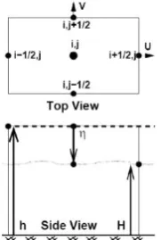
fig. 1, H = η + h.
Vol. 2 Issue 12, December - 2016
III. NUMERICAL MODELING
As shown in fig. 1, free surface elevation, η, is
defined at the center of each computational cell. Total water depth, H, and directional velocity components, U and V, are defined at the midpoint of volume faces. Undisturbed water depth, h, is also defined at the midpoint of volume faces. The finite volume structure provides a control volume representation that is inherently mass conservative [4].
The combination of an implicit free surface solution and a semi-Lagrangian representation of advection, provide advantages of a stable solution. In the implicit process, the free surface elevation in the momentum equations, equations (1 and 2), and the velocity divergence in the continuity equation, (3), is treated implicitly. The advective terms in the momentum equations are discretized explicitly. The continuity equation is discretized as follows:
1 1 1
, , 1 2, 1 2, 1 2, 1 2,
1 1
, 1 2 , 1 2 , 1 2 , 1 2
N N N N N N
i j i j i j i j i j i j
N N N N
i j i j i j i j
t
H U H U
x t
H V H V
y (4)
Where, (i, j) subscript is spatial location and the
superscript, N or N +1, represents the temporal
location, Δx and Δy represent the x and y direction
volume lengths respectively, Δt is the computational
time step duration. The numerical approximations with conservation of momentum equations, give the following equations:
1 1 1
1 2, 1 2, 1, ,
0.5
2 2
, 1 2, 1 2,
1 1 2, 4
3 1 2,
N N N N
i j i j i j i j
N N
i j i j i j
N i j N i j g t U FU x n U V
g t U
H (5)
1 1 1
, 1 2 , 1 2 , 1 ,
0.5
2 2
, , 1 2 , 1 2
1 , 1 2 4
3 , 1 2
N N N N
i j i j i j i j
N N
i j i j i j
N i j N i j g t V FV y
n U V
g t V
H (6)
Where, the FU and FV terms are the
semi-Lagrangian advection operators. A semi-semi-Lagrangian advection method employs a Lagrangian algorithm across the underlying Eulerian model grid. The Lagrangian component of the scheme traces the path line of a particle which is initially located at the volume face, that is the velocity definition location from fig. 1 going backwards along the particle path line a distance corresponding to the simulation time step duration, Δt, is obtained. The particle departure point is the location of the particle at the beginning of the current time step. Again, this location is obtained by tracing the particle backwards along the path line [5]. The method is only semi-Lagrangian, and partially Eulerian, because the velocity value at the departure point is obtained by interpolation from the surrounding, known velocity values defined on the Eulerian grid.
1/ 2 1, 1/ 2 , 1/ 2 1,
1/ 2, 2
2
bicubic
N N N
i a j b i a j b i a j b
N N
i j sL
U U U
FU U t
x
(7)
1, 1/ 2 , 1/ 2 1, 1/ 2
, 1/ 2 2
2
bicubic
N N N
i a j b i a j b i a j b
N N
i j sL
V V U
FV V t
x
(8)
In (7) and (8), the subscript sLbicubic denotes bicubic
interpolation from the underlying Eulerian grid at the
departure point. In the viscous terms, ε is the
horizontal eddy viscosity which is set as a fixed value. The subscripts on the velocity terms in the viscous terms denote the location on the Eulerian grid relative
to the departure point. (i + 1/2 - a; j - b) in (8) where a,
a = U Δt/Δx, is the x- direction Courant number
rounded down and b, b = V Δt/Δy, is the y- direction
Courant number rounded down.
In this article, One-step, first order, explicit Euler schemes are used for path line tracing. Equations (9) and (10) provide the particle location at the end of each partial time step using the Euler method. the subscript b on the time level denotes bilinear interpolation. equation (11) generates the partial time
step duration.
1 ,
b s s
N
s s x y
x x U (9)
1 ,
b s s
N
s s x y
y y V (10)
, ,
min ,
maxi j maxi j
x y
U V
(11)
IV. SOLUTION METHOD AND BOUNDARY CONDITIONS
Equation (4) has three unknowns, ηN+1, UN+1, and
VN+1. Substituting UN+1, and VN+1 respectively from (5)
and (6) results in an equation which has only free surface elevations as the unknowns. Arranging the unknowns, N+1 terms, on the left side and the knowns, N terms, on the right side provides the system of equations for free surface elevation. This system is penta-diagonal, positive definite and is solved with the preconditioned conjugate gradient method [6].
The total water depth is the sum of the free surface
elevation, ηi,jN+1 or ηi+1,jN+1 with the undisturbed water
depth, hi+1/2,j.
1 1 1
1/ 2, max 0, 1/ 2, , , 1/ 2, 1,
N N N
i j i j i j i j i j
H h h (12)
1 1 1
, 1/ 2 max 0, , 1/ 2 , , , 1/ 2 , 1
N N N
i j i j i j i j i j
H h h (13)
Closed boundaries are boundaries that do not allow water flow while open boundaries are simulation domain boundaries which water may flow across them. Closed boundaries do not need specification in proposed model, because (12) and (13) will determine the closed boundary locations in the simulation domain. However, open boundaries must be specified.
V. VERIFICATION OF PROPOSED MODEL
Vol. 2 Issue 12, December - 2016
have been conducted in a rectangular shallow basin. A rectangular inlet shape with maximum dimensions is 6m in length and 4m in width, as sketched in fig. 2. The flow patterns for eight different values of basin width (B) and lengths (L) of basin (Table 1) have been analyzed. In all cases, the flow rate (Q) is 7.0 lit/s and the downstream water level (h0) is 0.2m.
The cross-sectional distribution of the specific discharge is definite with a linear variation along the width of the inlet channel:
0 12in
q y q q y b (12)
Where qin (m2/s) denotes the actual value specific
discharge of inflow boundary condition, q0 (m2/s) is the
reference value (total discharge divided by channel
width) and q1 (m2/s) measures the magnitude of the
linear variation. b (m) is the width of the inlet channel and y(m) is the transverse coordinate, varying between
−b/2 and b/2.
For comparing symmetric and non-symmetric results, quantitative indicator [1] is used. The indicator is defined in non-dimensional form as follows:
/ 2 / 2
/ 2 / 2
/ 2
2 / 2
1 ( , ) 2 1 2
( ) 1
2
B B
B B
B
B
u x y U y u y
m x dy dy
B U B B U B uydy
UB
(13)
U = Q/(Bh0), where h0(m) corresponds to the water
depth at the downstream boundary condition, Q (m3/s)
is the total discharge and B (m) the basin width.
In fig. 3, under test Num. 1 conditions and
q1/q0=0.02, the volume of m proposed model with
numerical and experimental model are compared, as in [1]. The Results shows that despite the asymmetry less than the laboratory model, there are good agreements between proposed model and other models results.
TABLE I. GEOMETRIES OF EXPERIMENTAL MODEL [1]
Test no. 1 2 3 4 5 6 7 8 B 4.0 4.0 4.0 4.0 3.0 2.0 1.0 0.5
L 6.0 5.0 4.0 3.0 6.0 6.0 6.0 6.0
Fig. 2.Plan view of the experimental rectangular basin [1]
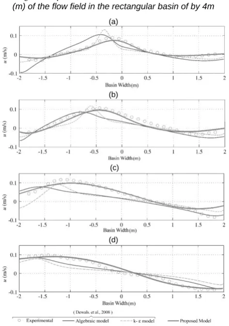
Fig. 3.Comparison between Non-dimensional moment
(m) of the flow field in the rectangular basin of by 4m
(a)
(b)
(c)
(d)
Fig. 4.Comparisons of streamwise velocities at (a) x =1.5 (b) x =2 (c) x =3 (d) x =4 m
Fig. 4 presents the measured and simulated u component of the velocity in four different cross-sections in the basin. It seems that proposed model results in determining the position and magnitude of maximum velocity is better than numerical predictions, as in [1].
VI. SENSITIVE ANALYSIS
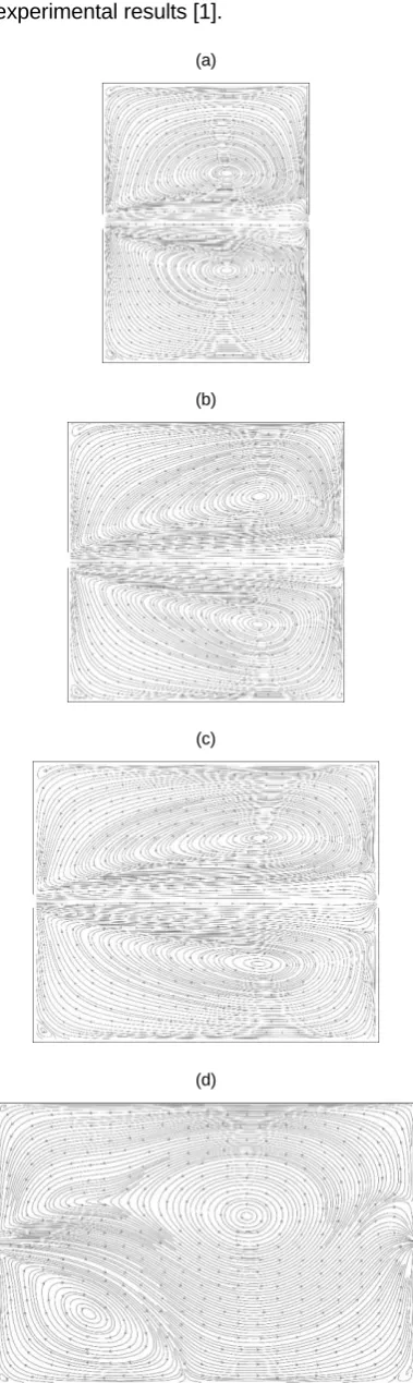
In order to determine the effects of basin length on the flow pattern, the proposed model was executed for constant basin width (4m) and different basin lengths (from 3 to 6m). As shown in fig. 5, for L/B>1.2 approximately. Flow pattern is Asymmetric. Also, for L/B≤1.2, Symmetrical flow is established.
Vol. 2 Issue 12, December - 2016
configurations lead to a non-symmetrical flow pattern, except the narrowest one, namely B = 0.5m, which is consistent with previous results. It should be noted that all of above conclusions are in agreement with experimental results [1].
(a)
(b)
(c)
(d)
Fig. 5.Flow Pattern in the basin 4m width and (a) 3m length (b) 4m length (c) 5m length (d) 6m length
To evaluate the influence of roughness coefficients on the flow patterns within the rectangular basin. The proposed model was run for three different Manning's Roughness Coefficients, n=0.007, 0.01and 0.014. The results show that Asymmetry of flow pattern decrease with the increase bed friction (see fig. 7).
(a)
(b)
(c)
(d)
Fig. 6.Flow Pattern in the basin 6m length and (a) 0.5m width (b) 1m width (c) 2m width (d) 3m width
Vol. 2 Issue 12, December - 2016
VII. CONCLUSION
The semi-lagrangian method has been applied to simulation of flow pattern in rectangular shallow basins, and the following conclusions can be drawn.
The results of proposed model have been compared with experimental and numerical models. The results show that the proposed model can predict flow pattern in rectangular basin satisfactorily. Also, investigations showed that if basin aspect ratio (length to width) was greater than 1.2, non-Symmetrical flow would establish. Otherwise, Flow pattern would be symmetric in the rectangular basin.
Finally, the effect of bed friction on flow pattern has been studied. Research indicates that Asymmetry of flow pattern decrease with the increase bed friction. However, these results may be valid only for the studied range of bed-friction values considered.
REFERENCES
[1] B.J. Dewals, S.A. Kantoush, S. Erpicum, M.
Pirotton and A.J. Schleiss, “Experimental and
numerical analysis of flow instabilities in rectangular shallow basins”,Env Fluid Mech, 8(1), pp. 31-54, 2008.
[2] Y. Peng, J. G. Zhou, and R. Burrows, “Modeling Free-Surface Flow in Rectangular Shallow Basins by Using Lattice Boltzmann Method”, Journal of Hydraulic engineering, 137(12), pp. 1680–1685, 2011.
[3] M. Dufresne, B. Dewals, S. Erpicum, P. Archambeau, M. Pirotton, “Numerical Investigation of
Flow Patterns in rectangular Shallow
Reservoirs”,Engineering Applications of
Computational Fluid Mechanics, 5(2), pp. 247-258, 2011.
[4] Clive A. J. Fletcher, “Computational
Techniques for Fluid Dynamics” Volume I, volume I of Springer Series in Computational Physics. pringer-Verla, 1991.
[5] R. Bermejo, ” On the equivalence of semi-lagrangian schemes and particle-in-cell finite element methods”, Monthly Weather Review, 118, pp. 979-987, 1990.