University of Pennsylvania
ScholarlyCommons
Publicly Accessible Penn Dissertations
1-1-2015
Essays on Macroeconometrics
Kotbee Shin
University of Pennsylvania, [email protected]
Follow this and additional works at:http://repository.upenn.edu/edissertations Part of theEconomics Commons
This paper is posted at ScholarlyCommons.http://repository.upenn.edu/edissertations/1133
For more information, please [email protected].
Recommended Citation
Shin, Kotbee, "Essays on Macroeconometrics" (2015).Publicly Accessible Penn Dissertations. 1133.
Essays on Macroeconometrics
Abstract
This dissertation presents two essays on macroeconometrics. In the second chapter, I empirically compare alternative specifications of time-varying volatility in the context of linearized dynamic stochastic general equilibrium models. I consider time variation in the volatility of structural innovations in two ways: one in which the logarithm of the volatility is assumed to follow a simple autoregressive process (stochastic volatility) and the other in which the volatility follows a Markov-switching process. A comprehensive simulation study is presented to assess the fit and performance of two specifications. I show that modeling heteroscedasticity in a highly synchronized fashion across shocks may lead to distorted estimation of the volatility. In the empirical application to the United States data, stochastic volatility model delivers the best-fit and accounts for the heteroscedasticity present in the data well.
In the third chapter, I conduct a quantitative evaluation of the potential role of adaptive expectations in a two-country dynamic stochastic general equilibrium model. Under the learning mechanism economic agents are assumed to form their expectations of forward-looking variables using a simple vector autoregressive forecasting model. The agents estimate their vector autoregression based on past model variables and update the estimates every period via a constant gain learning algorithm. I show in a simulation study that the learning mechanism increases the volatility and persistence of the endogenous variables and that as the constant gain parameter grows larger, so do these increases. The two-country DSGE model is then estimated with data from the United States and Euro area. A comparison based on log marginal data densities favors the learning over the rational expectations specification. The learning mechanism generates more persistent responses of variables to the monetary shocks. The improvement in terms of fitting the observed Dollar-Euro exchange rate dynamics is limited.
Degree Type
Dissertation
Degree Name
Doctor of Philosophy (PhD)
Graduate Group
Economics
First Advisor
Frank Schorfheide
Keywords
Adaptive Expectations, Exchange Rate Dynamics, Regime Switching Model, Stochastic Volatility, Time-varying Volatility
Subject Categories
ESSAYS ON MACROECONOMETRICS
Kotbee Shin
A DISSERTATION
in
Economics
Presented to the Faculties of the University of Pennsylvania
in
Partial Ful…llment of the Requirements for the
Degree of Doctor of Philosophy
2015
Supervisor of Dissertation
Frank Schorfheide Professor of Economics
Graduate Group Chairperson
George J. Mailath
Professor of Economics, Walter H. Annenberg Professor in the Social Sciences
Dissertation Committee
ESSAYS ON MACROECONOMETRICS
COPYRIGHT
2015
Acknowledgements
I am immensely indebted to my advisor, Frank Schorfheide. His insightful advice and
support have inspired my research and helped me strive through every stage of my
graduate studies. I am especially grateful that he has been patient with me even when
I made painfully-slow progress. I would also like to thank my dissertation committee,
Cecilia Fieler and Urban Jermann. Their valuable comments have helped shape my
research greatly. I have also bene…ted from seminar participants at the University
of Pennsylvania. I owe thanks to my undergraduate advisor, Chang-Jin Kim. His
enthusiasm in economics motivated me to become a passionate researcher.
I was so fortunate to be surrounded by smart colleagues and friends at McNeil.
I am also thankful to Kyungmin Kim, Soojin Kim, Eunice Yang, Eun-young Shim,
Cezar Santos, Dave Weiss, Chen Han, Sophie Shin, and Minchul Shin for their
friend-ship. Special thanks go to Dongho Song for substantive conversations about research.
Last and most importantly, I would like to thank my family. I cannot thank
enough to my parents and parents-in-law for their unconditional love and sacri…ce. My
deepest gratitude goes to my husband, Kihwan. Without his love and encouragement,
I could not have concluded this endeavor. Also I thank my daughter, Elyse to …ll my
ABSTRACT
ESSAYS ON MACROECONOMETRICS Kotbee Shin
Frank Schorfheide
This dissertation presents two essays on macroeconometrics. In the second
chap-ter, I empirically compare alternative speci…cations of time-varying volatility in the
context of linearized dynamic stochastic general equilibrium models. I consider time
variation in the volatility of structural innovations in two ways: one in which the
loga-rithm of the volatility is assumed to follow a simple autoregressive process (stochastic
volatility) and the other in which the volatility follows a Markov-switching process.
A comprehensive simulation study is presented to assess the …t and performance of
two speci…cations. I show that modeling heteroscedasticity in a highly synchronized
fashion across shocks may lead to distorted estimation of the volatility. In the
em-pirical application to the United States data, stochastic volatility model delivers the
best-…t and accounts for the heteroscedasticity present in the data well.
In the third chapter, I conduct a quantitative evaluation of the potential role of
adaptive expectations in a two-country dynamic stochastic general equilibrium model.
Under the learning mechanism economic agents are assumed to form their
expecta-tions of forward-looking variables using a simple vector autoregressive forecasting
model. The agents estimate their vector autoregression based on past model
vari-ables and update the estimates every period via a constant gain learning algorithm.
I show in a simulation study that the learning mechanism increases the volatility
and persistence of the endogenous variables and that as the constant gain parameter
grows larger, so do these increases. The two-country DSGE model is then estimated
data densities favors the learning over the rational expectations speci…cation. The
learning mechanism generates more persistent responses of variables to the monetary
shocks. The improvement in terms of …tting the observed Dollar-Euro exchange rate
Contents
Contents vii
List of Tables viii
List of Figures ix
I
Introduction
1
II
Regime Switching and Stochastic Volatility in DSGE
Models
4
1 Introduction 4
2 A Benchmark Model 9
2.1 Firms . . . 9
2.2 Households . . . 11
2.3 Policy . . . 14
2.4 Market Clearing . . . 14
2.5 Exogenous Stochastic Process . . . 14
2.6 Steady State and Model Solution . . . 15
3 Simulation Study 16 3.1 Simulation Design . . . 16
3.2 Model Comparison . . . 17
4.1 Estimation Approach . . . 22
4.2 Estimation Results . . . 23
5 Conclusion 27 6 Tables and Figures 28
III
Bayesian Estimation of a New Open Economy Model
with Adaptive Expectations
50
7 Introduction 50 8 The Model 53 8.1 Domestic Households . . . 548.2 Domestic Producers . . . 55
8.2.1 Domestic Final Producers . . . 55
8.2.2 Domestic Intermediate Producers . . . 58
8.2.3 Domestic Importers . . . 60
8.3 Policy . . . 61
8.4 Foreign Economy . . . 62
8.5 Market clearing . . . 64
8.6 Exogenous Stochastic Process . . . 64
9 Learning Model 65 9.1 Learning Algorithm . . . 65
9.2 Exchange Rate Determination under Learning . . . 66
11 Empirical Application 70
11.1 Posterior Distribution . . . 72
11.2 Marginal Data Density Comparison . . . 73
11.3 Impulse Response Function . . . 74
11.4 Variance Decomposition . . . 75
11.5 Posterior Predictive Checks . . . 75
12 Conclusion 76 13 Tables and Figures 77 A Appendices 90 A.1 Estimation Algorithm . . . 90
A.1.1 Stochastic Volatility in DSGE Models . . . 90
A.1.2 A Four Regime-Switching in DSGE Models . . . 94
List of Tables
1 Summary of Simulation Study . . . 28
2 Log Median Likelihood . . . 28
3 Summary of Prior Densities and Posterior Estimates . . . 29
4 Summary of Parameters for Simulation . . . 78
5 Standard Deviation of Simulated Models . . . 79
6 Correlation of Depreciation to In‡ation and Interest Rate Gap . . . . 79
7 Prior and Posterior Distribution . . . 82
8 Marginal Data Density . . . 83
List of Figures
1 True and Estimated Volatilities for the model SM1 : : : : : : : : : : : : : : 30
2 True and Estimated Volatilities for the model SM2: : : : : : : : : : : : 31
3 True and Estimated Volatilities for the model SM3: : : : : : : : : : : : 32
4 Variance Decomposition for the model SM1: : : : : : : : : : : : : : 33
5 Variance Decomposition for the model SM2: : : : : : : : : : : : : : 34
6 Variance Decomposition for the model SM3: : : : : : : : : : : : : : 35
7 True and Estimated Volatilities for the model FM1 : : : : : : : : : : : 36
8 Posterior Distributions of non-Volatility Parameters: FM1 : : : : : : 37
9 True and Estimated Volatilities for the model FM2 : : : : : : : : : : : : : 38
10 Posterior Distributions of non-Volatility Parameters: FM2: : : : : 39
11 Posterior Probability of the High Volatility Regime: FM2 : : : : : 40
12 Rolling Standard Deviations for U.S. Data: : : : : : : : : : : : : : : 41
13 Estimated Standard Deviations: SV-DSGE: : : : : : : : : : : : : : 42
14 Estimated Standard Deviations: RS(2)-DSGE: : : : : : : : : : : : : 43
15 Estimated Standard Deviations: RS(4)-DSGE: : : : : : : : : : : : : 44
16 Variance Decomposition for U.S. Data : : : : : : : : : : : : : : : : : 45
17 Posterior Probability of the High Volatility Regime: RS(2)-DSGE : : : 46
18 Posterior Probability of the High Volatility Regime: RS(4)-DSGE : : : 47
19 Posterior Probability: RS(4)-DSGE : : : : : : : : : : : : : : : : : : 48
20 Posterior Density of High- and Low- Volatility Regime Duration : : : 49
21 Autocorrelation Function of the Real Exchange Rate from Simulation 80
22 Depreciation and In‡ation, Interest Rate Gap : : : : : : : : : : : : : : 81
23 Impulse Response to U.S. Monetary Policy Shock for the Learning Model84
Model : : : : : : : : : : : : : : : : : : : : : : : : : : : : : : : : : : : : 85
25 Impulse Response to U.S. Monetary Policy Shock : : : : : : : : : : : : 86
26 Impulse Response to Euro Monetary Policy Shock : : : : : : : : : 87
27 Variance Decomposition for Depreciation in the Learning Model : : : : 88
Chapter I
Introduction
The estimation of dynamic stochastic general equilibrium (DSGE) models has been
an important subject in macroeconomics. DSGE models are useful to understand the
propagation mechanism of structural shocks to business cycle ‡uctuations and provide
a tool for the quantitative analysis of policy experiments. Over the past few decades,
there has been remarkable advance in theoretical and empirical DSGE models. DSGE
models with various frictions and di¤erent types of shocks have been developed and
they seem to reproduce the key features of data well in many dimensions. Despite the
signi…cant progress in DSGE model literature, there remains open issues on which
speci…cations DSGE model should take to characterize macroeconomic observations.
This paper aims to contribute to this literature. In this dissertation, I investigate and
empirically compare the speci…cations of DSGE models to answer two
macroecono-metric questions: (1) what is the better speci…cation between regime switching model
and stochastic volatility model to represent the overall volatility reduction, quoted as
“Great Moderation”?; (2) can adaptive expectations instead of rational expectations
explain the exchange rate dynamics in the general equilibrium framework better?
In the second chapter, I compare the regime switching models and stochastic
volatility models. Regime switching models have been a standard approach to
iden-tify the key source of a large decline in aggregate volatilities. The proponents of regime
switching approach …nd it appealing since it is a parsimonious way of modeling the
discrete jumps and can be potentially related to economic regimes with meaningful
in-terpretations. An alternative time-varying volatility model is the stochastic volatility
Stochas-tic volatility model is distinct from the regime switching model in two ways. First,
while the volatility discontinuously shifts from one level to another in the regime
switching model, it continuously changes with persistence in the stochastic
volatil-ity model. Second, the timing of volatilvolatil-ity shifts across innovations is restricted in
regime switching models, but stochastic volatility models can allow the independent
movement of volatility processes. It is of importance to take a deeper look at the
empirical performance of these two modeling approaches since a di¤erent
speci…ca-tion of variance could lead to a di¤erent conclusion on the source of macroeconomic
‡uctuations. To do so, I simulate the large-scale DSGE models with regime
switch-ing volatility and with stochastic volatility by assumswitch-ing several possible episodes of
underlying data generation processes for volatility dynamics. The simulation study
shows that the stochastic volatility speci…cation provides results comparable to or
better than regime switching models regardless of the underlying volatility patterns.
In the third chapter, di¤erent approaches to modeling the expectation formation
is explored in the open economy context. Standard open economy DSGE models
with rational expectations have had challenges in the exchange rate determination
because the exchange rates are too volatile and persistent to be justi…ed by economic
fundamentals. The empirical shortcoming of rational expectations models arise from
the tight link between the exchange rates and economic fundamentals.
Researchers have attempted to modify the open economy models with di¤erent
ingredients to relax the link of the exchange rates from the rest of the economy. In
this chapter, I focus on the expectation formation mechanism. Rational expectations
hypothesis assume that agents have complete knowledge of economic environment and
have model consistent expectations. By relaxing this strong informational
assump-tion, adaptive expectations has been of growing interest to study many
lit-erature. Under the adaptive expectations mechanism, economic agents are assumed
to form subjective expectations with limited information and learn the structure of
the economy over time. Since the agents’learning process relax the tight restrictions
on the relationships of model variables by forecast biases, the short-run dynamics of
the model variables under adaptive expectations could be substantially di¤erent from
those under rational expectations.
To quantify the role of adaptive expectations in the open economy model, I
con-duct a simulation study and estimate the model using Bayesian techniques. A
simu-lation shows that adaptive expectations mechanism increases the volatility and
per-sistence of endogenous variables and allows the exchange rates to drift away from the
uncovered interest parity equation. The estimation results provide evidence that the
adaptive expectations is a potential channel to explain the persistence of variables. I
also …nd that adaptive expectations also improve the …t of data.
Chapter II
Regime Switching and Stochastic
Volatility in DSGE Models
y
1
Introduction
In recent years, economists have produced a collection of methods to account for
heteroscedasticity present in the U.S. aggregate data. The most notable example
is the “Great Moderation” episode when the U.S. economy experienced a general
reduction in macroeconomic volatilities. A branch of macro literature has presented
empirical evidences in favor of heteroscedasticity in the shock variances. (Kim and
Nelson, 1999; McConnel and Perez-Quiros, 2000; Stock and Watson, 2002; Sensier
and van Dijk, 2004; Koopman, Lee, and Wong, 2006).
One class of time-varying models are Markov switching models. These models
allow the time series to be in any of a …nite number of distinct regimes, see Hamilton
(1989) and Kim and Nelson (1999). The choice is attractive because of the
parsimo-nious ‡exibility it provides in the speci…cation of the distributions of the underlying
structural shocks and requires fewer parameters to estimate. Markov switching
mod-els are especially appealing for characterizing the Great Moderation if there has been
a discrete and comprehensive volatility reduction in macroeconomic variables (Stock
and Watson, 2002; Chauvet and Potter, 2001; Sensier and van Dijk, 2004). Initiated
by Hamilton (1989), Markov switching models are used extensively in business cycle
analysis to characterize discrete changes in the volatilities (Sims and Zha, 2006; Davig
and Doh, 2009; Liu, Waggoner, and Zha, 2010).
A more ‡exible speci…cation is considered in stochastic volatility models, which
allow the continuous change of volatility processes having the potential for moving
one or two steps closer to complex reality. An advantage of stochastic volatility
spec-i…cation is that it can characterize continuous shifts in variance and does not restrict
the system to switch between the same con…guration. Methodologically, it is related
to the statistics literature on stochastic volatility models (Jacquier, Polson, and Rossi,
1995; Kim, Shephard, Chib, 1998; Chib, Nardari, and Shephard 2006), but the
re-cent contribution of Fernandez-Villaverde and Rubio-Ramirez (2007) and Justiniano
and Primiceri (2008) indicates that stochastic volatility in general equilibrium models
has been exploited in the business cycle literature. If the degree of time variability
di¤ers across volatility processes and the structural disturbances hitting the
econ-omy display substantial stochastic volatility, stochastic volatility speci…cation is an
e¤ective way to accommodate changes in the volatility of the U.S. economy (Cogley
and Sargent, 2005; Primiceri, 2005; Fernandez-Villaverde and Rubio-Ramirez, 2007;
Justiniano and Primiceri, 2008; Creal, Koopman, and Zivot, 2010).
While numerous studies have found signi…cant time variation in shock variances,
the magnitude, the number of structural breaks, as wells as the underlying causes of
the Great Moderation still remain as one of the main open questions in
macroeco-nomics. A lively debate unfolded between proponents of sudden change in volatility
(Stock and Watson, 2002) versus gradual reduction in volatility (Blanchard and
Si-mon, 2001). Some people are also concerned whether one or more structural breaks
exist (see the discussion in Sensier and van Dijk, 2004). However, much of the
approach. In the absence of actual knowledge of the underlying structure of volatility
processes, it is often di¢ cult to decide which estimation algorithm is the preferred
route to pursue. What is left unsaid in the literature is how model-dependent the
conclusions are when identifying the sources of macroeconomic ‡uctuations. In more
general terms, good modeling practice requires investigation of the robustness of a
conclusion when the study includes some form of economic modeling. To my best
knowledge, not much research has been done to minimize the sensitivity to
model-dependent analyses of the sources of macroeconomic ‡uctuations by estimating a
variety of structural models that assumes time-varying shock variances.
This provides a clear motivation to investigation. This paper incorporates time
varying volatility structure in large-scale linearized DSGE economies and compares
the Markov Regime-Switching (henceforth RS-DSGE) and Stochastic Volatility DSGE
(henceforth SV-DSGE) models using both simulation study and empirical application
with a strong emphasis on the speci…cation of volatility dynamics. The goal of this
paper is to provide a systematic examination of the performance of two competing
models in explaining the driving sources of macroeconomic ‡uctuations.
Investiga-tion is important since macroeconomic implicaInvestiga-tions can be seriously distorted if the
competing models produce di¤erent volatility estimates. First, I investigate whether
the outcomes of two models are similar and second, which model is more reliable. I
believe that only after taking account of the model sensitivity, it is possible to draw
a …rm conclusion about the sources of macroeconomic ‡uctuations. This paper also
tries to address the danger of relying exclusively on a model selection criterion that
favors models that …t the data well. A common practice in the empirical DSGE
lit-erature is comparing models using marginal likelihood. From a Bayesian perspective,
the marginal data density is the most comprehensive and accurate measure of …t and
aid of simulation examples and empirical application that a situation where volatility
dynamics are spuriously estimated but it survives the Bayesian model selection
crite-rion for o¤ering a parsimonious approximation and delivering a better time-series …t
is possible
I propose a simulation study. The architecture of simulation study is designed to
replicate salient features of U.S. business cycles and is implemented by using arti…cial
dataset of 200 observations generated using a large scale DSGE model of Justiniano
and Primiceri (2008) (henceforth, JP). The details are discussed in Section 3.
Applica-tion to the simulated dataset will provide guidance on how well each competing model
performs when the true model is in hand. In a simulation study, model performances
are measured in three di¤erent ways. I compare the estimated volatility components
to the true Data Generating Process (henceforth DGP), perform variance
decompo-sition to examine the consequence of volatility misspeci…cation, and compute the log
marginal data density to measure the data …t. Next, I repeat the same steps with
the aggregate U.S. data and use the simulation results as a benchmark to understand
and interpret the empirical performance of each model.
The main empirical …ndings in the experiments are as follows. A two
regime-switching DSGE (henceforth, RS(2)-DSGE) model seems inappropriate for drawing
inferences about the volatility processes of business cycles. A common disadvantage of
RS(2)-DSGE models is that they assume complete synchronization of Markov states
across volatilities. Estimated volatilities can be very crude if the true DGP exhibits
contrasting patterns of ‡uctuations. The natural step is to amend RS(2)-DSGE to
allow additional degree of ‡exibility in the movement of volatilities. A four
regime-switching DSGE (henceforth RS(4)-DSGE) model nests RS(2)-DSGE in this regard.
Hence, I argue that RS(4)-DSGE may perform better than RS(2)-DSGE model for
provid-ing extra degree of ‡exibility in the RS-DSGE model is a challengprovid-ing task. SV-DSGE
model, on the contrary, promises great ‡exibility in modeling volatility dynamics and
its performance is certainly not inferior to RS-DSGE’s. However, the price for this
‡exibility is an increase in dimension. Aside from the over-parametrization
prob-lem, SV-DSGE estimates may exaggerate or discount time variation and stochastic
movement in volatility. Its performance may deteriorate as the oscillation between
volatility regimes increases and the di¤erence between the regimes decreases.
In the application to U.S. aggregate data, I estimate the large scale DSGE model
in JP using RS(2)-DSGE, RS(4)-DSGE, and SV-DSGE models. I have grouped a
subset of shock variances having the same Markov processes. I allow regime
associ-ated with the variances of the monetary policy shock to be independent of the regime
switching processes of the other shock variances. The empirical motivation is from
Sensier and van Dijk (2004) and Cecchetti, Hooper, Kasman, Schoenholtz, and
Wat-son (2007) that the volatility of in‡ation has undergone multiple structural breaks. I
…nd that SV-DSGE model delivers a best-…t and accounts for the heteroscedasticity
present in the data well. RS(4)-DSGE performs better than RS(2)-DSGE model in
volatility speci…cation, but does not improve upon the data …t. By synchronizing
shifts in variances across two regimes, RS(2)-DSGE model may detect the timing of
the volatility regime wrong and provide imprecise estimates for volatility processes
while …tting to the data better than RS(4)-DSGE model. In order to provide
robust-ness of empirical …ndings, I perform the variance decomposition and compute the
marginal data density using the modi…ed harmonic mean method of Geweke (1999).
Liu, Waggoner, and Zha (2010) is the closest paper to ours. They examine the
sources of macroeconomic ‡uctuations by estimating a number of alternative
regime-switching models using Bayesian methods in a uni…ed DSGE framework and compare
density and Schwarz criterion, they …nd strong evidence in favor of the RS(2)-DSGE
model where regime shifts in the variances are synchronized. They then use
RS(2)-DSGE model to identify shocks that are important in driving macroeconomic
‡uctu-ations. My approach di¤ers from Liu et al. (2010) since I extend the investigation by
including stochastic volatility speci…cation and examine the e¤ectiveness of Bayesian
model-selection criterion.
This chapter is organized as follows. Section 2 brie‡y explains the DSGE model
framework, Section 3 constitutes a simulation study. Section 4 illustrates an
applica-tion to U.S. aggregate data and Secapplica-tion 5 concludes. Technical details are summarized
in Appendix.
2
A Benchmark Model
The model is based on JP and exhibits a number of real and nominal rigidities which
has been shown to …t the data fairly well. For additional details, see JP. The basic
elements of the model include a continuum of households, perfectly competitive …nal
goods producers, and a continuum of monopolistic intermediate goods producers.
Monetary policy follows a Taylor type rule and …scal policy is assumed to be fully
Ricardian. Here is the illustration of the JP model.
2.1
Firms
A monopolistic intermediate goods producing …rm i2[0;1]produces output
accord-ing to:
whereAtis an exogenous measure of productivity that is the same across …rms and F
represents a …xed cost of production. As usual, Kt(i) and Lt(i) denote, respectively,
the capital and labor input for the production of good i. Atfollows a unit root process,
with a growth rate (zt logAAtt1) that follows:
zt= (1 z) + zzt 1+ zt"zt (1)
Firms follow a Calvo pricing mechanism when they set their prices. At the start
of each period, a randomly selected fraction p of …rms cannot reoptimize and set
their prices according to:
Pt(i) =Pt 1(i) tp1
1 p
where tis de…ned as PPt
t 1 and is the steady-state value. Remaining fraction 1 p of …rms choose their prices by maximizing the present value of future pro…ts:
Et 1 X s=0 s p s t+s
n
[Pet(i)( sj=0
p
t 1+j
1 p)]Y
t+s(i) [Wt+sLt+s(i) +Rkt+sKt+s(i)]
o
where t+sis the marginal utility of consumption, andWtandRtkdenote, respectively,
the wage and the rental cost of capital.
There is a representative …nal goods producing …rm that produce the
consump-tion goods using the intermediate goods and the following constant-returns-to-scale
technology:
Yt=
2 4
1 Z
0 Yt(i)
1 1+ ptdi
3 5
1+ pt
where pt follows the exogenous stochastic process
Pro…t maximization problem for the …nal goods producer yields a demand for each
intermediate good given by
Yt(i) =
Pt(i) Pt
(1+ pt)
pt
Yt
and the zero pro…t condition imply
Pt =
2 4
1 Z
0 Pt(i)
1 ptdi 3 5 pt :
2.2
Households
Firms are owned by a continuum of households, indexed byj 2[0;1]:As in JP, while
each household is a monopolistic supplier of specialized labor, a number of
"employ-ment agencies" combine households’specialized labor into labor services available to
the intermediate …rms:
Lt=
2 4
1 Z
0 Lt(j)
1 1+ wdj
3 5
1+ w
Pro…t maximization problem for the employment agencies yields a demand for each
labor given by
Lt(j) =
Wt(j) Wt
(1+ w)
w
Lt
and the zero pro…t condition imply
Wt=
2 4
1 Z
0
Wt(j)
Household j’s preferences are representable by a lifetime utility functions:
Et 1
X
s=0 s
bt+s log(Ct+s(j) hCt+s 1(j)) 't+s
Lt+s(j)1+
1 +
which is separable in consumption, Ct(j); and labor Lt(j): h is the degree of habit
formation, 't is a preference shock that a¤ects the marginal disutility of labor, and
bt is a discount factor shock a¤ecting both marginal utility of consumption and the
marginal disutility of labor. Both shocks follow exogenous stochastic processes
logbt= blogbt 1+ bt"bt (3)
log't = (1 ') log'+ 'log't 1+ 't"'t: (4)
The jth household’s budget constraint is given by:
Pt+sCt+s(j) +Pt+sIt+s(j) +Bt+s(j) Rt+s 1Bt+s 1(j) +Qt+s 1(j) + t+s
+Wt+s(j)Lt+s(j) +Rkt+s(j)ut+s(j)Kt+s 1(j) Pt+sa(ut+s(j))Kt+s 1(j)
whereIt(j)is investment, Bt(j)denotes government bonds holding, Rt is gross
nom-inal interest rate, Qt(j) is the net cash ‡ow from participating in state contingent
securities, and t is the per capita pro…t that households get from owing the …rms.
Households own capital and choose the capital utilization rate that transforms
phys-ical capital Kt(j) into e¤ective capital
Kt(j) =ut(j)Kt 1(j);
which is rented to …rms at the rateRk
per unit of physical capital. Following JP, I assume ut = 1 and a(ut) = 0 in steady
state. In this partially nonlinear approximation of the model solution, only the
cur-vature of the function in steady state needs to be speci…ed, = aa000(1)(1): The usual physical capital accumulation equation is described by
Kt(j) = (1 )Kt 1(j) + t(1 S( It(j) It 1(j)
))It(j);
where denotes the depreciation rate and S captures the investment adjustment
cost, with S0 > 0 and S00 > 0.
t can be interpreted as an investment-speci…c
technology shock following Greenwood, Hercowitz, and Krusell (1997). Assume that
this investment shock follows the exogenous stochastic process
log t = log t 1 + t" t: (5)
Households follow a Calvo pricing mechanism when they set wages. At the start
of every period, a randomly selected w of households cannot reoptimize wages and
set their wages according to the indexation rule:
Wt(j) = Wt 1(j)( t 1ezt 1)w( e )1 w:
The remaining 1 w of households set their wages by maximizing
Et 1
X
s=0 s w
s
bt+s 't+s
Lt+s(j)1+
1 +
subject to
Lt(j) = Wt(j)
Wt
(1+ w)
w
2.3
Policy
The monetary authority sets the short-term nominal rate using the following rule
Rt R = (
Rt 1
R )
R ( t) (Yt=At
Y =A )
Y
1 R
e Rt"Rt; (6)
whereRis the steady state for the gross nominal interest rate and"Rtis a monetary
policy shock.
Fiscal policy is, by assumption, fully Ricardian, and public spending is given by
Gt= (1
1
gt
)Yt
where gt is an exogenous disturbance following the exogenous stochastic process
loggt= (1 g) logg+ gloggt 1+ gt"gt: (7)
2.4
Market Clearing
The resource constraint is given by
Ct+It+Gt+a(ut)Kt 1 =Yt
2.5
Exogenous Stochastic Process
With regard to exogenous stochastic process in (1)-(7), "jt~iidN(0;1) where j 2
fz; p; b; '; ; R; gg and t denotes time: As for the standard deviations, j , I assume
models: For instance, 2 fHigh volatility regime; Low volatility regimeg in two
Markov regime-switching model. Following Kim, Shepard, and Chip (1998), I assume
that each element of jt evolves independently according to the following stochastic
processes:
log jt = (1 j) log j+ jlog jt 1+ jt
jt~iidN(0; !2j)
2.6
Steady State and Model Solution
Since technology process At is a unit root process, after detrending consumption,
investment, capital, real wages, and output, I are able to compute the
nonsto-chastic steady state. De…ne the vector of relevant model endogenous variables t.
Solution of the linear rational expectations system, Et[f( t+1; t; t 1; t; )] = 0;
where t is a vector of exogenous disturbances and is a vector of structural
para-meters, is obtained by running Chris Sims’s code gensys.m. Then, the observable
yt = [4logYt;4logCt;4logIt;logLt;4logWt
Pt; t; Rt] can be expressed as a linear
function of the endogenous model variables xt
yt =D+Z t (ME)
t=T( ) t 1+R( ) t (TE)
3
Simulation Study
3.1
Simulation Design
In this section I propose a simulation study for the performance evaluation of
RS(2)-DSGE, RS(4)-RS(2)-DSGE, and SV-DSGE model.
I consider three simulation scenarios in which the key qualitative features of the
Great Moderation are replicated. In the …rst set of simulation, labeled as SM1,
whereas monetary shock displays a double shaped pattern. A double
hump-shaped pattern of monetary shock has its ground in the growing literature on Markov
switching DSGE models (see, for more information, Davig and Doh, 2009; Bianchi,
2010; Liu, Waggoner, and Zha, 2010). All other structural shocks exhibit a one time
permanent reduction in the volatility. Many empirical studies document a discrete
drop in conditional variance of macroeconomic time series. For example, Stock and
Watson (2002) argue that changes in the volatility around 1984 are comprehensive
and best characterized as discrete break. The second simulation scenario (henceforth,
SM2) complexi…es volatility process one step further by allowing a subset of volatilities
to have independent regimes. By doing so, I are able to examine the ability of each
estimation method to recover the true volatility speci…cation. The last simulation
scenario (henceforth, SM3) is based on the argument that the high volatility regime
is often associated with recession (French and Sichel, 1993; Hamilton and Susmel,
1994). Since there are relatively fewer number of recessions after 1990s, this may
appear as volatility reduction. I let high volatility regimes manifest themselves at the
NBER recession dates.
In all scenarios, I assume the true DGP to follow Markov processes since the
volatility dynamics can be easily con…gured to replicate salient features of Great
a simulation study I shut down Metropolis-Hastings algorithm and give the true
para-meter values for non-volatility parapara-meters. A full-blown estimation requires roughly
three (two) days to complete 200,000 iteration for RS-DSGE (SV-DSGE) models
which is the minimum of iteration number to achieve convergence. Since I are
in-terested in the estimation of volatility dynamics, without loss of generality, I assume
true values for non-volatility parameters are recovered through Metropolis-Hastings
algorithm. All simulations are based on arti…cial dataset generated from a large scale
DSGE model of JP and the posterior median estimates for non-volatility parameters
in JP are used.
Next, I conduct some full-blown estimation to check the validity of the
assump-tion that true values for non-volatility parameters are recovered through
Metropolis-Hastings algorithm. I extend SM1 to a full-blown estimation scheme and denote as
FM1. I also consider a case (henceforth, FM2) in which the true DGP follows
sto-chastic volatility process. Here, I use the posterior volatility estimates of SV-DSGE
in JP as DGP and try to estimate with RS(2)-DSGE model. This exercise centers
on the following idea: if the true DGP of macroeconomic variables follow stochastic
volatility process, how well RS(2)-DSGE models estimate the volatility dynamics?
Table 1 summarizes the simulation study.
3.2
Model Comparison
Model performance is measured in three di¤erent ways; I compare the estimated
volatility components to the true DGP, perform variance decomposition to examine
the consequence of volatility misspeci…cation, and compute the log marginal data
density to measure the data …t. All …gures are obtained from the remaining 10,000
plot the time-varying standard deviations for the structural shocks of each model. Top
panels of …gure 1, …gure 2 and …gure 3 juxtapose the volatility estimates from
RS(4)-DSGE, SV-DSGE model, and true DGP. Bottom panels are constructed similarly
but carry the estimates from RS(2)-DSGE model. Figure 4 to …gure 6 present the
evolution of the variance shares of GDP growth attributed to each structural shock.
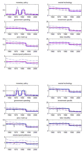
Figure 1 is based on SM1. Note that the true DGP and the estimates from
RS(4)-DSGE model are almost identical in the top panel. However, in the bottom
panel, the estimated monetary shock demonstrates a one-time reduction in volatility
as the other shocks do. This is inevitable because RS(2)-DSGE assumes all shock
variance to switch regimes simultaneously. Due to limited space, I do not report in
this paper but depending on the parameterization, I have cases where all estimated
shock variances follow a double hump-shaped. This double hump-shaped pattern
has been consistently documented in previous literatures (see Davig and Doh, 2009;
Bianchi, 2010; Liu, Waggoner, and Zha, 2010). From this example, I cast doubt on the
estimated volatility components from the RS(2)-DSGE model. I believe that when
the model assumes synchronized regime shifts in the variances, it is more likely to
produce spurious estimates. SV-DSGE model captures the time variation in volatility
well.
Some interesting …ndings are shown in …gure 2. I slightly modify SM1 by allowing
independent regimes for government spending and price mark-up shocks. It is now
called SM2. The estimates from RS(2)-DSGE, presented in the bottom panel, are
misleading in that they spuriously detect the number of structural breaks in volatility.
They can be very crude as the true DGP exhibits contrasting patterns of ‡uctuations.
Considering that the number of structural breaks in macroeconomic time series is still
controversial, this result deserves attention. RS(4)-DSGE allows additional degree of
volatility movements than RS(2)-DSGE. One remark is that when grouping a subset
of shock variances to have the same Markov processes, I have to rely on empirical
evidences to …nd the right combination. I will discuss this in more detail in the
application to real data.
A common disadvantage of RS-DSGE models is that they assume perfect
syn-chronization of Markov states across volatilities. SM1 and SM2 show how easily
RS-DSGE model can be misleading when the evolutions of shock volatilities are
sep-arated. On the other hand, SV-DSGE performs quite well in both scenarios. Since
I employ random-walk speci…cation for the stochastic volatility processes, SV-DSGE
can account for both a gradual decline and a sudden change in volatility.
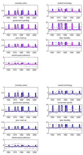
In SM3, I try to identify cases when SV-DSGE model performs poorly as shown in
…gure 3. SV-DSGE estimates may exaggerate or discount time variation in volatility.
Because SV-DSGE has a tendency to smooth out the patterns, when there are
fre-quent oscillations the estimates can be misleading. I do not report in this paper, but
when the di¤erences between the two volatility regimes are small, the posterior
cred-ible interval of SV-DSGE widens and the time-invariant volatility hypothesis cannot
be rejected.
What can go wrong if the estimated volatility processes are misspeci…ed? I would
like to address this issue by performing variance decomposition. This exercise is
important since conclusions drawn from the estimated volatility components are
de-pendent on the estimation methods and consequently variance decomposition results
will di¤er. Variance decomposition is obtained by solving the following discrete
Lya-punov equations:
V ar( tj ; Qt) = T( )V ar( tj ; Qt)T( )0+R( )QtR( )
whereQtis a regime-dependent variance-covariance matrix in RS-DSGE and is per se
a stochastic volatility variance-covariance matrix in SV-DSGE. The contribution of
shockiis obtained by setting to zero the volatility of all disturbances but one, 2 it:
Fig-ure 4 through FigFig-ure 6 report the evolution of the variance shares of GDP growth
at-tributed to each structural shocks. Variance decomposition results are mostly similar
across models. Especially, SV-DSGE and RS(4)-DSGE models produce qualitatively
similar results in all scenarios. However, SV-DSGE model slightly exaggerates the
role of government spending shock in explaining the variability of GDP growth. The
variance decomposition from RS(2)-DSGE relies on the poorly estimated volatilities
and tend to exaggerate the role of monetary policy shock.
Table 2 reports the log likelihood for all combination of experiments. Since my
simulation study shut down Metropolis-Hastings algorithm for non-volatility
parame-ters, I use log median likelihood in model comparison. Note that I am integrating
out the unobserved volatilities nor penalizing the likelihood with the number of
para-meters, instead I computeL(Yjvolatilities; true non-volatility parameters). Although
this approach will favor models with many parameters, it may be a primitive way to
understand the e¤ectiveness of each model. I use marginal data density approach in
the empirical application. SV-DSGE model outperforms others with the exception of
SM3. RS(2)-DSGE model performs poorly in general, but if there is a synchronized
regime switching in shock volatility, RS(2)-DSGE model is the best-…t model. Note
that the performance of RS(4)-DSGE model is certainly better than RS(2)-DSGE
model in all scenarios. SV-DSGE model delivers best-…t in two out of three scenarios
that I considered.
In sum, I argue that when there is not enough knowledge about the volatility
process, RS(2)-DSGE model may not be a good choice since it cannot minimize the
allowing for additional degree of ‡exibility can cure this problem. SV-DSGE model
can be a good candidate since it promises great ‡exibility in modeling volatility
dynamics and delivers data-…t.
A Full-blown Estimation I report the …ndings from a full-blown estimation. Two sets of full-blown estimations are conducted by generating 200,000 draws. All
…ndings are reported after discarding the initial 150,000 posterior draws. First, I
modify the estimation algorithm to make inferences about the non-volatility
para-meters in SM1 setting. Notice that volatility estimates from SV-DSGE in …gure 7
are very similar to those in …gure 1. Estimation of non-volatility parameters does
not change the inference of volatility processes. Figure 8 shows the kernel density
estimation of Bayesian posterior distributions of non-volatility parameters. Except
few parameters, the Bayesian credible set includes the true values.
Second, I use the posterior median estimates of volatility processes from JP as
the true DGP and estimate with RS(2)-DSGE model. Figure 9 plots the estimated
time-varying volatility components. As suggested in the simulation study,
RS(2)-DSGE model detects spurious structural break in some volatility components. This
is because regime shifts in the variances are synchronized. Figure 10 shows the kernel
density estimation of Bayesian posterior distributions of non-volatility parameters.
Compared to …gure 8, more true parameter values is not contained in the Bayesian
credible set. It is not clear at this point what roles volatility speci…cations play in
consistent estimation of non-volatility parameter values. It might be that volatility
misspeci…cation a¤ects Kalman gain and in turn compromises the validity of the
Kalman …lter. Figure 11 displays the posterior expected values of the high-volatility
4
Application to U.S. data
4.1
Estimation Approach
I estimate SV-DSGE, RS(2)-DSGE, and RS(4)-DSGE using the same prior
distrib-utions and dataset in JP 2008. The data comprises of seven series of U.S. quarterly
aggregate variables; the growth rate of output, consumption, investment, real wage,
the log of hours worked, annualized in‡ation, and nominal interest rates (for more
details on data description, see JP 2008). I use the same priors for non-volatility
parameters across three speci…cations in order to treat them equal a priori. I refer
to Liu, Waggoner, and Zha (2010) for the choice of the prior distributions for the
volatility parameters.
As discussed previously, a careful investigation is required to determine how to
group a subset of shocks. I allow regime associated with the variance of monetary
policy shock to be independent of the regime switching processes of the other shock
variances based on previous literatures and on the rolling estimation of standard
deviations presented in …gure 12. Sensier and van Dijk (2004) …nd that 83% of the U.S.
macroeconomic time series variables have experienced a break in the (un)conditional
volatility, and in particular nominal variables such as in‡ation and interest rates
experienced multiple volatility breaks. Cecchetti et al. (2007) report that the level
and volatility of in‡ation display coincident hump-shaped patterns that allow us to
date the start of the Great In‡ation in the late-1960s and a synchronized In‡ation
Stabilization in the mid-1980s. The rolling estimation of standard deviations in …gure
12 depicts the overall volatility movements. Consistent with Cecchetti et al. (2007), I
also witness multiple ‡uctuations in two nominal variables, in‡ation and interest rates.
This motivates us to assume that the regime associated with nominal shock variances
here on, I denote RS(4)-DSGE as the model with the regime associated with monetary
shock being independent of other regimes.
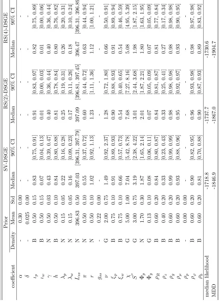
Table 3 reports posterior medians and …fth and ninety-…fth percentiles of a model
estimated with SV-DSGE, RS(2)-DSGE, and RS(4)-DSGE model. All posterior
esti-mates are obtained by running a single block random-walk MH algorithm (RW-MH)
for 400,000 iterations following a burn-in of 350,000 iterations. Calibrated
para-meters are capital share ( ) at 0.3, depreciation rate ( ) at 0.025, SS government
spending share (g) at 0.22, and persistent of mark-up shock ( ) at zero. Chib and
Ramamurthy (2010) argue that the results from the RW-MH algorithm are not
sat-isfactory due to slow convergence and often the algorithm does not work in many
circumstances. According to Sims, Waggoner, and Zha (2008), due to the complexity
inherent in high-dimensional Markov-switching models, the RW-MH algorithm can
be very costly and sometimes take a couple of weeks to obtain an estimate that is
close to the peak of the likelihood. Indeed, RW-MH algorithm needed around …ve
days to complete 400,000 iterations for RS-DSGE models. I assess the convergence of
RS-DSGE model using some di¤erent starting values and found that they delivered
roughly similar results when looking at medians. However, due to substantial
compu-tational burden, the (informal) convergence test was limited. For SV-DSGE model, I
veri…ed the robustness of the algorithm by obtaining almost identical posterior median
values in JP 2008.
4.2
Estimation Results
Parameter estimates are not entirely identical. While most of the parameter
esti-mates from SV-DSGE are similar to ones reported in JP 2008, labor-related
parameters of RS-DSGE models are somewhat di¤erent. For example, labor disutility
coe¢ cient is higher in both RS(2)-DSGE and RS(4)-DSGE models. This may
some-how generate lower labor disutility shock estimates than one from SV-DSGE model.
Although this variation in estimates may be important, I do not explore it any more.
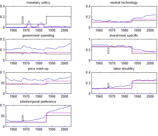
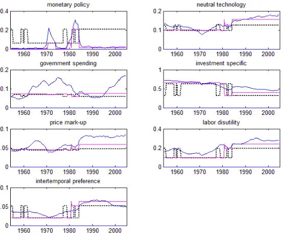
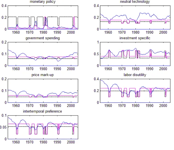
Instead, I would like to focus on volatility estimates. Figure 13 through …gure 15 plot
the time-varying standard-deviations for the seven structural shocks of SV-DSGE,
RS(2)-DSGE, and RS(4)-DSGE models, respectively. Note that …gure 13 is roughly
identical to the results in JP 2008. In …gure 14, observe that the estimates of
mone-tary policy, investment speci…c, and government spending shocks are roughly similar
to those in SV-DSGE model, but the estimates of technology and intertemporal
pref-erence shocks behave very di¤erently. While these two estimates from SV-DSGE
model tend to show gradual decline over the time periods, corresponding estimates
from RS(2)-DSGE model are characterized by multiple Markov-shifts. Since the true
volatility process is unknown, I do not know which is closer to the truth. However,
it is very unlikely that all volatility processes change magnitude and shape
simul-taneously. The estimates from RS(4)-DSGE model look quite similar to those from
RS(2)-DSGE model. But two things stand out in …gure 15. Since I allow the regime
associated with the exogenous disturbance showing the largest degree of time
varia-tion (monetary policy shock) to be independent of the regime switching processes of
other shock variances, the double-hump shaped pattern is most notable in monetary
policy shock estimates. Also, relatively fewer high volatility regimes are realized since
mid 1980s. This enables us to replicate the great reduction in volatility of the
remain-ing disturbances around mid 1980s. The fact that estimates from RS(2)-DSGE and
RS(4)-DSGE models are somewhat di¤erent indicates that independent movement
across volatility processes are evident. This shows why one should be careful about
U.S. macroeconomic variables.
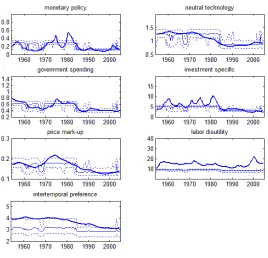
Figure 16 presents the variance decomposition for output growth. With some
exception, each model delivers roughly similar results. Note that SV-DSGE model
assumes variance shares attributed to each shock are more time-varying. Figure 17
and …gure 18 show posterior expected values of the high volatility regime in
RS(2)-DSGE and RS(4)-RS(2)-DSGE model. Notice that …gure 17 looks as if the two posterior
expected values in Figure 18 are combined in one …gure. According to RS(2)-DSGE
model, the high volatility regimes for monetary shock are observed in the mid-1960s
and in the beginning of 2000s. (See also the …gure 2 in Liu, Waggoner, and Zha (2010),
page 40. They have the same …gure like I do.) Figure 18 tells us that there was no high
volatility regime for monetary shock at that time. Observe that the starting period
of high volatility regime for monetary shock and that for the others do not coincide
in early 2000s. By allowing additional degree of ‡exibility in RS-DSGE model, I am
able to detect the timing of each volatility regime shift better. Figure 19 separately
plots the regime probabilities in RS(4)-DSGE model. The second and third rows in
Figure 19 imply that taking account of these two possible regimes can be important
since both of them are signi…cantly greater than zeros in probabilities.
I try to address the drawback of RS(2)-DSGE model in di¤erent direction. Using
the posterior median values of SV-DSGE model, reported in Table 3 and …gure 13, I
generate an arti…cial dataset. The thought experiment centers on the following idea:
provided that SV-DSGE model ideally captures the volatility dynamics, how is the
performance of RS(2)-DSGE model. Figure 13 is now used as the true DGP and
the estimates of monetary shock disturbance in the …gure tell us that low volatility
regime was present in the mid 1960s. However, the estimates from RS(2)-DSGE
model detects the presence of high volatility regime for monetary shock at that period.
displayed in …gure 11. This …gure conveys wrong impression that monetary shock was
in high volatility state around 1960s as well as other shocks. These evidences show
that RS(2)-DSGE model can detect the timing of the high volatility regime wrong
and provide imprecise estimates for volatility processes.
As it is standard in the literature, I assess the …t by computing the marginal data
density as suggested in Geweke (1999). From a Bayesian point of view, the
mar-ginal data density comparison gives a comprehensive measure of …t on non-nested
competing models. Details of the computation of the marginal data density is
rel-egated to the technical appendix in JP 2008. However, I would like to point out
that JP do not integrate out all latent variables numerically. In fact, JP choose
f( ; HT) =f( )f(HT) = f( ) (HT) and assume ( ; HT) = ( ) (HT) for
compu-tational convenience:
m(Y) =
Z f( ; HT)
L(Yj ; HT) ( ; HT)p( ; H T
jY)d( ; HT) 1
Then, the marginal data density can be approximated by:
mN(Y) =
" 1
N N
X
j=1
f( j) p(Yj j; HjT) ( j)
) # 1
where j and HjT are from posterior distribution. I acknowledge the possible
approx-imation error from following JP’s method. But, at the same time I understand that
their assumption allows us to computemN(Y)very easily.
The last two rows of Table 3 reports the log-marginal data density and the median
likelihood values for SV-DSGE, RS(2)-DSGE, and RS(4)-DSGE model, respectively.
Consistent with JP, I …nd that the values of the log-marginal likelihood are in favor
that between the two speci…cations of RS-DSGE models, the data favor the
parsimo-niously parameterized model with shock variances switching regimes simultaneously.
I suspect that volatility dynamics are spuriously estimated in RS(2)-DSGE model but
…nd out that it performs pretty well in terms of the Bayesian model selection criterion
for o¤ering a parsimonious approximation and delivering a better data …t.
Consis-tent with the simulation study, I …nd that the median likelihood value for SV-DSGE
model is the highest while RS(4)-DSGE model is the lowest.
5
Conclusion
I have estimated a variety of large-scale DSGE models in which the variance of
the structural shocks is time-varying. In particular, I evaluated the e¤ectiveness
of Markov-switching and stochastic volatility speci…cation of volatility dynamics.
Re-sults from simulation indicate that allowing for too few regimes in the RS-DSGE
model leads to poor volatility estimates. SV-DSGE model promises great
‡exibil-ity in modeling volatil‡exibil-ity dynamics in a sense that it does not restrict the number
of changes nor synchronization across shocks. In empirical application, SV-DSGE
model delivers best-…t and accounts for the heteroscedasticity present in the data
well. Among RS-DSGE models, the one with synchronized shifts in shock variances
…ts best, but may provide imprecise estimates for volatility processes. I have shown
that model comparison based on the marginal likelihood approach can be
mislead-ing since parsimoniously parameterized model will always be favored regardless of
its ability to capture volatility dynamics. The …ndings imply that DSGE models
extended with stochastic volatility are good alternatives for understanding the
evolv-ing volatility dynamics of U.S. aggregate data since it can minimize the impact of
6
Tables and Figures
Table 1: Summary of Simulation Study
Description True DGP Estimation SM1 Monetary vs the Rest RS(4) Restricted+
SM2 Monetary vs Gov’t and Price Mark-up vs the Rest RS(8) Restricted+
SM3 High volatility in recession RS(2) Restricted+
FM1 Monetary vs the Rest RS(4) Full-blown FM2 Stochastic Volatility Process SV Full-blown
Note. Restricted+: I only estimate volatility parameters.
Table 2: Log Median Likelihood
DGPnEstimation RS(2)-DSGE RS(4)-DSGE SV-DSGE SM1 -1892.25 -1793.39 -1783.69 SM2 -1823.29 -1729.91 -1710.28
Figure 1: True and Estimated Volatilities for the model SM1
Note: In this …gure I plot the true volatility processes (bold), median standard deviation and 90%
credible intervals generated in the estimation of SV-DSGE (dashed), RS(2)-DSGE (black-dotted),
Figure 2: True and Estimated Volatilities for the model SM2
Note: In this …gure I plot the true volatility processes (bold), median standard deviation and 90%
credible intervals generated in the estimation of SV-DSGE (dashed), RS(2)-DSGE (black-dotted),
Figure 3: True and Estimated Volatilities for the model SM3
Note: In this …gure I plot the true volatility processes (bold), median standard deviation and 90%
credible intervals generated in the estimation of SV-DSGE (dashed), RS(2)-DSGE (black-dotted),
Figure 4: Variance Decomposition for the model SM1
Note: This …gure presents the contribution of each shock to the variability of GDP growth.
Vari-ance decomposition under RS(4)-DSGE (pink), SV-DSGE (blue), and RS(2)-DSGE model
Figure 5: Variance Decomposition for the model SM2
Note: This …gure presents the contribution of each shock to the variability of GDP growth.
Vari-ance decomposition under RS(4)-DSGE (pink), SV-DSGE (blue), and RS(2)-DSGE model
Figure 6: Variance Decomposition for the model SM3
Note: This …gure presents the contribution of each shock to the variability of GDP growth.
Vari-ance decomposition under RS(4)-DSGE (pink), SV-DSGE (blue), and RS(2)-DSGE model
Figure 7: True and Estimated Volatilities for the model FM1
Notes: Bold lines represent true volatility processes. Median standard deviations(solid) and 90%
Figure 8: Posterior Distributions of non-Volatility Parameters: FM1
Note: This …gure plots kernel density estimation of posterior distributions. True parameter
Figure 9: True and Estimated Volatilities: FM2
Notes: Bold lines represent true volatility processes, SV-DSGE. Median standard deviations
Figure 10: Posterior Distributions of non-Volatility Parameters: FM2
Note: This …gure plots kernel density estimation of posterior distributions. True parameter
Figure 11: Posterior Probability of the High Volatility Regime: FM2
Notes: Shaded bars indicate NBER recessions and solid line represents posterior expected value
of the high volatility regime in DSGE model. DGP is SV-DSGE and I estimate with
Figure 12: Rolling Standard Deviations for U.S. Data
Figure 13: Estimated Standard Deviations: SV-DSGE
Notes: Median (bold) and 90% credible intervals (dotted) for the time-varying volatility of each
Figure 14: Estimated Standard Deviations: RS(2)-DSGE
Notes: Median (bold) and 90% credible intervals (dotted) for the time-varying volatility
of each disturbance computed with the draws generated in the estimation of RS(2)-DSGE
Figure 15: Estimated Standard Deviations: RS(4)-DSGE
Notes: Median (bold) and 90% credible intervals (dotted) for the time-varying volatility of each
Figure 16: Variance Decomposition for U.S. Data
Notes: This …gure presents the contribution of each shock to the variability of GDP growth.
Vari-ance decomposition under RS(4)-DSGE (pink), SV-DSGE (blue), and RS(2)-DSGE model
Figure 17: Posterior Probability of the High Volatility Regime: RS(2)-DSGE
Notes: Shaded bars indicate NBER recessions and solid line represents posterior expected value
of the high volatility regime in RS(2)-DSGE model. The results are based on 300,000 posterior
Figure 18: Posterior Probability of the High Volatility Regime: RS(4)-DSGE
Notes. Solid line represents posterior probability of the high volatility regime for monetary shock
Figure 19: Posterior Probability: RS(4)-DSGE
Notes: Shaded bars indicate NBER recessions and bold lines are posterior probability of each
Figure 20: Posterior Density of High- and Low- Volatility Regime Duration
Notes: Top …gure is posterior density of each regime for RS(2)-DSGE and two bottom …gures
Chapter III
Bayesian Estimation of a New
Open Economy Model with
Adaptive Expectations
7
Introduction
Explaining real exchange rate dynamics has been an long-lasting challenge in
inter-national economics. Exchange rates are more volatile and persistent than standard
open-economy models can account for, and they appear to be disconnected from
fun-damentals in the short run. In one strand of the literature, there are a large number of
theoretical studies which incorporate the endogenous sources that can make
consump-tion unresponsive to the exchange rate. Some examples include nominal rigidities,
pricing-to-market, introduction of durable goods and investment, and alternative
as-set market structure, e.g., the work of Betts and Devereux (2000), Chari, Kehoe and
MaGrattan (2002), Monacelli (2005), Benigno (2009), and Engel and Wang (2011).
In the other strand of the literature, relatively few empirical assessments of
struc-tural models have been done, as seen in Smets and Wouters (2002), Adolfson et al.
(2001, 2007), Bergin (2003, 2006), Lubik and Schorfheide (2005). These papers
esti-mate structural models with di¤erent frictions and speci…cations and document the
importance of incomplete pass-through.
A variety of open economy models are built on is the rational expectations
on rational expectations that assumes too much knowledge by economic agents,
re-cent research has formulated ways of deviating from rational expectations. The most
common approach is adaptive learning, which assumes that economic agents make
their forecasts based on past observations and update the forecast every period, like
an econometrician following Sargent (1993) and Evans and Honkapohja (2001). In
the closed-economy general equilibrium framework, a variety of scholars shows that
the learning mechanism ampli…es the e¤ects of stochastic shocks and gives a
plausi-ble explanation for in‡ation persistence. (Milani, 2005, 2007; Huang, Liu and Zha,
2009; Eusepi and Preston, 2011; Slobodyan and Wouters, 2012) Learning breaks the
tight link between fundamental variables imposed by general equilibrium models and
therefore can potentially reconcile business cycle patterns that were di¢ cult to explain
under rational expectations. In the open economy literature, the learning mechanism
succeeds in replicating some aspects of exchange rate, e.g., Mark (2009), Lewis and
Markiewicz (2009), Dieppe et al. (2013). Mark (2009) …nds that the learning paths
match the volatility and actual movement of the real deutschemark-dollar exchange
rate from 1973 to 2005 better in a partial equilibrium model. Lewis and Markiewicz
(2009) adapt a simple monetary model with dual learning and reproduce the excess
volatility of the exchange rate return. Dieppe et al. (2013) use a multi-country euro
area model with a limited information learning approach, and document di¤erent
responses to an expansionary …scal policy under learning and rational expectations.
The contribution of this paper is that I introduce adaptive expectations rather
than rational expectations to relax the tight link between the exchange rate and
fun-damentals imposed by a two-country open economy model with nominal price
rigidi-ties, i.e., New Open Economy Macroeconomics. The model is the open-economy
ver-sion of the canonical New Keynesian dynamic stochastic general equilibrium (DSGE)
importers’ price-setting behavior introduces endogenous deviation from purchasing
power parity, allowing for incomplete exchange rate pass-through. Under the
learn-ing mechanism, economic agents are assumed to form their expectations of
forward-looking variables using a simple vector autoregressive forecasting model. The agents
estimate their vector autoregression based on past model variables and update the
estimates every period via a constant-gain learning algorithm. Constant-gain
learn-ing is widely used in learnlearn-ing literature due to its appeallearn-ing features, namely, that
a single parameter regulates the departure from rational expectation, and that the
learning model nests the rational expectation model.
I conduct simulation exercises to compare the equilibrium paths implied by
ratio-nal expectations and the learning mechanism. The simulation results show that the
learning mechanism increases the volatility and persistence of the endogenous
vari-ables. By increasing the gain parameter in a constant gain algorithm, these increases
become more pronounced. Since agents’subjective views of the economy change over
time, the belief-updating process increases the overall volatilities. When agents
ob-serve a higher realization of variables than expected, the perceived persistence will be
revised upward, leading to the additional persistence in the data generating process.
The gradual and ongoing adjustment of beliefs is an endogenous source of persistence
in learning models. The learning mechanism also improves the model in terms of
uncovered interest rate parity by allowing the interest rate gap to deviate from the
exchange rate depreciation by the expectational di¤erence between rational
expecta-tions and the expectaexpecta-tions formed from the learning process. For some values of the
gain parameter, the learning mechanism reduces the correlation between the exchange
rate depreciation and the interest rate gap as far as is found in the data.
The two-country open economy model is estimated with U.S. and Euro area data