An Evolutionary Approach To Cascade Multiple Classifiers: A Case-Study To Analyze Textual Content Of Medical Records And Identify Potential Diagnosis

An Evolutionary Approach To Cascade Multiple

Classifiers: A Case-Study To Analyze Textual

Content Of Medical Records And Identify

Potential Diagnosis

Hegler Tissot

Abstract: This paper describes an experiment where classifiers are used to identify potential diagnoses on examining textual content of medical records. Three classifiers are applied separately (k-nearest neighborhood, multilayer perceptron and support vector machines) and also combined in two different approaches (parallel and cascading); results show that even accuracy point to a best alternative, ROC analysis show that choosing an approach depends on an acceptable error level.

Index Terms : Pattern Recognition, Multilayer Perceptron, Support Vector Machine, K-Nearest Neighborhood, Differential Evolution Algorithm, Parallel and Cascading Classifiers, Medical Records, Potential Diagnosis

————————————————————

1

I

WITH the increasing volume of textual content that is being made available, science related to information management has evolved in recent years to develop new system modeling and building techniques to deal with unstructured data formats. As the interest in finding and sorting information from text documents is growing, text mining emerges as a technology which the purpose of extracting non-trivial and interesting knowledge from large collections of unstructured documents [43]. Many intelligent diagnostic systems have been employed to assist condition monitoring tasks, such as expert systems and Artificial Neural Networks (ANNs), support vector machines and fuzzy logic systems, with promising results of such techniques [16], [33], [35]. However, individual decision system can only acquire a limited classification capability that is only appropriate for special data and may not be enough for a particular application. The application of a decision fusion system (DFS) has received considerable interest in recent years, achieving considerable successes to solve complex pattern recognition tasks. DFS can be also called multiple classifiers fusion (MCF), combination of classifiers, multiple experts or hybrid method. Due to the integration of different decisions from multiple classifiers, the technique can boost the recognition accuracy of in may applications [29]. Several applications and experiments have been developed using textual information in order to classify documents according to certain criteria, and using classifiers is a common method to find patterns in such documents. A large number of case studies can be found in the literature comparing and combining different classifiers [3], [5], [7], [10], [17], [23], [24], [25], [26], [27], [31], [34], [41], [46].

This paper describes and compares the results obtained with separately and combined classifiers when trying to identify possible diagnosis from analyzing textual content of medical records. To support this experiment, three classifiers were used: 1) K-Nearest Neighborhood (KNN), 2) Multilayer Perceptron (MLP) and 3) Support Vector Machines (SVM). Section 2 gives the basic pattern recognition concepts and describes classifiers used in this experiment; sections 3 and 4 explain how classifiers can be combined and how an evolutionary algorithm can be used to find cascading parameters; section 5 describes a case study and objectives of the experiment; section 6 details the methodology used to run this experiment; section 7 presents the obtained results and section 8 closes with the conclusions and future work suggestions.

2

P

R

Pattern recognition comprises the study of how machines can observe, learn and make decisions about pattern categories. Pattern recognition can be applied in different applications, from data mining and document classification, to financial forecasting and biometrics. Supervised or unsupervised classification is the primary goal in pattern recognition. In statistical classification (SPR – Statistical Pattern Recognition), patterns are represented in terms of measurements or features. SPR objective is to classify each pattern in a category. Decision boundaries between pattern classes are set using concepts from statistical decision theory and a pattern is represented by a set of features, as an element of a d-dimensional space. The basic model for SPR consists of training and classification processes. Both must perform a pre-processing to remove noise and normalize data. In the training mode, appropriate features for representing the input patterns are found. In the classification mode, the input pattern is assigned to one of the pattern classes by the trained classifier. Designing goal is to classify test samples that are different from training sample. A classifier that is optimized to the maximum performance may not always result on the desired performance on a test set. It tends towards a poor generalization ability, both when the number of features is to large comparing to the number of training samples, as when a classifier is too optimized on the training set (overtrained) [20]. ________________________

171 Supervised classification, also called prediction or

discrimination, involves developing algorithms to detect priori defined categories, typically developed over a training dataset and then tested on an independent test dataset to evaluate the accuracy of algorithms [31]. The problem of supervised learning is to find a classifier function f that maps input vectors x ∈ X onto labels y ∈ Y, based on a training set of input-output pairs Z = { (x1, y1), . . . , (x_, y_) }, and the goal is to find a f ∈ F which minimizes the error ( f (x) = y ) on future examples [4]. There are several algorithms that can perform a supervised classification. Three were used in this experiment: 1) K-Nearest Neighborhood; 2) Multilayer Perceptron; and 3) Support Vector Machines.

2.1 K-Nearest Neighborhood (KNN)

KNN is a method based on the nearest neighbor decision rule, which assigns to an unclassified sample point the classification of the nearest of a set of previously classified points. This rule is independent of the underlying joint distribution on the sample points and their classifications [8]. As an instance based learning or lazy learning method, KNN trains the classifier function locally by majority note of its neighboring data points [1]. Linear NN Search algorithm is used for search [44]. In this experiment KNN was previously tested with parameter K = 50, 100 and 200. Due to the similarity of results, K=100 was chosen.

2.2 Multilayer Perceptron (MLP)

With a flexible mathematical structure and an architecture loosely based on the biological neural system, an Artificial Neural Network (ANN) model is capable of describing complex nonlinear relations between input and output datasets, being successfully applied to prediction and pattern classification problems [11]. ANN is an interconnected group of nodes (or neurons) that uses a computational model for information processing. Changing its structure based on external or internal information that flows through the network, ANN can be used to model a complex relationship between inputs and outputs, finding patterns in data [28]. ANNs have the natural tendency to store experiential knowledge and to make it available for use [19]. Thus, they can exhibit basic characteristics of human behavior (such as learning, association and generalization), determined by the transfer functions of its neurons, by the learning rule and by the architecture itself [2], [18]. The most commonly used type of ANN is the Multi-Layer Perceptron (MLP), a feed-forward, fully-connected hierarchical network typically comprising three types of neuron layers each including one or several neurons: an input layer, one or more hidden layers and an output layer. Each layer has nodes and each node is fully weighted interconnected to all nodes in the subsequent layer [6]. MLP is a supervised learning technique with a feedforward artificial neural network through backpropagation that can classify non-linearly separable data [15]. In this experiment MLPs were configure with three layers: a) input layer sized with the number of features; b) output layer sized with the number of possible result classes; c) hidden layer sized with three times the output layer size.

2.1 Support Vector Machines (SVM)

SVM are a group of related supervised learning methods used for classification and regression, and its simplest type is linear classification which tries to draw a straight line that separates

data with two dimensions [31]. As a supervised learning method developed to clarify the properties of generalization of the learning machines, the supervisor’s output is a function of a linear combination of kernel functions, called support vectors, centered on a subset of the training data [42]. As a nonprobability binary linear classifier that constructs one or more hyper planes to be used for classification [24], SVM is a powerful tool for solving classification, regression, pattern recognition and density estimation problems [9] and many different SVM models were developed, based on a variety of error functions, or kernels or optimization techniques [40].

3

C

C

Multiple classifiers can be combined to get better results when solving a given classification problem, especially when individual classifiers are independent. This can be justified by reasons such as: a) classifiers can be developed in different context to be combined in the same problem, as in the case of person identification by voice, face, and handwriting; b) classifiers may use different training sets with different features, or each classifier can be trained on the same data, but with strong local differences, each one with its own region in the feature space where it performs the best; c) classifiers that work with random initialization, as neural networks, certainly show different results, and combining more than one network can take more advantage from the data then using only the best classifier and discarding others [20]. Classifiers can be combined in three main categories, as follows:

1. Parallel: classifiers are invoked separately and their results are combined to produce a final classification.

2. Cascading: the number of possible classes for a given

pattern reduces as more classifiers are invoked in a linear sequence.

3. Hierarchical: classifiers are combined in a model

similar of a decision tree, allowing building up more complex classifiers combination systems.

4

D

E

(DE)

A

Developed in 1997 by Kenneth Price and Rainer Storm [38], DE algorithm has been successfully applied for solving complex problems in engineering, reaching very close optimum solutions. DE is described as a stochastic parallel search method, which utilizes concepts borrowed from the broad class of evolutionary algorithms (EAs) [39]. DE, like other EAs, is easily parallelized due to the fact that each member of the population is evaluated individually [38], [39]. DE is good and effective in nonlinear constraint optimization and is also useful for multimodal problems optimization [22]. The advantages over traditional genetic algorithm are: easy to use; efficient memory utilization, lower computational complexity and lower computational effort [36]. According to DE pseudocode (Figure 1), after creating initial population (P), element fitness must be calculated (line 10) and compared one to others to choose the best element in the population (lines 13-14). For each element in population a child d is created combining three other elements randomly chosen (lines 17-20). Crossover is applied between child and its parent and one of the result elements Pi is chosen (line 21). Chosen elements are then compared to its parents and can replace them when children fitness is better than their parents (lines 11-12). F is the mutation rate parameter and scales the values added to the particular decision variables b and c (line 20). CR represents the crossover rate, used to combine weights between each parent and its child (line 21). F ϵ [0, 1] and CR ϵ [0,1] are determined by the user. Besides defining parameters F and CR for mutation and crossover, DE also uses a tournament selection where the child vector competes against of its parent.

1: F  mutation rate 2: CR  crossover rate

3: P  {} (Empty population of length popsize) 4: Q  {} (Empty population of length popsize) 5: for i from 1 to popsize do

6: Pi  new random individual 7: Best  {}

8: repeat

9: for each individual Pi  P do 10: AssessFitness(Pi)

11: if Q ≠ {} and Fitness(Qi) < Fitness(Pi) then 12: Pi  Qi

13: if Best={} or Fitness(Pi) < Fitness(Best) then 14: Best  Pi

15: Q  P

16: for each individual Qi  Q do 17: a  Copy (Qrand1) (Qrand1 ≠ Qi) 18: b  Copy (Qrand2) (Qrand2 ≠ Qi,a) 19: c  Copy (Qrand3) (Qrand3 ≠ Qi,a,b) 20: d  a + F (b – c)

21: Pi  one child from Crossover(d,Copy(Qi))(CR) 22: until Best is the ideal solution or timeout 23: return Best

Fig. 1: DE algorithm (adapted from [21])

5

C

S

In health systems, as a sort of unstructured information, medical records are usually stored in the form of textual fields. These records can be associated to different structured information regarding to the patient personal data, medical diagnosis (disease), clinical treatment, etc. Based on the textual content of each medical record, the aim of this

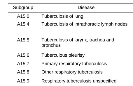
experiment was to use different algorithms to train classifiers to suggest possible diagnoses for the medical records that were not even tagged with its associated diseases. Furthermore, secondary objectives were to compare different algorithms and methods as well as different training parameters and feature sets over collected data. Diagnoses are registered based on the International Classification of Diseases (ICD), which is the standard diagnostic tool for epidemiology, health management and clinical purposes used to hierarchically classify diseases and other health problems recorded on many types of health and vital records including death certificates and health records. Tenth ICD revision (ICD-10) was endorsed by the Forty-third World Health Assembly (WHO) in May 1990 and came into use in [45] World Health Organization (WHO) Member States as from 1994 [45]. Since 2002 the public health system in the city of Florianópolis (state of Santa Catarina, Brazil) has stored over 9 million medical records related to almost 800.000 patients, and almost 50% of these medical records have no ICD-10-based associated diagnosis (no identified disease). Although in the system diseases related to the diagnosis of each patient are represented by the lowest level of ICD classification (4 characters), in this experiment was used the grouping level (3 characters) to train classifiers, since the goal of this process was just to create a tool to provide suggestions as supporting the disease diagnosis process, and not realize the proper diagnosis itself. Table 1 shows an example of a disease group (A15) and the specific diseases hierarchically associated to this group.

TABLE1

DISEASES LISTED OVER THE A15*ICD-10GROUP

6

M

Data collection used in this experiment followed a research protocol signed between the researcher and the institution that provided access to medical records, ensuring information security and confidentiality. To perform this experiment, the following steps were followed:

1. Data acquisition: 2 different datasets were selected to

perform this experiment;

2. Pre-processing: words were extracted from the

content of textual medical records;

3. Feature selection: 4 different features subsets were defined for each dataset using 2 different feature selection methods;

4. Training and testing of classifiers: KNN, MLP and

SVM were trained, validated and tested over datasets;

5. Combining classifier: classifiers were combined using

parallel and cascade methods to verify which ones

Subgroup Disease

A15.0 Tuberculosis of lung

A15.4 Tuberculosis of intrathoracic lymph nodes

A15.5 Tuberculosis of larynx, trachea and bronchus

A15.6 Tuberculous pleurisy

A15.7 Primary respiratory tuberculosis A15.8 Other respiratory tuberculosis A15.9 Respiratory tuberculosis unspecified

173 would produce better results;

6. Result analysis: results were compared to verify which

combinations of classifiers or classifiers performed better in each situation.

6.1 Data Acquisition

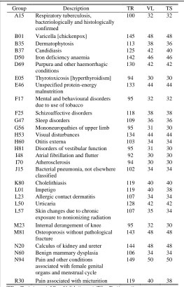
First step in this experiment was to select a dataset with medical records to perform classification, testing classifiers separately, and their parallel and serial combinations. Actually, two datasets were defined, so it was possible to evaluate the performance of classifiers in two different situations: a) smaller number of cases with greater number of classes (fewer records per class); b) largest number of cases with fewer classes (more records per class). In each dataset, records were separated into 3 groups – a training group with around 60% of the records, and validation and testing groups with 20% of the records in each one. Table 2 shows the number of records and classes per dataset. Records in dataset 1 and 2 are tagged with the disease group. Dataset 1 has 29 different classes of diseases and dataset 2 has only 15 classes. Disease groups in each dataset were selected by the similarity in the number of records per group. Tables 3 and 4 show the classes in each dataset and the number of records in each class used for training, validation and testing.

TABLE 2

Number of Classes and Records per Dataset

TABLE 3

Number of Records per Disease Group in Dataset 2

6.2 Pre-processing

Words extracted from the textual content of medical records were cleaned, and a selection of words that wouldn’t be used

was made. Cleaning process consisted of:

1. Words were extracted from medical records and converted to uppercase;

2. Words which content had digits (0-9) or just one character were not considered;

3. Plural words were converted to their singular forms; 4. Special characters (in Portuguese) were converted to

single letters (for example, "Ç" to "C" and "Á" to "A").

6.3 Feature Selection

The features used in this experiment are the words contained in the medical records. Each feature represents a word that takes the value 0 (absence) or 1 (presence) depending on whether this word appears or not in each text. Two different methods were used in feature selection, creating 4 subsets in each dataset:

1. Word frequency (WORD COUNT): total number of

times each word appears in the training dataset, considering all medical records;

2. Standard deviation (STDDEV): considering the

number of times each word appears in each class.

TABLE4

NUMBER OF RECORDS PER DISEASE GROUP IN DATASET 1

Dataset 1 Dataset 2

Number of classes 29 15

Training records 3355 9471

Validating records 1105 3158

Testing records 1092 3142

Total of records 5552 15771

Group Description TR VL TS

E10 Insulin-dependent diabetes mellitus 622 206 206

E11 Non-insulin-dependent diabetes mellitus

889 296 296

E66 Obesity 689 230 228

E78 Disorders of lipoprotein metabolism and other lipidaemias

563 188 188

F14 Mental and behavioural disorders due to use of cocaine

527 174 174

F33 Recurrent depressive disorder 506 168 168

G40 Epilepsy 497 166 166

J03 Acute tonsillitis 737 246 244

N30 Cystitis 490 162 162

N95 Menopausal and other perimenopausal disorders

665 220 220

R05 Cough 743 248 246

R07 Pain in throat and chest 645 214 214 R50 Fever of other and unknown origin 649 216 216

R51 Headache 746 248 248

R52 Pain, not elsewhere classified 503 166 166

(TR = Training set; VL = Validating set; TS = Testing set)

Group Description TR VL TS A15 Respiratory tuberculosis,

bacteriologically and histologically confirmed

100 32 32

B01 Varicella [chickenpox] 145 48 48 B35 Dermatophytosis 113 38 36 B37 Candidiasis 125 42 40 D50 Iron deficiency anaemia 142 46 46 D69 Purpura and other haemorrhagic

conditions

130 42 42

E05 Thyrotoxicosis [hyperthyroidism] 94 30 30 E46 Unspecified protein-energy

malnutrition

133 44 44

F17 Mental and behavioural disorders due to use of tobacco

95 32 32

F25 Schizoaffective disorders 118 38 38 G47 Sleep disorders 109 36 36 G56 Mononeuropathies of upper limb 95 31 30 H53 Visual disturbances 134 44 44 H60 Otitis externa 103 34 34 H81 Disorders of vestibular function 95 31 30 I48 Atrial fibrillation and flutter 92 30 30 I70 Atherosclerosis 94 30 30 J15 Bacterial pneumonia, not elsewhere

classified

102 34 34

K80 Cholelithiasis 119 40 40 L01 Impetigo 119 40 38 L23 Allergic contact dermatitis 107 34 34 L50 Urticaria 128 42 42 L57 Skin changes due to chronic

exposure to nonionizing radiation

107 35 34

M23 Internal derangement of knee 95 32 30 M81 Osteoporosis without pathological

fracture

143 48 48

N20 Calculus of kidney and ureter 144 48 48 N60 Benign mammary dysplasia 106 34 34 N94 Pain and other conditions

associated with female genital organs and menstrual cycle

149 50 50

R30 Pain associated with micturition 119 40 38

Considering the COUNT and STDDEV criteria, each dataset was applied to the classifiers considering different feature subsets: a) “W” subsets represent a feature subset where words appears more than an specific number of times (i.e., W-100 subset considers only words that appears more than W-100 times (in more than 100 medical records) in the training dataset); b) “D” subsets represent a feature subset where STDDEV of words in classes is greater than a parameter (i.e., D-10 considers only words that have STDDEV greater than 10). Table 5 shows the number of features selected in each feature subset. These different methods were used to compare classifiers´ accuracy with greater versus smaller number of features (for example, W-100 versus W-200), and also to compare results between "W" and "D" subsets (for example, W-300 versus D-40).

TABLE5

NUMBER OF SELECTED WORDS AS CLASSIFICATION FEATURES PER DATASET AND FEATURE SUBSET.

6.4 Training and Testing of Classifiers

Classifiers were trained using TR (training) and VL (validation) subsets of each dataset and tested with TS (testing) subset – except KNN which was directly tested with TS subset, since this algorithm does not have a specific validating phase. Given the nature of these classifiers that provides probabilistic answers, TOP-1 and TOP-3 accuracies were evaluated on each classifier. TOP-1 tries to find the right answer with the class that has the greater score for each tested case. TOP-3 tries to figure out the right class with the greatest three scores for each tested case. Table 6 shows the accuracies of each classifier tested with TOP-1 and TOP-3 in each dataset and feature subsets.

TABLE 6

Accuracy (%) Obtained for each Dataset After Testing each Classifier Separately.

6.5 Combining Classifiers

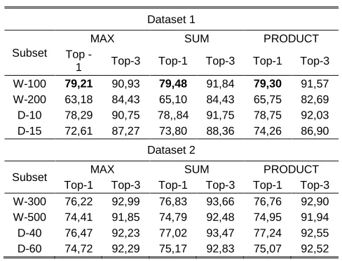
With the objective of checking whether a parallel combination of classifiers would lead them to an accuracy improvement, 3 different parallel combinations were performed (SUM, AVG and PRODUCT). Table 7 shows the obtained accuracy in each combination – results that are better than all individual classifiers are marked in bold.

TABLE 7

Accuracy (%) Obtained Combining Classifiers with Parallel Methods.

The cascade combination of classifiers was another evaluated approach. It was necessary to provide two sets of parameters: the first set refers to the order in which the classifiers would be executed; the second one refers to the acceptable probabilities concerning to the response of each classifier for each possible class. To illustrate the complexity of the problem, considering dataset 2, it would be necessary 3 parameters to indicate the order in which the classifiers would be executed sequentially (KNN, MLP and SVM) and 3 more sets of 15 parameters relating the probabilities of each class for each of the classifiers, totaling 48 parameters. To solve the problem of finding these parameter sets for each data subset, an evolutionary algorithm search was chosen, the Differential Evolution Algorithm - DE. However, due to the complexity and computational cost to process all subsets of variations that were being considered, the DE algorithm was run with a maximum of 20 generations and 20 individuals in each population. Even so, it was possible to observe that some cascading combinations achieved better results than those parallel combinations and also the best classifiers performed separately.

TABLE 8

Accuracy (%) Obtained Combining Classifiers with a Cascading Method

Feature subset Number of words (features)

D

a

ta

s

e

t

1

W-100 861

W-200 397

D-10 444

D-15 254

D

a

ta

s

e

t

2

W-300 815

W-500 482

D-40 504

D-60 315

Dataset 1

Subset

KNN MLP SVM

Top

-1 Top-3 Top-1 Top-3 Top-1 Top-3 W-100 55.31 75.55 78.02 89.38 78.66 92.58 W-200 45.60 66.12 62.00 78.02 66.67 86.63 D-10 55.59 76.83 77.75 90.38 79.49 92.12 D-15 49.18 71.34 71.89 85.35 75.18 89.38

Dataset 2

Subset KNN MLP SVM

Top-1 Top-3 Top-1 Top-3 Top-1 Top-3 W-300 59.36 83.58 74.12 89.97 77.66 94.65 W-500 55.73 82.62 71.64 88.03 76.58 93.95 D-40 60.66 85.26 73.52 88.73 77.66 94.59 D-60 61.11 84.15 70.88 88.35 77.05 94.08

Dataset 1

Subset

MAX SUM PRODUCT

Top

-1 Top-3 Top-1 Top-3 Top-1 Top-3 W-100 79,21 90,93 79,48 91,84 79,30 91,57 W-200 63,18 84,43 65,10 84,43 65,75 82,69 D-10 78,29 90,75 78,,84 91,75 78,75 92,03 D-15 72,61 87,27 73,80 88,36 74,26 86,90

Dataset 2

Subset MAX SUM PRODUCT

Top-1 Top-3 Top-1 Top-3 Top-1 Top-3 W-300 76,22 92,99 76,83 93,66 76,76 92,90 W-500 74,41 91,85 74,79 92,48 74,95 91,94 D-40 76,47 92,23 77,02 93,47 77,24 92,55 D-60 74,72 92,29 75,17 92,83 75,07 92,52

Dataset 1 Dataset 2

175 Table 8 shows the obtained accuracy of cascading

combination with the best set of parameter found by DE algorithm – results that are better than all parallel combinations are marked in bold, and results that are better than all individual classifiers are with gray background.

7

R

Considering all the results obtained during this experiment, some analyzes can be highlighted:

1. Best classifier: considering the datasets used in this experiment, SVM is the classifier with the best obtained accuracy for all tested subsets, even considering TOP-1 and TOP-3 accuracy;

2. Best feature set (greater or smaller): comparing

results of similar subsets with different number of features (for example, D-10 versus D-15, or W-300 versus W-500): a) for individual classifiers, almost all subsets with greater number of features have better accuracy then that ones with less features, except in the case of D-60 that has better accuracy than D-40 in KNN TOP-1; b) in the parallel combination of classifiers, almost all subsets with greater number of features have better accuracy then that ones with less features, except in the case of D-60 that has better accuracy than D-40 in MAX TOP-3; c) when combining classifiers with cascading method, all subsets with greater number of features have better accuracy then that ones with less features;

3. Best feature selection method: comparing results of

subsets defined with different feature selection method (for example, W-100 versus 10, or W-500 versus D-60): a) for individual classifiers, almost all subsets created with STDDEV feature have better accuracy then that ones with created with WORD-COUNT features, except in the case of W-100 that has better accuracy than D-10 in MLP TOP-1 and SVM TOP-3; b) considering the parallel combination of classifiers, W-100 has better accuracy than D-10 for almost all subsets, except in PRODUCT TOP-3, D-15 has better accuracy than W-200 for all subsets, and in dataset 2, "D" subsets have better accuracy then "W" subsets, except in MAX TOP-3 and W-300 versus D-40 in SUM TOP-3; c) when combining classifiers with cascading method, D-15 and D-60 are better than 200 and W-500 respectively; W-100 is better than D-10, and D-40 is subtly better than W-300.

4. Combining classifiers (parallel mode): in parallel

combination of classifiers only in W-100 subset in TOP-1 evaluation was possible to get better accuracy then classifiers running separately;

5. Combining classifiers (cascading mode): even using

a small population size and low number of maximum generations to find cascading parameters using DE algorithm, was possible to get some results that are better than individual classifiers and also better than combining classifiers in parallel mode.

To demonstrate some differences between individual classifiers and also between combining classifiers with different methods, some confusion matrixes and ROC analyses are presented below.

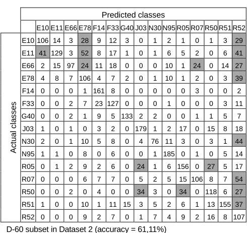
7.1 Confusion Matrixes

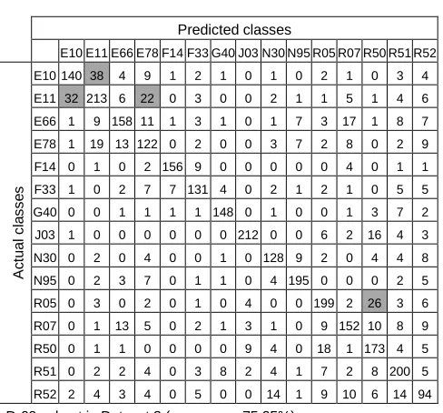
A confusion matrix is a table layout that allows visualization of the performance of a typically supervised learning algorithm, in which each column represents the instances in a predicted class, and each row represents the instances in an actual class [37]. Tables 9, 10 and 11 show the confusion matrixes for individual classifiers running over the D-60 testing record subset in dataset 2. Cells with more than 20 unmatched cases are with gray background. It´s possible to observe that common classifiers mistakes are classifying classes E11 as E10, E11 as E78 and R05 as R50.

TABLE 9

Confusion Matrix of KNN Classifier

TABLE 10

Confusion Matrix of MLP Classifier Predicted classes

E10 E11 E66 E78 F14 F33 G40 J03 N30 N95 R05 R07 R50 R51 R52

A

c

tu

a

l

c

la

s

s

e

s

E10 106 14 3 28 9 12 3 0 1 2 1 0 1 3 29 E11 41 129 3 52 8 17 1 0 1 6 5 2 0 6 41 E66 2 15 97 24 11 18 0 0 0 10 1 24 0 14 27 E78 4 8 7 106 4 7 2 0 1 10 1 2 0 3 39 F14 0 0 0 1 161 8 0 0 0 0 0 3 0 0 2 F33 0 0 2 7 23 127 0 0 0 1 0 0 0 3 11 G40 0 0 2 1 9 5 133 2 2 0 0 1 1 5 7

J03 1 0 1 0 3 2 0 179 1 2 17 0 15 8 18 N30 2 0 1 10 5 8 0 4 76 11 3 0 3 1 44 N95 1 1 0 8 0 6 0 0 1 185 0 1 0 5 14 R05 0 1 2 9 2 6 0 24 1 6 156 0 27 5 17 R07 0 0 0 6 7 7 0 5 2 5 15 106 8 7 54 R50 0 0 2 0 4 0 0 34 3 0 34 0 118 6 27 R51 1 0 0 10 1 11 15 3 5 2 6 1 13 155 37 R52 0 0 0 9 2 7 0 1 7 4 9 2 16 8 107 D-60 subset in Dataset 2 (accuracy = 61,11%)

Predicted classes

E10 E11 E66 E78 F14 F33 G40 J03 N30 N95 R05 R07 R50 R51 R52

A

ctu

a

l

class

e

s

TABLE11

CONFUSION MATRIX OF SVMCLASSIFIER

7.2 ROC Analysis

ROC analysis offers a flexible and robust framework for evaluating classifier performance with varying class distributions or misclassification costs [12], [13], [32]. A ROC plane has axes ranging from 0 to 1 and labeled false positive rate and true positive rate, and can be used to evaluate a classifier or compare different classifiers over the same database [30]. Figure 2 shows the ROC curves, comparing every separately classifier with the cascade combination of classifiers. It´s possible to identify that, even SVM has the best accuracy for the testing subset data, there are operating points which MLP and cascading combination work better.

(KNN=green; MLP=red; SVM=blue; Cascading=yellow)

Fig. 2: ROC Analysis

8

C

Based on Table 6 we observe SVM classifier achieved better accuracy in all tested subset. With this previous result, the challenge in the experiment was to combine classifiers to obtain better results than all classifiers separately. For some parallel combinations, it was possible to reach better accuracy, but in most cases this approach failed, most because SVM

accuracy is very high. When combining classifiers with a cascade approach, it was possible to identify that using an evolutionary algorithm to find the execution priority and minimal accuracy per class to consider to each classifier is a good alternative to get better accuracies in the results. Differential evolution showed itself as a good search algorithm alternative. As future work we suggest to run DE algorithm with more generations and larger populations. In this experiment we used a feature set that represents the presence or absence of each word in the textual content of medical records. This approach has a lack, when considering isolated words and not the relations between them, neither the concepts generated by this relations – for example, if words “smoke” and “don´t” appear in a text, we don’t know exactly whether it refers to a person that smoke or does not. As future work we suggest use ontologies to create concept-based feature sets instead of word-based ones.

R

[1] D.W. Aha, D. Kibler, and M.K. Albert, “Instance-based Learning Algorithms”, Machine Learning, 6:37–66, 1991.

[2] C. Bishop, “Neural Networks for Pattern Recognition”, Clarendon, Oxford, 1995.

[3] D. Bizios, A. Heij, and B. Bengtsson, “Integration and Fusion of Standard Automated Perimetry and Optical Coherence Tomography Data for Improved Automated Glaucoma Diagnostics”, BMC Ophthalmology, 11:20, 2011.

[4] O. Bousquet, O. Chapelle, and V. Vapnik, “Choosing Multiple Parameters for Support Vector Machines”, Machine Learning, 46, 131–159, 2002.

[5] A. Bulashevska and R. Eils, “Predicting Protein Subcellular Locations Using Hierarchical Ensemble of Bayesian Classifiers Based on Markov Chains”, BMC Bioinformatics, 7:298, 2006

[6] B.B. Chaudhuri and U. Bhattacharya, “Efficient Training and Improved Performance of Multilayer Perceptron in Pattern Classification”, Neurocomputing, 34:11–27, 2000.

[7] P. Corbett and A. Copestake, “Cascaded Classifiers for Confidence-based Chemical Named Entity Recognition”, Natural Language Processing in Biomedicine (BioNLP) ACL Workshop. BMC Bioinformatics, 9(Suppl 11):S4, 2008.

[8] T. Cover and P. Hart, “Nearest Nieghbor Pattern Classification”, IEEE Transaction on Information Theory, IT-13:21-27, 1967.

[9] N. Cristianini and J. Shawe-Taylor, “An Introduction to Support Vector Machines”. Cambridge University Press, 2000.

[10]S. Doan, N. Collier, H. Xu, P.H. Duy, and T.M. Phuong, “Recognition of Medication Information From Discharge Summaries Using Ensembles of Classifiers”, BMC Medical Informatics and Decision Making, 12:36, 2012 Predicted classes

E10 E11 E66 E78 F14 F33 G40 J03 N30 N95 R05 R07 R50 R51 R52

A

c

tu

a

l

c

la

s

s

e

s

177 [11]R.O. Duda, P.E. Hart, and D.G. Stork, “Pattern

Classification”, 2nd ed., John Wiley & Sons, 2000.

[12]T. Fawcett, “ROC Graphs: Notes and Practical Considerations for Researchers”, HPL-2003-4. Tech rep., HP Laboratories, 2003.

[13]P.A. Flach and S. Wu, “Repairing Concavities in ROC Curves”, In Proceedings of the 19th international joint conference on artificial intelligence”, IJCAI’05. pp. 702– 707, Edinburgh, Scotland, 2005.

[14]J. Gama and P. Brazdil, “Cascade Generalization”, Machine Learning, 41, 315–343, 2000.

[15]M.W. Gardner and S.R. Dorling, “Artificial Neural Networks (The Multilayer Perceptron): a Review of Applications in the Atmospheric Sciences”, Atmos Environ, 32:2627–2636, 1998.

[16]M. Ge, R. Du, G. Zhang, and Y. Xu, “Fault Diagnosis Using Support Vector Machine with an Application in Sheet Metal Stamping Operations”, Mechanical System and Signal Processing 12 (1) 143-159, 2004.

[17]S.R. Halgrim, F. Xia, I. Solti, E. Cadag, and O. Uzuner, “A Cascade of Classifiers for Extracting Medication Information from Discharge Summaries”, Journal of Biomedical Semantics, 2(Suppl 3):S2, 2011.

[18]S. Haykin, “Neural Networks: a Comprehensive Foundation”, Prentice Hall, 1999.

[19]S. Haykin, “Neural Networks: a Comprehensive Foundation”, 2nd ed., Prentice Hall, 2001.

[20]A.K. Jain, R.P.W. Duin, and J. Mao, “Statistical Pattern Recognition: A Review”, IEEE Transactions on Pattern Analysis and Machine Intelligence, vol. 22, n. 1, January, 2000.

[21]S. Luke, “Essentials of Metaheuristics”, Department of Computer Science, George Mason University, Online Version 1.1, January, 2011.

[22]D. Karaboga and S. Okdem, “A Simple and Global Optimization Algorithm for Engineering Problems: Differential Evolution Algorithm”, Turk J Elec Engin, 1, vol.12, 2004.

[23]A. Koussounadis, O.C. Redfern, and D.T. Jones, “Improving Classification in Protein Structure Databases Using Text Mining”, MC Bioinformatics, 10:129, 2009.

[24]M. Kukreja, S.A. Johnston, and P. Stafford, “Comparative Study of Classification Algorithms for Immunosignaturing Data”, BMC Bioinformatics, 13:139, 2012.

[25]Z. Mahmoudi, S. Rahati, M.M. Ghasemi, V. Asadpour, H. Tayarani, and M. Rajati, “Classification of Voice Disorder in Children with Cochlear Implantation and Hearing Aid Using Multiple Classifier Fusion”, BioMedical Engineering OnLine, 10:3, 2011.

[26]I. Melvin, J. Weston, C.S. Leslie, and W.S. Noble, “Combining Classifiers for Improved Classification of Proteins from Sequence or Structure”, BMC Bioinformatics, 9:389, 2008.

[27]G.P. Nam, T. Luong, H.H. Nam, K.R. Park, and S.J. Park, “Intelligent Query by Humming System Based on Score Level Fusion of Multiple Classifiers”, EURASIP Journal on Advances in Signal Processing, 21, 2011.

[28]A. Narayanan; E.C. Keedwell, and B. Olsson, “Artificial Intelligence Techniques for Bioinformatics”, Appl Bioinformatics, 1(4):191-222, 2002.

[29]G. Niu, S. Lee, B. Yang, and S. Lee, “Decision Fusion System for Fault Diagnosis of Elevator Traction Machine”, Journal of Mechanical Science and Technology 22 85-95, 2008.

[30]T. Pietraszek, “On the Use of ROC Analysis for the Optimization of Abstaining Classifiers”, Mach Learn 68: 137–169. Springer Science Business Media, LLC 2007.

[31]M. Pirooznia, J.Y. Yang, Q.U. Yang, and Y. Deng, “A Comparative Study of Different Machine Learning Methods on Microarray Gene Expression Data”, BMC Genomics, 9(Suppl 1):S13, 2008.

[32]F. Provost and T. Fawcett, “Robust Classification Systems for Imprecise Environments”, Machine Learning, 42(3), 203–231, 2001.

[33]Y. Qian, X. Li, Y. Jiang, and Y. Wen, “An Expert System for Real-time Fault Diagnosis of Complex Chemical Processes”, Expert Systems with Applications 24 (4) 425-432, 2003.

[34]S.B. Rice, G. Nenadic, and B.J. Stapley, “Mining Protein Function from Text Using Term-based Support Vector Machines”. BMC Bioinformatics, 6(Suppl 1):S22, 2005.

[35]B. Samanta and K.R. Al-Balushi, “Artificial Neural Network Based Fault Diagnostics of Rolling Element Bearings Using Time-domain Features”, Mechanical System and Signal Processing 17 (2) 317-328, 2003.

[36]A. Slowik, “Application of an Adaptive Differential Evolution Algorithm With Multiple Trial Vectors to Artificial Neural Network Training”, IEEE Transactions on Industrial Electronics, 8, vol. 58, pp. 3160-3167, August, 2011.

[37]S.V. Stehman, "Selecting and Interpreting Measures of Thematic Classification Accuracy", Remote Sensing of Environment 62 (1): 77–89, 1997.

[38]R. Storn and K. Price, “Differential Evolution - A Simple and Efficient Heuristic for Global Optimization over Continuous Spaces”, Journal of Global Optimization, Vol. 11, pp 341-359, Netherlands, 1997.

Computation, vol.3, pp. 22:3, 1999.

[40]M. Tipping, “Sparse Bayesian Learning and the Relevance Vector Machine”, Journal of Machine Learning Research 1 211-244, 2001.

[41]G. Valenti, M. Lelli, and D. Cucina, “A Comparative Study of Models for the Incident Duration Prediction”, Eur. Transp. Res. Rev. 2:103–111, 2010.

[42]V. Vapnik, “An Overview of Statistical Learning Theory”, IEEE Trans Neural Netw 10(5):988–999, 1999.

[43]M. Wakil, “Introducing Text Mining”, in 9th Scientific Conference for Information Systems and Information Technology, February, 2002.

[44]K. Weinberger, J. Blitzer, and L. Saul,“Distance Metric Learning for Large Margin Nearest Neighbor Classification”, J Mach Learn Res, 10:207–244, 2009.

[45]World Health Organization, “International Statistical Classification of Diseases and Related Health Problems, Tenth Revision, 1992.