Performance analysis model for big data applications in cloud computing

(1)

R E S E A R C H

Open Access

Performance analysis model for big data

applications in cloud computing

Luis Eduardo Bautista Villalpando

1,2*

, Alain April

2

and Alain Abran

2

Abstract

The foundation of Cloud Computing is sharing computing resources dynamically allocated and released per demand with minimal management effort. Most of the time, computing resources such as processors, memory and storage are allocated through commodity hardware virtualization, which distinguish cloud computing from others technologies. One of the objectives of this technology is processing and storing very large amounts of data, which are also referred to as Big Data. Sometimes, anomalies and defects found in the Cloud platforms affect the

performance of Big Data Applications resulting in degradation of the Cloud performance. One of the challenges in Big Data is how to analyze the performance of Big Data Applications in order to determine the main factors that affect the quality of them. The performance analysis results are very important because they help to detect the source of the degradation of the applications as well as Cloud. Furthermore, such results can be used in future resource planning stages, at the time of design of Service Level Agreements or simply to improve the applications. This paper proposes a performance analysis model for Big Data Applications, which integrates software quality concepts from ISO 25010. The main goal of this work is to fill the gap that exists between quantitative (numerical) representation of quality concepts of software engineering and the measurement of performance of Big Data Applications. For this, it is proposed the use of statistical methods to establish relationships between extracted performance measures from Big Data Applications, Cloud Computing platforms and the software engineering quality concepts.

Keywords:Cloud computing; Big data; Analysis; Performance; Relief algorithm; Taguchi method; ISO 25010; Maintenance; Hadoop MapReduce

Introduction

According to ISO subcommittee 38, the CC study group, Cloud Computing (CC) is a paradigm for enabling ubi-quitous, convenient, on-demand network access to a shared pool of configurable cloud resources accessed through services which can be rapidly provisioned and released with minimal management effort or service pro-vider interaction [1].

One of the challenges in CC is how to process and store large amounts of data (also known as Big Data ? BD) in an efficient and reliable way. ISO subcommittee 32, Next Generation Analytics and Big Data study group, refers Big Data as the transition from structured data

and traditional analytics to analysis of complex informa-tion of many types. Moreover, the group meninforma-tions that Big Data exploits cloud resources to manage large data volume extracted from multiple sources [2]. In December 2012, the International Data Corporation (IDC) stated that, by the end of 2012, the total data generated was 2.8 Zettabytes (ZB) (2.8 trillion Gigabytes). Furthermore, the IDC predicts that the total data generated by 2020 will be 40 ZB. This is roughly equivalent to 5.2 terabytes (TB) of data generated by every human being alive in that year [3]. Big Data Applications (BDA) are a way to process a part of such large amounts of data by means of plat-forms, tools and mechanisms for parallel and distributed processing. ISO subcommittee 32 mentions that BD An-alytics has become a major driving application for data warehousing, with the use of MapReduce outside and in-side of database management systems, and the use of self-service data marts [2]. MapReduce is one of the * Correspondence:[email protected]

1

Department of Electronic Systems, Autonomous University of Aguascalientes, Av. Universidad 940, Ciudad Universitaria, Aguascalientes, Mexico

2_{Department of Software Engineering and Information Technology ETS,} University of Quebec, 1100 Notre-Dame St., Montreal, Canada

(2)

programming models used to develop BDA, which was developed by Google for processing and generating large datasets.

Sometimes, anomalies and defects found in platforms of Cloud Computing Systems (CCS) affect the perform-ance of BDA resulting in degradation of the whole sys-tem. Performance analysis models (PAM) for BDA in CC, should propose a means to identify and quantify

?normal application behaviour? , which can serve as a baseline for detecting and predicting possible anomalies in the software (i.e. applications in a Big Data platforms) that may impact BDA itself. To be able to design such PAM for BDA, methods are needed to collect the neces-sary base measures specific to performance, and a per-formance framework must be used to determine the relationships that exist among these measures.

One of the challenges in designing PAM for BDA is how to determine what type of relationship exists be-tween the various base measures and the performance quality concepts defined in international standards such as ISO 25010 [4]. For example, what is the extent of the relationship between the amounts of physical memory used by a BDA and the performance quality concepts of software engineering such as resource utilization or cap-acity? Thus, this work proposes the use of statistical methods to determine how closely performance parame-ters (base measures) are related with performance con-cepts of software engineering.

This paper is structured as follows. Related work and background sections present the concepts related to the performance measurement of BDA and introduces the MapReduce programming model. In addition, back-ground section presents the Performance Measurement Framework for Cloud Computing (PMFCC), which de-scribes the key performance concepts and sub concepts that the best represent the performance of CCS. Analysis model section, presents the method for examining the relationships among the performance concepts identified in the PMFCC. An experimental methodology based on the Taguchi method of experimental design, is used and offers a means for improving the quality of product per-formance. Experiment section presents the results of an experiment, which analyzes the relationship between the performance factors of BDA, Cloud Computing Plat-forms (CCP) and the performance concepts identified in the PMFCC. Finally, conclusion section presents a syn-thesis of the results of this research and suggests future work.

Related work

Researchers have analyzed the performance of BDA from various viewpoints. For example, Alexandru [5] an-alyzes the performance of Cloud Computing Services for Many-Task Computing (MTC) system. According to

Alexandru, scientific workloads often require High-Performance Computing capabilities, in which scientific computing community has started to focus on MTC, this means high performance execution of loosely coupled applications comprising many tasks. By means of this approach it is possible to demand systems to op-erate at high utilizations, like to current production grids. Alexandru analyzes the performance based on the premise if current clouds can execute MTC-based scientific workload with similar performance and at lower cost that the current scientific processing sys-tems. For this, the author focuses on Infrastructures as a Service (IaaS), this means providers on public clouds that are not restricted within an enterprise. In this re-search, Alexandru selected four public clouds providers; Amazon EC2, GoGrid, ElasticHosts and Mosso in which it is performed a traditional system benchmark-ing in order to provide a first order estimate of the system performance. Alexandru mainly uses metrics related to disk, memory, network and cpu to deter-mine the performance through the analysis of MTC workloads which comprise tens of thousands to hun-dreds of thousands of tasks. The main finding in this research is that the compute performance of the tested clouds is low compared to traditional systems of high performance computing. In addition, Alexandru found that while current cloud computing services are insuffi-cient for sinsuffi-cientific computing at large, they are a good solution for scientists who need resources instantly and temporarily.

(3)

to cost (in dollars, energy or other value propositions). The results show a strong correlation between the per-centage of time an application spends communicating, and its overall performance on EC2. The more commu-nication there is, the worse the performance becomes. Jackson also concludes that the communication pattern of an application can have a significant impact on performance.

Other researchers focus their work on the performance analysis of MapReduce applications. For example, Jin [8] proposes a stochastic model to predict the performance of MapReduce applications under failures. His work is used to quantify the robustness of MapReduce applications under different system parameters, such as the number of processes, the mean time between failures (MTBF) of each process, failure recovery cost, etc. Authors like Jiang [9], performs a depth study of factors that affect the perform-ance of MapReduce applications. In particular, he identi-fies five factors that affect the performance of MapReduce applications: I/O mode, indexing, data parsing, grouping schemes and block level scheduling. Moreover, Jiang con-cludes that carefully tuning each factor, it is possible to eliminate the negative impact of these factors and improve the performance of MapReduce applications. Other au-thors like Guo [10] and Cheng [11] focus their works on improving the performance of MapReduce applications. Gou explodes the freedom to control concurrency in MapReduce in order to improve resource utilization. For this, he proposes ? resource stealing? which dynamically expands and shrinks the resource usage of running tasks by means of the benefit aware speculative execution (BASE). BASE improves the mechanisms of fault-tolerance managed by speculatively launching duplicate tasks for tasks deemed to be stragglers. Furthermore, Cheng [11] focuses his work on improving the perform-ance of MapReduce applications through a strategy called maximum cost performance (MCP). MCP im-proves the effectiveness of speculative execution by means of accurately and promptly identifying stragglers. For this he provides the following methods: 1) Use both the progress rate and the process bandwidth within a phase to select slow tasks, 2) Use exponentially weighted moving average (EWMA) to predict process speed and calculate a task?s remaining time and 3) De-termine which task to backup based on the load of a cluster using a cost-benefit model.

Although these works present interesting methods for the performance analysis of CCS and improving of BD applications (MapReduce), their approach is from an infrastructure standpoint and does not consider the performance from a software engineering perspective. This work focuses on the performance analysis of BDA developed by means of the Hadoop MapReduce model, integrating software quality concepts from ISO 25010.

Background

Hadoop MapReduce

Hadoop is the Apache Software Foundation?s top level project, and encompasses the various Hadoop sub pro-jects. The Hadoop project provides and supports the de-velopment of open source software that supplies a framework for the development of highly scalable dis-tributed computing applications designed to handle pro-cessing details, leaving developers free to focus on application logic [12]. Hadoop is divided into several sub projects that fall under the umbrella of infrastructures for distributed computing. One of these sub projects is MapReduce, which is a programming model with an as-sociated implementation, both developed by Google for processing and generating large datasets.

According to Dean [13], programs written in this func-tional style are automatically parallelized and executed on a large cluster of commodity machines. Authors like Lin [14] point out that today, the issue of tackling large amounts of data is addressed by a divide-and-conquer approach, the basic idea being to partition a large prob-lem into smaller sub probprob-lems. Those sub probprob-lems can be handled in parallel by different workers; for example, threads in a processor core, cores in a multi-core proces-sor, multiple processors in a machine, or many machines in a cluster. In this way, the intermediate results of each individual worker are then combined to yield the final output.

The Hadoop MapReduce model results are obtained in two main stages: 1) the Map stage, and 2) the Reduce stage. In the Map stage, also called the mapping phase, data elements from a list of such elements are inputted, one at time, to a function called Mapper, which trans-forms each element individually into an output data element. Figure 1 presents the components of the Map stage process.

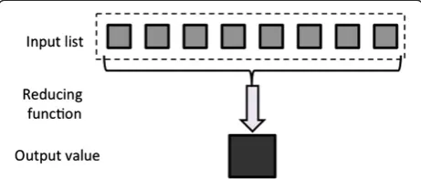
The Reduce stage (also called the reducing phase) ag-gregates values. In this stage, a reducer function receives input values iteratively from an input list. This function combines these values, returning a single output value. The Reduce stage is often used to produce ? summary? data, turning a large volume of data into a smaller sum-mary of itself. Figure 2 presents the components of the Reduce stage.

(4)

According to Yahoo! [15], when a mapping phase be-gins, any mapper (node) can process any input file or part of an input file. In this way, each mapper loads a set of local files to be able to process them. When a map-ping phase has been completed, an intermediate pair of values (consisting of a key and a value) must be ex-changed between machines, so that all values with the same key are sent to a single reducer. Like Map tasks, Reduce tasks are spread across the same nodes in the cluster and do not exchange information with one an-other, nor are they aware of one another?s existence. Thus, all data transfer is handled by the Hadoop MapRe-duce platform itself, guided implicitly by the various keys associated with the values.

Performance measurement framework for cloud computing

The Performance Measurement Framework for Cloud Computing (PMFCC) [16] is based on the scheme for performance analysis shown in Figure 3. This scheme es-tablishes a set of performance criteria (or characteristics) to help to carry out the process of analysis of system performance. In this scheme, the system performance is typically analyzed using three sub concepts, if it is per-forming a service correctly: 1) responsiveness, 2) prod-uctivity, and 3) utilization, and proposes a measurement process for each. There are several possible outcomes

for each service request made to a system, which can be classified into three categories. The system may: 1) per-form the service correctly, 2) perper-form the service incor-rectly, or 3) refuse to perform the service altogether. Moreover, the scheme defines three sub concepts associ-ated with each of these possible outcomes, which affect system performance: 1) speed, 2) reliability, and 3) avail-ability. Figure 3 presents this scheme, which shows the possible outcomes of a service request to a system and the sub concepts associated with them.

Based on the above scheme, the PMFCC [16] maps the possible outcomes of a service request onto quality con-cepts extracted from the ISO 25010 standard. The ISO 25010 [4] standard defines software product and computer system quality from two distinct perspectives: 1) a quality in use model, and 2) a product quality model. The product quality model is applicable to both systems and software. According to ISO 25010, the properties of both determine the quality of the product in a particular context, based on user requirements. For example, performance efficiency and reliability can be specific concerns of users who specialize in areas of content delivery, management, or maintenance. The performance efficiency concept pro-posed in ISO 25010 has three sub concepts: 1) time behav-ior, 2) resource utilization, and 3) capacity, while the reliability concept has four sub concepts: 1) maturity, 2) availability, 3) fault tolerance, and 4) recoverability. The PMFCC selects performance efficiency and reliability as concepts for determining the performance of CCS. In addition, the PMFCC proposes the following definition of CCS performance analysis:

?The performance of a Cloud Computing system is determined by analysis of the characteristics involved in performing an efficient and reliable service that meets requirements under stated conditions and within the maximum limits of the system parameters?.

Once that the performance analysis concepts and sub concepts are mapped onto the ISO 25010 quality con-cepts, the framework presents a model of relationship (Figure 4) that presents a logical sequence in which the concepts and sub concepts appear when a performance issue arises in a CCS.

In Figure 4, system performance is determined by two main sub concepts: 1) performance efficiency, and 2) reli-ability. We have seen that when a CCS receives a service request, there are three possible outcomes (the service is performed correctly, the service is performed incorrectly, or the service cannot be performed). The outcome will de-termine the sub concepts that will be applied for perform-ance analysis. For example, suppose that the CCS performs a service correctly, but, during its execution, the service failed and was later reinstated. Although the service was Figure 2The components of the reducing phase.

(5)

ultimately performed successfully, it is clear that the system availability (part of the reliability sub concept) was compro-mised, and this affected CCS performance.

Performance analysis model for big data applications

Relationship between performance measures of BDA, CCP and software engineering quality concepts

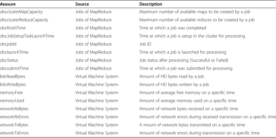
In order to determine the degree of relationship between performance measures of BDA, and performance con-cepts and sub concon-cepts defined in the PMFCC (Figure 4), first it is necessary to map performance measures from the BDA and CCP onto the performance quality con-cepts previously defined. For this, measures need to be collected by means of extracted data from MapReduce log files and system monitoring tools (see Table 1). This data is obtained from a Hadoop cluster, which is the cloud platform in which the CCS is running.

Once the performance measures are collected, they are mapped onto the performance concepts defined in the PMFCC by means of the formulae defined in the ISO 25023. ISO 25023 - Measurement of system and software

product quality, provides a set of quality measures for the characteristics of system/software products that can be used for specifying requirements, measuring and evaluat-ing the system/software product quality [17]. It is import-ant to mention that such formulae were adapted according to the different performance measures collected from the BDA and CCP in order to represent the different concepts in a coherent form. Table 2 presents the different BDA and CCP performance measures after being mapped onto the PMFCC concepts and sub concepts.

Selection of key PMFCC concepts to represent the performance of BDA

(6)

concepts) for building robust learning models by removing most irrelevant and redundant features from the data. Kantardzic establishes that feature selection algorithms typically fall into two categories: feature ranking and subset selection. Feature ranking ranks all features by a specific base measure and eliminates all features that do not achieve an adequate score while subset selec-tion, searches the set of all features for the optimal subset in which selected features are not ranked. The next subsections present two techniques of feature ranking which are used in the PAM for BDA in order to determine the most relevant performance sub con-cepts (features) that best represent the performance of BDA.

Feature selection based on comparison of means and variances

The feature selection based on comparison of means and variances is based on the distribution of values for a given feature, in which it is necessary to compute the mean value and the corresponding variance. In general, if one feature describes different classes of entities, samples of two different classes can be examined. The means of feature values are normalized by their vari-ances and then compared. If the means are far apart, interest in a feature increases: it has potential, in terms of its use in distinguishing between two classes. If the means are indistinguishable, interest wanes in that fea-ture. The mean of a feature is compared in both cases without taking into consideration relationship to other features. The next equations formalize the test, where

A and B are sets of feature values measured for two dif-ferent classes, and n1 and n2 are the corresponding

number of samples:

SE A? −B? ?

ffiffiffiffiffiffiffiffiffiffiffiffiffiffiffiffiffiffiffiffiffiffiffiffiffiffiffiffiffiffiffiffiffiffiffiffiffiffiffiffiffi

var? ?A n1 ?

var? ?B n2

s

? 1?

Test: jmean A? ? −mean B? ? j

SE A? −B? >threshold value ? 2?

In this approach to feature selection, it is assumed that a given feature is independent of others. A comparison of means is typically a natural fit to classification prob-lems. For k classes, k pair wise comparisons can be made, comparing each class with its complement. A fea-ture is retained if it is significant for any of the pair wise comparisons as shown in formula 2.

Relief algorithm

Another important technique for feature selection is the Relief algorithm. The Relief algorithm is a feature weight-based algorithm, which relies on relevance evaluation of each feature given in a training data set in which samples are labeled (classification problems). The main concept of this algorithm is to compute a ranking score for every feature indicating how well this feature separates neighboring samples. The authors of the Relief algorithm, Kira and Rendell [19], proved that ranking

Table 1 Extract of collected performance measures from the BDA and CCP

Measure Source Description

jobs:clusterMapCapacity Jobs of MapReduce Maximum number of available maps to be created by a job

jobs:clusterReduceCapacity Jobs of MapReduce Maximum number of available reduces to be created by a job

jobs:finishTime Jobs of MapReduce Time at which a job was completed

jobs:JobSetupTaskLaunchTime Jobs of MapReduce Time at which a job is setup in the cluster for processing

jobs:jobId Jobs of MapReduce Job ID

jobs:launchTime Jobs of MapReduce Time at which a job is launched for processing

jobs:Status Jobs of MapReduce Job status after processing (Successful or Failed)

jobs:submitTime Jobs of MapReduce Time at which a job was submitted for processing

disk:ReadBytes Virtual Machine System Amount of HD bytes read by a job

disk:WriteBytes Virtual Machine System Amount of HD bytes written by a job

memory:Free Virtual Machine System Amount of average free memory on a specific time

memory:Used Virtual Machine System Amount of average memory used on a specific time

network:RxBytes Virtual Machine System Amount of network bytes received on a specific time

network:RxErrors Virtual Machine System Amount of network errors during received transmission on a specific time

network:TxBytes Virtual Machine System A mount of network bytes transmitted on a specific time

(7)

score becomes large for relevant features and small for irrelevant ones.

The objective of the relief algorithm is to estimate the quality of features according to how well their values distinguish between samples close to each other. Given a training dataS, the algorithm randomly selects subset of samples size m, where m is a user defined parameter. The algorithm analyses each feature based on a selected subset of samples. For each randomly selected sampleX from a training data set, it searches for its two nearest neighbors: one from the same class, called nearest hitH, and the other one from a different class, called nearest missM.

The Relief algorithm updates the quality scoreW(Ai) for all featureAidepending on the differences on their values for samplesX,M, andHas shown in formula 3.

Wnew? ?Ai ? Wold? ?Ai −diff X A? ? i; H A? i?

2

? diff X A? ? i; M A? i? 2

m

? 3?

The process is repeated mtimes for randomly selected samples from the training data set and the scores W(Ai) are accumulated for each sample. Finally, using threshold of relevancy τ, the algorithm detects those features that are statistically relevant to the target classification, and

Table 2 BDA and CCP performance measures mapped onto PMFCC concepts and sub concepts

PMFCC concept

PMFCC sub concepts

Description Adapted formula

Performance efficiency

Time behavior

Response time Duration from a submitted BDA Job to start processing till it is launched

submitTime - launchTime

Time behavior

Turnaround time Duration from a submitted BDA Job to start processing till completion of the Job

finishTime? submitTime

Time behavior

Processing time Duration from a launched BDA Job to start processing till completion of the Job

finishTime-launchTime

Resource utilization

CPU utilization How much CPU time is used per minute to process a BDA Job (percent)

100_? cpuIdlePercent

Memory utilization How much memory is used to process a BDA Job per minute (percent)

100? memoryFreePercent

Hard disk bytes read How much bytes are read to process a BDA Job per minute Total of bytes read per minute

Hard disk bytes written

How much bytes are written to process a BDA Job per minute Total of bytes written per minute

Capacity Load map tasks capacity

How many map tasks are processed in parallel for a specific BDA Job

Total of map tasks processed in parallel for a specific BDA Job

Capacity Load reduce tasks capacity

How many reduce tasks are processed in parallel for a specific BDA Job

Total of reduce tasks processed in parallel for a specific BDA Job

Capacity Network Tx bytes How many bytes are transferred while a specific BDA Job is processed

Total of transferred bytes per minute

Capacity Network Rx bytes How many bytes are received while a specific BDA Job is processed

Total of received bytes per minute

Reliability

Maturity Task mean time between failure

How frequently does a task of a specific BDA Job fail in operation

Number of tasks failed per minute

Maturity Tx network errors How many transfer errors in the network are detected while processing a specific BDA Job

Number of Tx network errors detected per minute

Maturity Rx network errors How many reception errors in the network are detected while processing a specific BDA Job

Number of Rx network errors detected per minute

Availability Time of CC System Up

Total time that the system has been in operation Total minutes of the CC system operation

Fault tolerance

Network Tx collisions How many transfer collision in the network occurs while processing a specific BDA Job

Total of Tx network collisions per minute

Fault tolerance

Network Rx dropped How many reception bytes in the network are dropped while processing a specific BDA Job

Total of Rx network bytes are dropped per minute

Recoverability Mean recovery time What is the average time the CC system take to complete recovery from a failure

(8)

these are the features withW(Ai)≥τ. The main steps of the Relief algorithm are formalized in Algorithm 1.

Choosing a methodology to analyze relationships between performance concepts

Once that a subset of the most important features (key performance sub concepts) has been selected, the next step is to determine the degree of relationship that exist between such subset of features and the rest of perform-ance sub concepts defined by means of PMFCC. For this, the use of Taguchi?s experimental design method is proposed: it investigates how different features (perform-ance measures) are related, and to what degree. Under-standing these relationships will enable us to determine the influence each of them has in the resulting perform-ance concepts. The PMFCC shows many of the relation-ships that exist between the base measures, which have a major influence on the collection functions. However, in BDA and more specifically in the Hadoop MapReduce application experiment, there are over a hundred pos-sible performance measures (including system measures) that could contribute to the analysis of BDA performance. A selection of these performance measures has to be in-cluded in the collection functions so that the respective performance concepts can be obtained and, from there, an indication of the performance of the applications. One key design problem is to establish which performance mea-sures are interrelated and how much they contribute to each of the collection functions.

In traditional statistical methods, thirty or more obser-vations (or data points) are typically needed for each vari-able, in order to gain meaningful insights and analyze the results. In addition, only a few independent variables are necessary to carry out experiments to uncover potential relationships, and this must be performed under certain predetermined and controlled test conditions. However, this approach is not appropriate here, owing to the large number of variables involved and the considerable time and effort required. Consequently, an analysis method that is suited to our specific problem and in our study area is needed.

A possible candidate method to address this problem is Taguchi?s experimental design method, which investigates

how different variables affect the mean and variance of a process performance characteristics, and helps in deter-mining how well the process is functioning. This Taguchi method proposes a limited number of experiments, but is more efficient than a factorial design in its ability to iden-tify relationships and dependencies. The next section pre-sents the method to find out the relationships.

Taguchi method of experimental design

Taguchi?s Quality Engineering Handbook [20] describes the Taguchi method of experimental design which was developed by Dr. Genichi Taguchi, a researcher at the Electronic Control Laboratory in Japan. This method combines industrial and statistical experience, and offers a means for improving the quality of manufactured prod-ucts. It is based on a?robust design? concept, according to which a well designed product should cause no problem when used under specified conditions.

According to Cheikhi [21], Taguchi?s two phase quality strategy is the following:

Phase 1: The online phase, which focuses on the

techniques and methods used to control quality during the production of the product.

Phase 2: The offline phase, which focuses on taking

those techniques and methods into account before manufacturing the product, that is, during the design phase, the development phase, etc.

One of the most important activities in the offline phase of the strategy is parameter design. This is where the parameters are determined that makes it possible to satisfy the set quality objectives (often called the object-ive function) through the use of experimental designs under set conditions. If the product does not work properly (does not fulfill the objective function), then the design con-stants (also called parameters) need to be adjusted so that it will perform better. Cheikhi [21] explains that this activity includes five (5) steps, which are required to determine the parameters that satisfy the quality objectives:

1. Definition of the objective of the study, that is, identification of the quality characteristics to be observed in the output (results expected). 2. Identification of the study factors and their

interactions, as well as the levels at which they will be set. There are two different types of factors: 1) control factors: factors that can be easily managed or adjusted; and 2) noise factors: factors that are difficult to control or manage.

(9)

various experiments that will need to be conducted in order to verify the effect of the factors studied on the quality characteristic to be observed in the output.

4. Preparation and performance of the resulting OA experiments, including preparation of the data sheets for each OA experiment according to the combination of the levels and factors for the experiment. For each experiment, a number of trials are conducted and the quality characteristics of the output are observed.

5. Analysis and interpretation of the experimental results to determine the optimum settings for the control factors, and the influence of those factors on the quality characteristics observed in the output.

According to Taguchi?s Quality Engineering Hand-book [20] the OA organizes the parameters affecting the process and the levels at which they should vary. Taguchi?s method tests pairs of combinations, instead of having to test all possible combinations (as in a fac-torial experimental design). This approach can deter-mine which factors affect product quality the most in a minimum number of experiments.

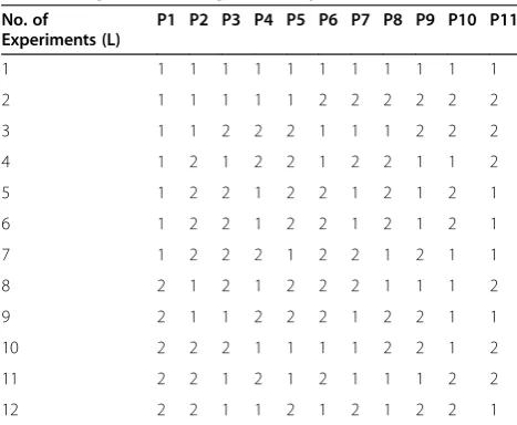
Taguchi?s OA can be created manually or they can be derived from deterministic algorithms. They are selected by the number of parameters (variables) and the number of levels (states). An OA array is represented by Ln and Pn, where Ln corresponds to the number of experiments to be conducted, and Pn corresponds to the number of parameters to be analyzed. Table 3 presents an example of Taguchi OA L12, meaning that 12 experiments are conducted to analyze 11 parameters.

An OA cell contains the factor levels (1 and 2), which determine the type of parameter values for each experiment. Once the experimental design has

been determined and the trials have been carried out, the performance characteristic measurements from each trial can be used to analyze the relative effect of the vari-ous parameters.

Taguchi?s method is based on the use of the signal-to-noise ratio (SNR). The SNR is a measurement scale that has been used in the communications industry for nearly a century for determining the extent of the relationship between quality factors in a measurement model [20]. The SNR approach involves the analysis of data for variability in which an input-to-output relationship is studied in the measurement system. Thus, to determine the effect each parameter has on the output, the SNR is calculated by the follow formula:

SNi? 10 log

y2 i

S2_i ? 4?

Where

y_i? 1 Ni

XNi

u? 1

y_i_;_u

S2_i ? 1 Ni−1

XNi

u? 1

y_i_;_u−y_i

i=Experiment number u=Trial number

Ni=Number of trials for experimenti

To minimize the performance characteristic (objective function), the following definition of the SNR should be calculated:

SNi? −10 log

XNi

u? 1

y2_u Ni

!

? 5?

To maximize the performance characteristic (objective function), the following definition of the SNR should be calculated:

SNi? −10 log 1

Ni

XNi

u? 1 1

y2 u

" #

? 6?

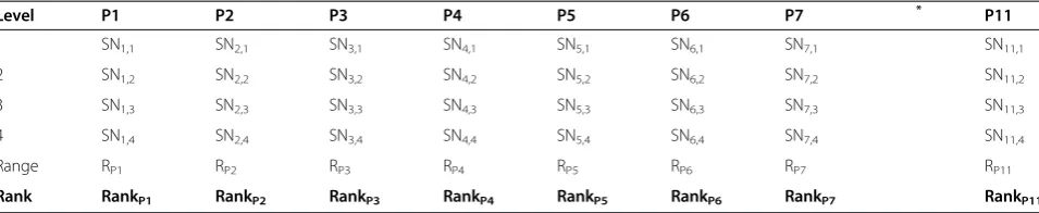
Once the SNR values have been calculated for each factor and level, they are tabulated as shown in Table 4, and then the range R (R = high SN - low SN) of the SNR for each parameter is calculated and entered on Table 4.

According to Taguchi?s method, the larger the R value for a parameter, the greater its effect on the process.

Table 3 Taguchi?s Orthogonal Array L12

No. of Experiments (L)

P1 P2 P3 P4 P5 P6 P7 P8 P9 P10 P11

1 1 1 1 1 1 1 1 1 1 1 1

2 1 1 1 1 1 2 2 2 2 2 2

3 1 1 2 2 2 1 1 1 2 2 2

4 1 2 1 2 2 1 2 2 1 1 2

5 1 2 2 1 2 2 1 2 1 2 1

6 1 2 2 1 2 2 1 2 1 2 1

7 1 2 2 2 1 2 2 1 2 1 1

8 2 1 2 1 2 2 2 1 1 1 2

9 2 1 1 2 2 2 1 2 2 1 1

10 2 2 2 1 1 1 1 2 2 1 2

11 2 2 1 2 1 2 1 1 1 2 2

(10)

Experiment

Experiment setup

The experiment was conducted on a DELL Studio Workstation XPS 9100 with Intel Core i7 12-core X980 processor at 3.3 GHz, 24 GB DDR3 RAM, Seagate 1.5 TB 7200 RPM SATA 3Gb/s disk, and 1 Gbps network connection. We used a Linux CentOS 6.4 64-bit distri-bution and Xen 4.2 as the hypervisor. This physical ma-chine hosts five virtual mama-chines (VM), each with a dual-core Intel i7 configuration, 4 GB RAM, 20 GB vir-tual storage, and a virvir-tual network interface type. In addition, each VM executes the Apache Hadoop distri-bution version 1.0.4, which includes the Hadoop Distrib-uted File System (HDFS) and MapReduce framework libraries, Apache Chukwa 0.5.0 as performance mea-sures collector and Apache HBase 0.94.1 as perform-ance measures repository. One of these VM is the

master node, which executes NameNode (HDFS) and JobTracker (MapReduce), and the rest of the VM are slave nodes running DataNodes (HDFS) and JobTrackers (MapReduce). Figure 5 presents the cluster configuration for the set of experiments.

Mapping of performance measures onto PMFCC concepts

A total of 103 MapReduce Jobs (BDA) were executed in the virtual Hadoop cluster and a set of performance measures were obtained from MapReduce Jobs logs and monitoring tools. One of the main problems that arose after the performance measures repository ingestion process was the cleanliness of data. Cleanliness calls for the quality of the data to be verified prior to performing data analysis. Among the most important data quality issues to consider during data cleaning in the model were corrupted records, inaccurate content, missing values, and

Table 4 Rank for SNR values

Level P1 P2 P3 P4 P5 P6 P7 ? * P11

1 SN1,1 SN2,1 SN3,1 SN4,1 SN5,1 SN6,1 SN7,1 ? SN11,1

Range RP1 RP2 RP3 RP4 RP5 RP6 RP7 ? RP11

Rank RankP1 RankP2 RankP3 RankP4 RankP5 RankP6 RankP7 ? RankP11

*Corresponding values for parameters P8, P9 and P10.

(11)

formatting inconsistencies, to name a few. Consequently, one of the main challenges at the preprocessing stage was how to structure data in standard formats so that they can be analyzed more efficiently. For this, a data normalization process was carried out over the data set by means of the standard score technique (see formula 7).

Xnormi?

Xi−μi

Si ?

7?

where

Xi=Featurei

μi=Average value ofXiin data set

Si=Range of featurei(MaxXi-MinXi)

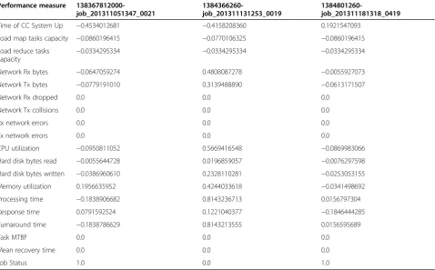
The normalization process scaled the values between the range of [-1, 1] according to the different collected performance measures which are expressed in different units and dimensions. For example the measure process-ing time is expressed in minutes while the measure mem-ory utilization is expressed in Mbytes. Table 5 presents an extract from the different collected performance measures after the process of normalization.

Note: Table 5 shows that values related to network mea-sures are equal to zero because the experiment is per-formed in a Hadoop virtual cluster. This means that real

transmission over a physical network does not exist leaving out the possibility of errors. In addition, other measures such as mean time between failure and mean recovery time are also equal to zero because during the experiment dur-ation Hadoop virtual cluster never failed.

Selection of key measures to represent the performance of BDA

One of the challenges in the design of the PAM for BDA is how to determine a set of key sub concepts which have more relevance in the performance compared to others. For this, the application of feature selection is used during the process for knowledge discovery. As previously mentioned, two techniques used for feature selection are: means and variances, and the Relief algo-rithm. The means and variances approach assumes that the given features are independent of others. In the ex-periment a total of 103 Hadoop MapReduce Jobs were executed storing their performance measures. A MapRe-duce Job may belong to one of two classes according to its status; failed or successful (0 or 1) (see Table 5).

Thus, applying means and variances technique to the data set, the feature Job Status classifies each Job records into two classes 0 and 1. First, it is necessary to compute a mean value and variance for both classes and for each fea-ture (PMFCC sub concept measure). It is important to note that test values will be compared with the highest set

Table 5 Extract of collected performance measures after process of normalization

Performance measure

138367812000-job_201311051347_0021

1384366260-job_201311131253_0019

1384801260-job_201311181318_0419

Time of CC System Up −0.4534012681 −0.4158208360 0.1921547093

Load map tasks capacity −0.0860196415 −0.0770106325 −0.0860196415

Load reduce tasks capacity

−0.0334295334 −0.0334295334 −0.0334295334

Network Rx bytes −0.0647059274 0.4808087278 −0.0055927073

Network Tx bytes −0.0779191010 0.3139488890 −0.0613171507

Network Rx dropped 0.0 0.0 0.0

Network Tx collisions 0.0 0.0 0.0

Rx network errors 0.0 0.0 0.0

Tx network errors 0.0 0.0 0.0

CPU utilization −0.0950811052 0.5669416548 −0.0869983066

Hard disk bytes read −0.0055644728 0.0196859057 −0.0076297598

Hard disk bytes written −0.0386960610 0.2328110281 −0.0253053155

Memory utilization 0.1956635952 0.4244033618 −0.0341498692

Processing time −0.1838906682 0.8143236713 0.0156797304

Response time 0.0791592524 0.1221040377 −0.1846444285

Turnaround time −0.1838786629 0.8143213555 0.0156595689

Task MTBF 0.0 0.0 0.0

Mean recovery time 0.0 0.0 0.0

(12)

of values obtained after the ranking process (0.9) because this distinguished them from the rest of results. Results are shown in Table 6.

The analysis shows that measures job processing time and job turnaroundhave the potential to be distinguish-ing features between the two classes because their means are far apart and interest in such measures in-creases, this means their test values are greater than 0.9. In addition, it is important to mention that although be-tween the second and third result (hard disk bytes writ-ten) there is a considerable difference; the latter is also selected in order to analyze its relationship with the rest of measures because it also has the potential, in terms of their use, to stand out from the rest of the measures and give more certainty to the analysis of relationships. Thus, the measuresjob processing time, job turnaround and hard disk bytes written are selected as candidates to represent the performance of the BDA in the Hadoop system.

In order to give more certainty to the above results, the Relief algorithm technique was applied to the same data set. As previously mentioned, the core of Relief al-gorithm estimates the quality of features according to how well their values distinguish between samples (per-formance measures of MapReduce Job records) close to each other. Thus, after applying the Relief algorithm to the data set, results are presented in Table 7 where the algorithm detects those features that are statistically relevant to the target classification which are measures with highest quality score.

The Relief results show that the performance measures job processing time and job turnaround, have the highest quality scores (W) and also have the potential to be dis-tinguishing features between the two classes. In this case the performance measure?hard disk bytes written? is also selected by means of the same approach as in the means and variance analysis: in other words, this has in terms of their use to stand out from the rest of the measures and give more certainty to the analysis of relationships. Thus, the measures job processing time, job turnaround and hard disk bytes written are also selected as candidates to represent the performance of BDA in the Hadoop system.

The results show that Time behavior and Resource utilization (see Table 2) are the PMFCC concepts that best represent the performance of the BDA. The next step is to determine how the rest of performance measures are re-lated and to what degree. Studying these relationships en-ables to assess the influence each of them has on the concepts that best represent the BDA performance in the experiment. For this, Taguchi?s experimental design method is applied in order to determine how different performance measures are related.

Analysis of relationship between selected performance measures

Once that a set of performance measures are selected to represent the performance of BDA, it is necessary to deter-mine the relationships that exist between them and the rest of the performance measures. These key measures are de-fined as quality objectives (objective functions) according to

Table 6 Results of means and variances

Performance measures Test values

MapReduceJob_ProcessingTime* _9.214837

MapReduceJob_TurnAround* _9.214828

SystemHDWriteBytes_Utilization* _8.176328

SystemUpTime 7.923577

SystemLoadMapCapacity 6.613519

SystemNetworkTxBytes 6.165150

SystemNetworkRxBytes 5.930647

SystemCPU_Utilization 5.200704

SystemLoadReduceCapacity 5.163010

MapReduceJob_ResponseTime 5.129339

SystemMemory_Utilization 3.965617

SystemHDReadBytes_Utilization 0.075003

NetworkRxDropped 0.00

NetworkTxCollisions 0.00

NetworkRxErrors 0.00

NetworkTxErrors 0.00

*Distinguishing features between the two classes with the highest set of values obtained after the ranking process.

Table 7 Relief algorithm results

Performance measure Quality score (W)

MapReduceJob_ProcessingTime* 0.74903

MapReduceJob_TurnAround* 0.74802

SystemHDWriteBytes_Utilization* 0.26229

SystemUpTime 0.25861

SystemCPU_Utilization 0.08189

SystemLoadMapCapacity 0.07878

SystemMemory_Utilization 0.06528

SystemNetworkTxBytes 0.05916

MapReduceJob_ResponseTime 0.03573

SystemLoadReduceCapacity 0.03051

SystemNetworkRxBytes 0.02674

SystemHDReadBytes_Utilization 0.00187

NetworkRxDropped 0.00

NetworkTxCollisions 0.00

NetworkRxErrors 0.00

NetworkTxErrors 0.00

*

(13)

Taguchi?s terminology. According to Taguchi [20], quality is often referred to as conformance to the operating spec-ifications of a system. To him, the quality objective (or dependent variable) determines the ideal function of the output that the system should show. In our experiment, the observed dependent variables are the following:

Job processing time,

Job turnaround and

Hard disk bytes written

Each MapReduce Job record (Table 5) is selected as an experiment in which different values for each performance measure is recorded. In addition, different levels of each factor (see Table 3) are established as:

Values less than zero, level 1.

Values greater or equal to zero, level 2.

Table 8 presents a summary of the factors, levels, and values for this experiment.

Note. The factor set consisting of the rest of per-formance measures after the key selection process. In addition, it is important to mention that it is feasible to have values less than 0.0; this means negative values because the experiment is performed after the normalization process.

Using Taguchi?s experimental design method, selection of the appropriate OA is determined by the number of factors and levels to be examined. The resulting OA array for this case study is L12 (presented in Table 3). The assignment of the various factors and values of this OA array is shown in Table 9.

Table 9 shows the set of experiments to be carried out with different values for each parameter selected. For ex-ample, experiment 3 involves values of time of system up fewer than 0, map task capacity fewer than 0, reduce task capacity greater than or equal to 0, network rx bytes greater than or equal to 0, and so on.

A total of approximately 1000 performance measures were extracted by selecting those that met the different combination of parameter values after the normalization process for each experiment. Only a set of 40 measures met the experiment requirements presented in Table 9. This set of 12 experiments was divided into three groups of twelve experiments each (called trials). An extract of the values and results of each experiment for the pro-cessing time output objective is presented in Table 10 (the same procedure is performed to developed the ex-periments ofjob turnaround and hard disk bytes written output objectives).

Taguchi?s method defined the SNR used to measure robustness, which is the transformed form of the per-formance quality characteristic (output value) used to analyze the results. Since the objective of this experi-ment is to minimize the quality characteristic of the

Table 9 Matrix of experiments

Experiment Time of system up

Map tasks capacity

Reduce tasks capacity

Network Rx bytes

Network Tx bytes

CPU utiliza-tion

HD bytes read

Memory utilization

Response time

1 < 0 < 0 < 0 < 0 < 0 < 0 < 0 < 0 < 0

2 < 0 < 0 < 0 < 0 < 0 ≥0 ≥0 ≥0 ≥0

3 < 0 < 0 ≥0 ≥0 ≥0 < 0 < 0 < 0 ≥0

4 < 0 ≥0 < 0 ≥0 ≥0 < 0 ≥0 ≥0 < 0

5 < 0 ≥0 ≥0 < 0 ≥0 ≥0 < 0 ≥0 < 0

6 < 0 ≥0 ≥0 < 0 ≥0 ≥0 < 0 ≥0 < 0

7 < 0 ≥0 ≥0 ≥0 < 0 ≥0 ≥0 < 0 ≥0

8 ≥0 < 0 ≥0 < 0 ≥0 ≥0 ≥0 < 0 < 0

9 ≥0 < 0 < 0 ≥0 ≥0 ≥0 < 0 ≥0 ≥0

10 ≥0 ≥0 ≥0 < 0 < 0 < 0 < 0 ≥0 ≥0

11 ≥0 ≥0 < 0 ≥0 < 0 ≥0 < 0 < 0 < 0

12 ≥0 ≥0 < 0 < 0 ≥0 < 0 ≥0 < 0 ≥0

Table 8 Experiment factors and levels

Factor number Factor name Level 1 Level 2

1 Time of CC system up < 0.0 ≥0.0

2 Load map tasks capacity < 0.0 ≥0.0

3 Load reduce tasks capacity < 0.0 ≥0.0

4 Network Rx bytes < 0.0 ≥0.0

5 Network Tx bytes < 0.0 ≥0.0

6 CPU utilization < 0.0 ≥0.0

7 Hard disk bytes read < 0.0 ≥0.0

8 Memory utilization < 0.0 ≥0.0

(14)

output (amount of processing time used per a map re-duce Job), the SNR for the quality characteristic ?the smaller the better? is given by formula 8, that is:

SNi? −

XNi

u? 1

y2_u Ni

!

? 8?

The SNR result for each experiment is shown in Table 11. Complete SNR tables for the job turnaround and hard

disk bytes writtenexperiments were developed in order to obtain their results.

According to Taguchi?s method, the factor effect is equal to the difference between the highest average SNR and the lowest average SNR for each factor (see Table 4). This means that the larger the factor effect for a parameter, the larger the effect the variable has on the process, or, in other words, the more significant the effect of the factor. Table 12 shows the factor effect for each variable studied in the experiment. Similar

Table 11 Processing time SNR results

Experiment Time of system up

Map tasks capacity

Network Rx

bytes ?

*

Processing time trial 1

Processing time trial 2

Processing Time trial 3

SNR

1 < 0 < 0 < 0 < 0 ? * −0.1839028 0.5155972 0.4155972 −0.999026

2 < 0 < 0 < 0 < 0 ? * −0.1708835 0.7304555 0.7304555 −0.45658085

3 < 0 < 0 ≥0 ≥0 ? * −0.1714686 −0.269538 0.2643756 1.25082414

4 < 0 ≥0 < 0 ≥0 ? * −0.1325244 −0.132524 −0.132524 15.7043319

5 < 0 ≥0 ≥0 < 0 ? * −0.1856763 −0.267772 −0.269537 1.39727504

6 < 0 ≥0 ≥0 < 0 ? * −0.2677778 −0.269537 −0.185676 1.39727504

7 < 0 ≥0 ≥0 ≥0 ? * −0.1714686 −0.174542 −0.174542 3.98029432

8 ≥0 < 0 ≥0 < 0 ? * −0.2688839 −0.267712 −0.268355 5.32068168

9 ≥0 < 0 < 0 ≥0 ? * 0.81432367 0.8143236 0.8143236 15.7761839

10 ≥0 ≥0 ≥0 < 0 ? * −0.1325244 −0.132524 −0.132524 15.7043319

11 ≥0 ≥0 < 0 ≥0 ? * −0.1837929 −0.182090 −0.269544 1.24567693

12 ≥0 ≥0 < 0 < 0 ? * −0.1714686 −0.269538 −0.269538 1.23463636

*

Corresponding parameter configuration for Network Tx bytes, CPU utilization, HD bytes read, Memory utilization and Response time.

Table 10 Trials, experiments, and resulting values forjob processing timeoutput objective

Trial Experiment Time of system up

Map tasks capacity

Network Rx bytes

Network Tx bytes

CPU utilization ?

a

Job processing time

1 1 −0.44091 −0.08601 −0.03342 −0.04170 −0.08030 −0.00762 ? a ₋_0.183902878

1 2 −0.34488 −0.07100 −0.03342 −0.02022 −0.18002 0.16864 ? a ₋_0.170883497

1 3 −0.49721 −0.08601 0.79990 0.01329 0.02184 −0.03221 ? a ₋_0.171468597

1 4 −0.39277 0.01307 −0.03342 0.02418 0.08115 −0.02227 ? a ₋_0.13252447

? b _? b _? b _? b _? b _? b _? b _? b _? b _? b

2 1 −0.03195 −0.08601 −0.03342 −0.06311 −0.09345 −0.17198 ? a _0.015597229

2 2 −0.01590 −0.19624 −0.03342 −0.06880 −0.01529 0.06993 ? a _0.730455521

2 3 −0.11551 −0.07701 0.79990 0.05635 0.09014 −0.02999 ? a ₋_0.269538778

2 4 −0.04868 0.80375 −0.20009 0.00585 0.01980 −0.07713 ? a ₋_0.13252447

? c _? c _? c _? c _? c _? c _? c _? c _? c _? c

3 1 −0.06458 −0.08601 −0.03342 −0.06053 −0.08483 −0.14726 ? a _0.015597229

3 2 −0.04868 −0.19624 −0.03342 −0.07017 −0.01789 0.07074 ? a _0.730455521

3 3 −0.29027 −0.07100 0.79990 0.049182 0.06387 −0.07363 ? a ₋_0.264375632

3 4 −0.06473 0.91398 −0.03342 0.00892 0.02461 −0.05465 ? a ₋_0.13252447

? d _? d _? d _? d _? d _? d _? d _? d _? d _? d

a

Corresponding values for HD bytes read and Memory utilization. b

Corresponding values for the set of experiments 5 to 12 of trial 1. c

Corresponding values for the set of experiments 5 to 12 of trial 2. d

(15)

factor effect tables for job turnaround time and hard disk bytes writtenoutput values were also developed to obtain their results.

Results

Analysis and interpretation of results

Based on the results presented in Table 12, it can be ob-served that:

Memory utilizationis the factor that has the most

influence on the quality objective (processing time

used per a MapReduce Job) of the output observed, at 6.248288, and

Hard disk bytes readis the least influential factor in

this experiment, at 0.046390.

Figure 6 presents a graphical representation of the fac-tor results and their levels for processing time output objective.

To represent the optimal condition of the levels, also called the optimal solution of the levels, an analysis of SNR values is necessary in this experiment. Whether the aim is to minimize or maximize the quality

characteristic (job processing time used per a MapRe-duce Job), it is always necessary to maximize the SNR parameter values. Consequently, the optimum level of a specific factor will be the highest value of its SNR. It can be seen that the optimum level for each factor is represented by the highest point in the graph (as pre-sented in Figure 6); that is, L2 for time of system up, L2 for map task capacity, L1 for reduce task capacity, etc.

Using the findings presented in Tables 11 and 12 and in Figure 6, it can be concluded that the optimum levels for the nine (9) factors forprocessing timeoutput objective in this experiment based on our experimental configuration cluster are presented in Table 13.

Statistical data analysis of job processing time

The analysis of variance (ANOVA) is a statistical technique typically used in the design and analysis of experiments. According to Trivedi [22], the purpose of applying the ANOVA technique to an experimental situation is to com-pare the effect of several factors applied simultaneously to the response variable (quality characteristic). It allows the effects of the controllable factors to be separated from those of uncontrolled variations. Table 14 presents the results of this ANOVA analysis of the experimental factors.

Figure 6Graphical representations of factors and their SNR levels.

Table 12 Factor effect rank on the job processing time output objective

Time of system Up

Map tasks capacity

Net. Rx bytes

Net. Tx bytes

CPU utilization

HD bytes read

Memory utilization

Response time

Average SNR at Level 1

3.18205 4.1784165 5.4175370 3.3712 3.8949 6.57901 5.11036 2.005514 4.011035

Average SNR at Level 2

7.85630 5.8091173 4.8417803 7.5914 6.0116 3.58260 5.15667 8.253802 6.248281

Factor effect (difference)

4.67424 1.6307007 0.5757566 4.2202 2.1166 2.99641 0.04630 6.248288 2.237245

(16)

As can be seen in the contribution column of Table 14, these results can be interpreted as follows (represented graphically in Figure 7):

Memory utilizationis the factor that has the most

influence (almost 39% of the contribution) on the processing time in this experiment.

Time of CC system upis the factor that has the

second greatest influence (21.814% of the contribution) on the processing time.

Network Rx bytesis the factor that has the third

greatest influence (17.782% of the contribution) on the processing time.

Hard disk bytes readis the factor with the least

influence (0.002% of the contribution) on the processing time in the cluster.

In addition, based on the column related to the variance ratio F shown in Table 14, it can be concluded that:

The factorMemory utilizationhas the most

dominant effect on the output variable.

According to Taguchi?s method, the factor with the

smallest contribution is taken as the error estimate.

So, the factorHard disk bytes readis taken as the

error estimate, since it corresponds to the smallest sum of squares.

The results of this case study show, based on both the graphical and statistical data analyses of the SNR, that the Memory utilizationrequired to process a MapReduce ap-plication in our cluster has the most influence, followed by the Time of CC system up and, finally, Network Rx bytes.

Statistical data analysis of job turnaround

The statistical data analysis of job turnaround output objective is presented in Table 15.

Load reduce task capacityis the factor that has the

most influence (almost 50% of the contribution) on the job turnaround in this experiment.

Load map task capacityis the factor that has the

second greatest influence (almost 21% of the contribution) on the job turnaround.

Hard disk bytes readis the factor that has the third

greatest influence (16.431% of the contribution) on the job turnaround.

CPU utilizationis the factor with the least influence

(0.006% of the contribution) on the job turnaround in the cluster system.

In addition, based on the column related to the variance ratio F shown in Table 15, it can be concluded that:

The factorTime of CC system uphas the most

Table 14 Analysis of variance of job processing time output objective (ANOVA)

Factors Degrees of freedom Sum of squares (SS) Variance (MS) Contribution (%) Variance ration (F)

Time of CC system up 1 21.84857 21.84857 21.814 101.87

Load map tasks capacity 1 2.659185 2.659185 2.655 12.39

Load reduce tasks capacity 1 0.331495 0.331495 0.330 1.54

Network Rx bytes 1 17.81038 17.81038 17.782 83.04

Network Tx bytes 1 4.480257 4.480257 4.473 20.89

CPU utilization 1 8.978526 8.978526 8.964 41.86

Hard disk bytes read 1 0.002144 0.002144 0.002 0.001

Memory utilization 1 39.04110 39.04110 38.979 182.04

Response time 1 5.005269 5.005269 4.997 23.33

Error 0 0.0000 0.0000

Total 9 100.15 100

Error estimate 1 0.0021445

Table 13 Optimum levels for factors of the processing time output

Factor number Performance measure Optimum level

1 Time of CC System Up ≥0 (L2)

2 Load map tasks capacity ≥0 (L2)

3 Load reduce tasks capacity < 0 (L1)

4 Network Rx bytes ≥0 (L2)

5 Network Tx bytes ≥0 (L2)

6 CPU utilization < 0 (L1)

7 Hard disk bytes read ≥0 (L2)

8 Memory utilization ≥0 (L2)

(17)

According to Taguchi?s method, the factor with the smallest contribution is taken as the error estimate. So,

the factorCPU utilizationis taken as the error estimate,

since it corresponds to the smallest sum of squares.

The results of this case study show, based on both the graphical and statistical data analysis of the SNR, that the Load reduce task capacity into which is used by the Job in a MapReduce application in our cluster has the most influence in its job turnaround measure.

Statistical data analysis of hard disk bytes written patients

The statistical data analysis of hard disk bytes written output objective is presented in Table 16.

Time of CC system upis the factor that has the most

influence (37.650% of the contribution) on the hard disk bytes written output objective in this experiment.

Hard disk bytes readis the factor that has the

second greatest influence (32.332% of the contribution) on the hard disk bytes written.

CPU utilizationis the factor that has the third

greatest influence (18.711% of the contribution) on the hard disk bytes written.

Memory utilizationis the factor with the least

influence (0.544% of the contribution) on the hard disk bytes written in the cluster system.

In addition, based on the column related to the vari-ance ratio F shown in Table 16, it can be concluded that the following:

The factorTime of CC system uphas the most

According to Taguchi?s method, the factor with the

smallest contribution is taken as the error estimate.

So, the factorMemory utilizationis taken as the

error estimate, since it corresponds to the smallest sum of squares.

The results of this experiment show, based on both the graphical and statistical data analysis of the SNR, that the Time of CC system upwhile a Job MapReduce application is executed in our cluster has the most influ-ence in the hard disk written.

Summary of performance analysis model

To summarize, when an application is developed by means of MapReduce framework and is executed in the experimental cluster, the factors job processing time, job turn around,and hard disk bytes written, must be taken into account in order to improve the performance of the BDA. Moreover, the summary of performance concepts and measures which are affected by the contribution performance measures is shown in Figure 10.

Table 15 Analysis of variance of job turnaround output objective (ANOVA)

Network Rx bytes 1 0.0176696 0.0176697 0.121 0.000121

Network Tx bytes 1 0.1677504 0.1677504 1.148 0.001148

CPU utilization 1 0.0009192 0.0009192 0.006 0.62E-05

Response time 1 0.0064437 0.0064437 0.044 0.000044

Error 0 0.0000 0.0000

Total 9 14.602740 100

(18)

Figure 10 shows that the performance on this experi-ment is determined by two sub concepts;Time behavior and Resource utilization. The results of the performance analysis show that the main performance measures in-volved in these sub concepts are: Processing time, Job turnaround and Hard disk bytes written. In addition, there are two sub concepts which have greater influence in the performance sub concepts;Capacity and Availabil-ity. These concepts contribute with the performance by means of their specific performance measures which have contribution in the behavior of the performance measures, they are respectively:Memory utilization, Load reduce task, and Time system up.

Conclusion

This paper presents the conclusions of our research, which proposes a performance analysis model for big applications? PAM for BDA. This performance analysis model is based on a measurement framework for CC,

which has been validated by researchers and practi-tioners. Such framework defines the elements necessary to measure the performance of a CCS using software quality concepts. The design of the framework is based on the concepts of metrology, along with aspects of soft-ware quality directly related to the performance concept, which are addressed in the ISO 25010 international standard.

It was found through the literature review that the per-formance efficiency and reliability concepts are closely as-sociated with the performance measurement. As a result, the performance analysis model for BDA which is pro-posed in this work, integrates ISO 25010 concepts into a perspective of measurement for BDA in which terminology and vocabulary associated are aligned with the ISO 25010 international standard.

In addition, this research proposes a methodology as part of the performance analysis model for determining the relationships between the CCP and BDA perform-ance measures. One of the challenges that addresses this methodology is how to determine the extent to which the performance measures are related, and to their influence in the analysis of BDA performance. This means, the key design problem is to establish which performance measures are interrelated and how much they contribute to each of performance concepts de-fined in the PMFCC. To address this challenge, we proposed the use of a methodology based on Taguchi?s method of experimental design combined with trad-itional statistical methods.

Experiments were carried out to analyze the relationships between the performance measures of several MapReduce applications and performance concepts that best repre-sent the performance of CCP and BDA, as for example CPU processing time and time behavior. We found that

Table 16 Analysis of variance of hard disk bytes written output objective (ANOVA)

Network Rx bytes 1 0.1847394 0.1847394 2.595 0.025956

Network Tx bytes 1 0.4032297 0.4032297 5.665 0.056655

CPU utilization 1 1.3316970 1.3316970 18.711 0.187108

Response time 1 0.0605369 0.0605369 0.850 0.008505

Error 0 0.0000 0.0000

Total 9 7.1172380 100

(19)

when an application is developed in the MapReduce programming model to be executed in the experimental CCP, the performance on the experiment is determined by two main performance concepts; Time behavior and Resource utilization. The results of performance ana-lysis show that the main performance measures involved in these concepts are: Processing time, Job turnaround and Hard disk bytes written. Thus, these measures must be taken into account in order to improve the perform-ance of the application.

Finally, it is expected that it will be possible, based on this work, to propose a robust model in future re-search that will be able to analyze Hadoop cluster be-havior in a production CC environment by means of the proposed analysis model. This would allow real time detection of anomalies that affect CCP and BDA performance.

Figure 10Summary of performance measurement analysis.

(20)

Competing interests

The authors declare that they have no competing interests.

Authors? contributions

All the listed authors made substantive intellectual contributions to the research and manuscript. Specific details are as follows: LEBV: Responsible for the overall technical approach and model design, editing and preparation of the paper. AA: Contributed to requirements gathering and evaluation for designing the performance measurement framework for CC. Led the work on requirements gathering. AA: Contributed to requirements gathering and evaluation. Contributed to the design of methodology for analysis of relationship between performance measures. Contributed to the analysis and interpretation of the experiment results. All authors read and approved the final manuscript.

Received: 12 August 2014 Accepted: 31 October 2014

References

1. ISO/IEC (2012) ISO/IEC JTC 1 SC38: Cloud Computing Overview and Vocabulary. International Organization for Standardization, Geneva, Switzerland 2. ISO/IEC (2013) ISO/IEC JTC 1 International Organization for Standardization.

ISO/IEC JTC 1 SC32: Next Generation Analytics and Big Data study group, Geneva, Switzerland

3. Gantz J, Reinsel D (2012) THE DIGITAL UNIVERSE IN 2020: Big Data, Bigger Digital Shadows, and Biggest Growth in the Far East. IDC, Framingham, MA, USA

4. ISO/IEC (2011) ISO/IEC 25010: Systems and Software Engineering-Systems and Software Product Quality Requirements and Evaluation (SQuaRE)-System and Software Quality Models. International Organization for Standardization, Geneva, Switzerland

5. Alexandru I (2011) Performance analysis of cloud computing services for many-tasks scientific computing. IEEE Transactions on Parallel and Distributed Systems 22(6):931? 945

6. Jackson KR, Ramakrishnan L, Muriki K, Canon S, Cholia S, Shalf J, Wasserman HJ, Wright NJ (2010) Performance Analysis of High Performance Computing Applications on the Amazon Web Services Cloud. In: IEEE Second International Conference on Cloud Computing Technology and Science (CloudCom). IEEE Computer Society, Washington, DC, USA, pp 159?168, doi:10.1109/CloudCom.2010.69

7. Kramer W, Shalf J, Strohmaier E (2005) The NERSC Sustained System

Performance (SSP) Metric. Lawrence Berkeley National Laboratory, California, USA 8. Jin H, Qiao K, Sun X-H, Li Y (2011) Performance under Failures of

MapReduce Applications. Paper presented at the Proceedings of the 11th IEEE/ACM International Symposium on Cluster Computing, Cloud and Grid. IEEE Computer Society, Washington, DC, USA

9. Jiang D, Ooi BC, Shi L, Wu S (2010) The performance of MapReduce: an in-depth study. Proc VLDB Endow 3(1-2):472?483, doi:10.14778/ 1920841.1920903

10. Guo Z, Fox G (2012) Improving MapReduce Performance in Heterogeneous Network Environments and Resource Utilization. Paper presented at the Proceedings of the 2012 12th IEEE/ACM International Symposium on Cluster, Cloud and Grid Computing (ccgrid 2012). IEEE Computer Society, Washington, DC, USA

11. Cheng L (2014) Improving MapReduce performance using smart speculative execution strategy. IEEE Trans Comput 63(4):954? 967

12. Hadoop AF (2014) What Is Apache Hadoop? Hadoop Apache. http://hadoop. apache.org/

13. Dean J, Ghemawat S (2008) MapReduce: simplified data processing on large clusters. Commun ACM 51(1):107?113, doi:10.1145/1327452.1327492 14. Lin J, Dyer C (2010) Data-Intensive Text Processing with MapReduce. Manuscript of a book in the Morgan & Claypool Synthesis Lectures on Human Language Technologies. University of Maryland, College Park, Maryland

15. Yahoo! I (2012) Yahoo! Hadoop Tutorial. http://developer.yahoo.com/ hadoop/tutorial/module7.html - configs. Accessed January 2012 16. Bautista L, Abran A, April A (2012) Design of a performance measurement

framework for cloud computing. J Softw Eng Appl 5(2):69? 75, doi:10.4236/ jsea.2012.52011

17. ISO/IEC (2013) ISO/IEC 25023: Systems and software engineering? Systems and software Quality Requirements and Evaluation (SQuaRE)? Measurement of system and software product quality. International Organization for Standardization, Geneva, Switzerland

18. Kantardzic M (2011) DATA MINING: Concepts, Models, Methods, and Algorithms, 2nd edn. IEEE Press & John Wiley, Inc., Hoboken, New Jersey 19. Kira K, Rendell LA (1992) The Feature Selection Problem: Traditional

Methods and a New Algorithm. In: The Tenth National Conference on Artificial Intelligence (AAAI). AAAI Press, San Jose, California, pp 129? 134 20. Taguchi G, Chowdhury S, Wu Y (2005) Taguchi?s Quality Engineering

Handbook. John Wiley & Sons, New Jersey

21. Cheikhi L, Abran A (2012) Investigation of the Relationships between the Software Quality Models of ISO 9126 Standard: An Empirical Study using the Taguchi Method. Software Quality Professional Magazine, Milwaukee, Wisconsin, Vol. 14 Issue 2, p22

22. Trivedi KS (2002) Probability and Statistics with Reliability, Queuing and Computer Science Applications, 2nd edn. Wiley, New York, U.S.A.

doi:10.1186/s13677-014-0019-z

Cite this article as:Bautista Villalpandoet al.:Performance analysis

model for big data applications in cloud computing.Journal of Cloud Computing: Advances, Systems and Applications20143:19.