Study on Simulation Method of the Smoke-dust
in Nuclear Decommissioning Virtual Simulation
Zhongkun Liu
Nuclear Power Simulation Research Center/Harbin Engineering University, Harbin, China Email: [email protected]
MinJun Peng and Qiang Zhao
Nuclear Power Simulation Research Center/Harbin Engineering University, Harbin, China Email: [email protected], [email protected]
Abstract—In nuclear facilities decommissioning virtual
simulation system, simulating the behavior of radioactive smoke-dust is important to the facticity of virtual scene, which is useful to reflect the distribution of radioactive nuclide and radiation dose. Based on three-dimensional numerical calculation, simulating transportation of smoke-dust can be realized. In this research, the corresponding mathematical model was studied firstly, and then the semi-Lagrangian method was used to solve the equations.In the process of solving equations, a splitting-approach was adopted to achieve the component equations, and then the semi-Lagrangian method was used to solve both transient and convection terms. The projection algorithm constraint-based was adopted to solve the pressure equation for incompressible fluid. This study realized a test program, which simulate the three-dimensional flow field and distribution of smoke-dust concentrations. The stable and fast solution can be achieved by using the method described in this paper. Furthermore, for improving the performance of simulation program, we implement a new program based on the programmable GPU and the new graphics API. This paper studied a kind of simulation method for simulating the smoke-dust in nuclear decommissioning process.
Index Terms—nuclear facilities decommissioning, virtual
simulation, semi-Lagrangian method, Voxelization
I. INTRODUCTION
There are many reactors, nuclear facilities and legacy sites worldwide that are either being dismantled or decommissioned recently [1].
Since nuclear facilities have strong radioactivity at end of runtime, so the process of dismantling nuclear facilities as compared to the conventional facilities has some characteristics of high risk, high pollution, complex procedure, strict technical requirements and so on. Before the implementation of the decommissioning work, we need to execute a lot of preparatory work which is based on economic, security, rational considerations. With modern advanced computer technology, the simulation system can provide powerful aid tools and has become a supporting platform for the decommissioning process of evaluation and optimization.
In this field, many countries have done a lot of research, and developed respective simulation software.
For example, CEA-LIST started a few years ago a program called CHAVIR in order to develop a software tool for the simulation of interventions in nuclear working sites [2]. Japan Nuclear Cycle Development Institute (JNCDI) in cooperation with Japan Atomic Energy Research Institute (JAERI) and the OECD/NEA Halden Reactor Project in Norway have developed a Decommissioning Engineering Support System (DEXUS) for selecting appropriate dismantling plan at the planning stage of the decommissioning. Its VRdose modular can simulate 3D decommissioning scene [3]. SCK•CEN started in 1995 with the development of VISIPLAN 3D ALARA planning tool [4]. Korea Atomic Energy Research Institute (KAERI) developed a decommissioning Digital Mock-Up (DMU) system for simulating the relevant dismantling processes [5]. The Department of Computer Science and Engineering, Beijing Institute of Technology in company with the Institute of Computer Applications, Chinese Academy of Engineering Physics studied simulation of a reactor decommissioning based on virtual reality technology. They have been carrying out some preliminary studies of the scene structure, the virtual dismantling, virtual decontamination, virtual dose display and virtual operating and other key technologies, and have developed a simulation system for reactor decommissioning based on virtual reality technology [6].
are often used for real-time simulation analysis. These two studies can not meet the virtual simulation requirements of three-dimensional, real-time and stability.
This paper proposed a corresponding simulation model for simulating the smoke-dust in the scene of the nuclear facilities decommissioning virtual simulation. To obtain certain accuracy and computing speed of the three-dimensional numerical calculation various numerical methods have been studied. By analyzing those methods, we find the semi-Lagrangian method based on finite-difference is an appropriate method.
II. THE SEMI-LAGRANGIAN METHOD
The semi-Lagrangian method is also called profile feature method, which essentially belongs to a finite-difference method. The method simply uses the ideal of Lagrangian approach to deal with the transient term and the convection term of the control equations, which makes the two terms naturally become one term called advection term, so solving of the control equations becomes relatively easy [10-11]. It makes the corresponding algorithm stable without restriction to different measurement grids and time steps, and it is adapted to wide scope fluid flow velocity, it can also restrain grid fault diffusion very well. The reference [12] analyzed the algorithm by means of the kinetic energy spectrum in detail.
Due to these features mentioned above, the method has been applied within a certain range, which mainly includes numerical simulation of the atmosphere [12], magnetic fluid numerical calculation [13], computer animation simulation [14-15], and so on. In the field of atmospheric simulation, in order to improve the accuracy, the research focuses on the non-grid point interpolation and constructing conservative calculation format. But the computer-animated simulation pays attention to the stability simpleness, robustness and so on.
The semi-Lagrangian method is also based on the grid to solve the generalized Navier-Stokes equations, which usually include continuity equation, momentum equation, and energy equation. In order to simulating smoke-dusts, the concentration equation of the smoke-dust needs to be applied.
III. MODELING FOR THE SMOKE-DUST
In brief, the problem studied is to simulate the transportation process in the air of the dust which is produced because of the possible use of blasting, cutting and other dismantling measures. It belongs to a typical of normal temperature, low speed, and incompressible fluid simulation area. Since the detailed level and the accuracy of the simulation results are not too high, the control equations can use the Navier-Stokes momentum equations that describe the incompressible fluid. They are often written as:
1 u
u u u p g
t ρ
∂
+ ⋅∇ = ν∇ ⋅∇ − ∇ + ∂
K
K K K K (1)
0 u
∇ ⋅ =K (2)
The concentration equation of dust is:
dens
u dens k dens s t
∂
+ ⋅∇ = ∇ ⋅∇ +
∂
K (3)
In the equations mentioned above, the symbol uG stands for the velocity of the fluid, and the letter ρ
stands for the density of the fluid. For air this is roughly 1.3kg/m3. The letter
p stands for pressure. The letter gK is the familiar acceleration due to gravity, usually 9.8m/s2. The Greek letter ν is called the kinematic
viscosity. The word abbreviated dens stands for the concentration of the smoke-dust. The letter kis diffusion coefficient. The letter s stands for the source term which is the concentration of the smoke-dust produced in the dismantling of decommissioning.
In the field of CFD, to facilitate programming and researching the corresponding algorithm, these equations are usually written in a unified form. So it is for us here:
2
Dq
q S
Dt = Γ ∇ + (4)
The letter q denotes a transported quantity, the symbol alit stands for the generalized diffusion coefficient and the big S for a generalized source term. As this paper will use the semi-Lagrangian approach, so the transient term and convection term are merged into the form of material derivative which can be called “advection term”:
Dq q
u q
Dt t
∂
= + ⋅∇
∂
G
(5)
IV. ALGORITHMS
There are a lot of methods for achieving the numerical solution of the above models, and new ways are continuing to be invented.
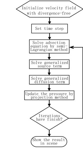
Even using the semi-Lagrangian algorithm we can also find out many different algorithm schemes. In order to achieve fast simulation, this paper will research an approach based on reference [11] with an idea of the semi-Lagrangian. Its biggest advantage is unconditionally stable, as well as the algorithm has a clear physical meaning, which is easy to be understood. Because the method is also belong to a difference format scheme, it is convenient to apply high accuracy difference format and interpolation method, the solving steps is clear, and the code is simple.
Set time step
Solve advection equation by semi-Lagrangian method
Update the pressure by projection method
Iterations have finish? Initialize velocity field
with divergence-free
Show the result in scene Solve generalized
source term
Solve generalized diffusion term
Figure 1. Algorithm processes
A. Splitting
There are many splitting approaches especial to system of linear equations, this paper will base on the following principle to split the equations. That is, if a change of a quantity is caused by several factors, then the rate of change can be obtained by calculating the respective effects of each term and accumulating them. In this paper, we split up a complicated equation in accordance with the physical meaning of each term, so a complex equation split into several simple equations derived from its component parts, and then we solve them according to their iterative relation. This approach makes the algorithm is intuitive, simple and easy to implementing its code. These component equations can be individually solved by selecting reasonable solution methods for each one.
In according to this principle, (4) can be decomposed into advection, the generalized diffusion and generalized source term. For the momentum equation, the generalized diffusion term is viscosity term, and the generalized source term can be further divided into a pressure term and a volume force (usually gravity) term. As splitting is adopted, we only derive the solving methods for the following more simple equations:
Advection equation:
0 Dq
Dt = (6)
Diffusion equation:
2
q
q t
∂ = Γ ∇
∂ (7)
Source term equation:
q S t
∂ =
∂ (8)
For the momentum equation, the pressure equation can further be separated out from the source term equation:
1 0 u
p t ρ
∂ + ∇ =
∂
G
s.t.∇ ⋅ =uG 0 (9)
That is, from (6) (7) (8) (9), we can obtain the momentum equation, and from (6) (7) (8), we obtain the concentration equation.
Equation (6) express a quantity q is advected through the velocity field uG for a time interval∆t . It will be solved using Lagrangian ideas; the so-called semi-Lagrangian method is just named based on the algorithm for solving this equation. The algorithm is described in Section 3.2.
Solving (7) is very easy, because, in the case of this study, the coefficient of generalized diffusion can be approximated as constant, no matter whether it is the coefficient of diffusion or viscosity and its spatial derivative is the second-order item, which make its dealing easy in terms of physical or numerical point of view, usually, it can be solved using second-order central
difference. Equation (8) will be solved only using forward Euler method.
Equation (9) is the pressure equation, and ∇ ⋅ =uG 0 is continuity equation under the incompressibility condition. The corresponding vector-field is called “divergence-free” field. For simulating incompressible fluids, making sure that the velocity field stays divergence-free is where the pressure comes in. Now with the conception of constrained dynamics, the incompressibility condition can be thought of as a constraint, which is beneficial to achieve the algorithm of the pressure equation. Section 3.3 will describe a so-called projection method for solving the pressure equation.
By (9) we can see that advection should be are processed only in the velocity field which divergence is zero. Hence, it must be done to make sure the input of the advection equation is a zero divergence field, which is guaranteed by the iteration order of the component equations.
Putting the solution of the above partial term equations together is our basic algorithm, which is shown in Fig. 1:
B. Advection Algorithms
From the previous chapter, we know that a crucial step of the fluid simulation is solving the advection equation (6).
We will take a physically-motivated approach called the “semi-Lagrangian” method. The advection equation
/ 0
●
● ●
●
i ,j,k
p
i ,j+1/2,k
v
i+1/2,j,k
u 1/2 + i ,j,k w x y z
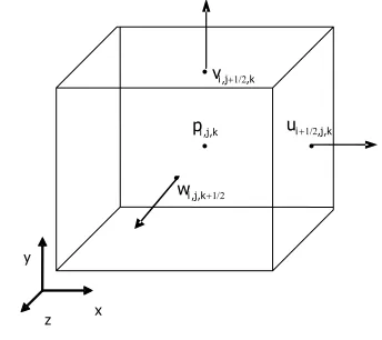
Figure 2. One unit of three-dimensional MAC grid
ends up when it is moving through the velocity fielduG. To find its start-point we simply run backwards through the velocity field. We can grab the old value of q from this start-point, and we can get the new value of q at the current grid point. If that start point wasn’t just on the grid, we could get the old value of q by interpolating from the old value of q at nearby grid points of start-point. That is the whole idea of solving the advection term. We can implement it using the following algorithm.
For example, the location in space of the grid point we’re looking at isxG
G
. We want to find the new value of q at that point, which we’ll call n1
G
q + . If a hypothetical particle with old value n
P
q ends up atxG G
, when it moves through the velocity field for the time step ∆t , then
1
n n
G P
q+ =q . Now the key point is how we figure out n P q , so we need to find the start point xP
G
of this imaginary particle.
The particle moves according to the simple ordinary differential equation: dx u dt = G G (10)
And it ends up at xG G
after time∆t. If we now run time backwards, we can go in reverse from xG
G
to the start point of the particle. That is, where a particle would end up under the reverse velocity field -uG “starting” fromxGG. The simplest possible way to estimate this is to use one step of Forward Euler:
P G G
xG =xG − ∆tuG (11)
The above method is just the simplest linear profile method from profile feature method, so you can adopt a high-level profile approximation method. But in view of difference approximation there are a lot of approaches such as Modified Euler, a second order Runge-Kutta (RK2) method.
Most likely xP G
is not on the grid, so we don’t have the exact value, but we can get a good approximation by interpolating from n
P
q at nearby grid points. In three dimensions a general interpolation is trilinear.
On computing we need the corresponding velocity field, but the velocity components are stored at the staggered grid. So we will need to use the appropriate averaged velocity to estimate the particle trajectory.
In this method the two interpolation process and linear profile approximation greatly reduce the accuracy of the algorithm, but some literatures point out that even this simple method still has a one-order accuracy.
C. Velocity and Pressure Update Algorithm
In this step, the first step we need to do is to get the discretization of this pressure update. After that we will focus on defining the discrete divergence on the MAC grid and putting the two together come up with a system of linear equation to solve to find the pressure; we will
cover both the system and an effective way to solve it. The MAC grid and motes are shown in Fig.2:
In our algorithm, we here are the formulas for the pressure update in two dimensions, using the central difference approximations for∂ ∂p/ x, ∂ ∂p/ y and∂ ∂p/ z, the space step of all directions have taken∆x, and then we have:
1, , , ,
1
1/ 2, , 1/ 2, ,
1
- i j k i j k
n
i j k i j k
p p
u u t
x ρ + + + + − = ∆
∆ (12)
, 1, , ,
1
, 1/ 2, , 1/ 2,
1
- i j k i j k
n
i j k i j k
p p
v v t
x ρ + + + + − = ∆
∆ (13)
, , 1 , , 1
, , 1/ 2 , , 1/ 2
1
- i j k i j k
n
i j k i j k
p p
w w t
x ρ + + + + − = ∆
∆ (14)
In the continuum case and incompressible fluid we have: ∇ ⋅ =uG 0 . We approximate this condition with finite differences, and require that the divergence estimated at each fluid grid cell be zero foruGn+1. The
divergence in three dimensions is:
u v w
u
x y z
∂ ∂ ∂
∇ ⋅ = + +
∂ ∂ ∂
G
(15)
We can use the central differences to approximate the three dimensional divergence in fluid grid cell (i, j, k) as:
(
)
1/ 2, , 1/ 2, , , 1/ 2, , 1/ 2,, ,
, , 1/ 2 , , 1/ 2
i j k i j k i j k i j k i j k
i j k i j k
u u v v
u x x w w x + − + − + − − − ∇⋅ ≈ + ∆ ∆ − + ∆ G (16)
The final velocityuGn+1must be divergence-free inside
the fluid. To find the pressure that achieves this, we simply substitute the pressure update formulas (12)-(14) for uGn+1 into the divergence formula (16). This gives us a
Figure 3. Concentration distribution of the simulation results
, , 1, , , 1, , , 1
1, , , 1, , , 1
2
1/ 2, , 1/ 2, , , 1/ 2, , 1/ 2,
, , 1/ 2 , , 1/ 2
6 i j k i j k i j k i j k i j k i j k i j k
i j k i j k i j k i j k
i j k i j k
p p
x
v v
x
w w
x
p p p
p p
t
u u
x
ρ
+ + +
− − −
+ − + −
+ −
− − −
⎛ ⎞
⎜ − − − ⎟
⎜ ⎟
∆
⎜ ⎟
⎜ ⎟
⎝ ⎠
− −
⎛ ⎞
+
⎜ ∆ ⎟
= −⎜ − ⎟
⎜ +
⎜ ∆
⎝ ⎠
∆
∆
⎟⎟ (17)
In fact, (17) is a numerical approximation to the “Poisson” problem - /∆t ρ∇ ⋅∇ = ∇ ⋅p - uG.
If a fluid grid cell is at the boundary, the new velocities on the boundary faces involve pressures outside the fluid, so we have to define through boundary conditions. For example, in 2D if a grid cell ( , 1)i j+ is an air cell, then we replacepi j, +1 in equation with air pressure. If grid cell ( 1, )i+ j is a solid cell, then we replace pi j,+1 with the value we compute from the boundary condition. Assuming ( -1, )i j and ( , -1)i j are fluid cells, this would reduce the equation to the following:
, 1, , 1
2
1/ 2, , 1/ 2 , 1/ 2
3
i j i j i jsolid i j i j i j p
x
u v v
x
p
p
t
u
x
ρ
− −− + −
− −
⎛ ⎞
⎜ ⎟
⎜ ∆ ⎟
⎝ ⎠
− −
⎛ ⎞
= −⎜ + ⎟
∆
⎝ ⎠
∆
∆
(18)
From this example we can know three things. First, for the air cell boundary condition, we just replaced mention of that p from the equation. Second, for the solid cell boundary condition, we deleted the interrelated p but also reduced the coefficient the coefficient in front
p
i j,by one, which is normally four, in other words, the coefficient in front of
p
i j, is equal to the number ofnon-solid grid cell neighbors. Third, we changed the divergence measured on the right hand side to use the solid wall velocity usolid instead of the old fluid velocity
1/ 2,
i j
u
+ there. We would make similar replacements ifother boundaries were against a solid surface.
To all grids a large system of linear equations has be defined for the unknown pressure values. We can think of it as a large coefficient matrixA, multiplies a vector consisting of all pressure unknownsp, equal to a vector consisting of the divergences in each fluid grid celld . That is:
Ap=d (19)
The matrixA is a typical matrix, sometimes referred to as the seven-point Laplacian matrix. Many literatures studied it. In this paper, the simplest Modified Gauss-Seidel iterative method will be used.
Now we will explain what so-called projection is. In fact, a projection is just a special type of linear operator such that if you apply it twice, you get the same result as applying it once. The transformation from uG to uGn+1 is
just a linear projection.
This transformation is a projection in physics obviously. The resulting velocity field has divergence equal to zero. So if we repeated the pressure step with this as input, we would first getd=0, which would give constant pressures and no change to the velocity.
D Algorithm Testing
For testing the algorithm above, we developed a simple program.
In the program, the geometry boundary is just a simple cube; the boundary adopts “no slip” boundary condition. To respond the transient, the program uses an interactive way to change source term of concentration and velocity field disturbance.
The code solving models is very simple, which is only no more than 50 lines. In the circumstance of not any accelerated measure and optimized measurement, the program uses single-thread CPU program and the 20×20×20 grid to run on a Pentium4 2.5GHz PC, and the rate of frame probably reaches 20fpms. The OpengGL API will be used to show the simulation result.
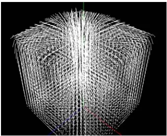
Concentration distribution of the simulation result is illustrated in Fig.3, and the velocity field of the simulation result is illustrated in Fig.4. In this simulation, source term of concentration is set in the center of simulation region, and velocity field disturbance is set in the front and below part. From the figure, it can be seen that the concentration distribution is basically reasonable, And the velocity of a part of points are relatively higher, which means the method is suitable for the higher
velocity gradient.
V. PROGRAM INPROVING
Because there is the large amount of calculations in the algorithm above, introducing a parallel method for it is a better idea.
Now because of a lot of parallel calculation units in graphics hardware, which is called GPU (graphics processing units), many simulation and calculation program are carried out on it. We also developed our program codes based on the GPU for improving the performance of the codes.
For achieving high performance, we use the low level API DirectX of graphics hardware. During developing new code, we mainly consult the reference[16].
A. Grid setup and Equation Solving
In a GPU implementation, cell attributes (velocity, pressure, and so on) are stored in several 3D textures. At each simulation step, we update these values by running computational kernels over the grid. A kernel is implemented as a pixel shader that executes on every cell in the grid and writes the results to an output texture. However, because GPUs are designed to render into 2D buffers, we must run kernels once for each slice of a 3D volume.
To execute a kernel on a particular grid slice, we rasterize a single quad whose dimensions equal the width and height of the volume. In Direct3D we can directly render into a 3D texture by specifying one of its slices as a render target. Placing the slice index in a variable bound to the “SV_RenderTargetArrayIndex” semantic specifies the slice to which a primitive coming out of the geometry shader is rasterized. By iterating over slice indices, we can execute a kernel over the entire grid.
We split equation it into a set of simpler operations that can be computed in succession: advection, application of external forces, and pressure projection. We can rebuild component equation operations into GPUs from CPUs. During translating operation data are put in textures, operation loop bodies are analogical with kernels, and the feedback of iterative method is analogical with texture update.
B. Obstacle Inside the Domain
In the simulation we must consider that smoke-dust can interact with the environment.
A basic way to influence the velocity field is through the application of external forces. To get the effect of an obstacle, we can approximate the obstacle with a basic shape such as a box or a ball and add the obstacle’s average velocity to that region of the velocity field. Simple shapes like these can be described with an implicit equation of the form ( , , ) 0 f x y z ≤ that can be easily evaluated by a pixel shader at each grid cell.
However, it is difficult to add the velocity to obstacle of complex profile. If we wanted to achieve more-precise interactions between smoke-dust and complex environment, we needed to be able to affect the smoke-dust motion with obstacles, which required a volumetric representation of the obstacle’s interior and of the velocity at its boundary.
B.1 Complex Obstacle
In above test program we have assumed that smoke-dust occupies the entire rectilinear region defined by the simulation grid. However, in most applications, the flow domain (that is, the region of the grid actually occupied by smoke-dust) is much more complex.
In this section we describe the scheme used for handling complex obstacles. To deal with complex domains, we must consider the smoke-dust’s behavior at the domain boundary. In our discretized flow domain, the domain boundary consists of the faces between cells that contain smoke-dust and cells that do not; that is, the face between a flow domain cell and an obstacle cell is part of the boundary, but the obstacle cell itself is not. A simple example of a domain boundary is a static barrier placed around the perimeter of the simulation grid to prevent smoke-dust from flowing out into space. To support complex domain boundaries due to the presence of complex obstacles, we need to modify some of our simulation steps. In our implementation, obstacles are represented using an inside-outside voxelization. In addition, we keep a voxelized representation of the obstacle’s velocity in obstacle cells adjacent to the domain boundary. This data is stored in a pair of 3D textures.
At flow domain boundaries, we want to impose a free-slip boundary condition, which says that the velocities of the smoke-dust and the obstacle are the same in the direction normal to the boundary. In other words, the smoke-dust cannot flow into or out of the obstacle, but it is allowed to flow freely along its surface.
The free-slip boundary condition also affects the way we solve for pressure, because the gradient of pressure is used in determining the final velocity.
A very simple trick for pressure boundary is any time we sample pressure from a neighboring cell (for example, in the pressure solve and pressure projection steps), we check whether the neighbor contains an obstacle. If it does, we use the pressure value from the center cell in place of the neighbor’s pressure value. In other words, we nullify the obstacle cell’s contribution to the preceding equation.
We can apply a similar trick for velocity values: whenever we sample a neighboring cell(for example, when computing the velocity’s divergence), we first check to see if it contains a obstacle. If so, we look up the obstacle’s velocity from our voxelization and use it in place of the value stored in the fluid’s velocity field.
If two opposing faces of a flow cell are obstacle boundaries, we could average the velocity values from both sides. However, simply selecting one of the two faces generally gives acceptable results. Finally, it is important to realize that when very large time steps are used, quantities can “leak” through boundaries during advection. For this reason we add an additional constraint to the advection steps to ensure that we never advect any quantity into the interior of an obstacle, guaranteeing that the value of advected quantities (for example, smoke-dust density) is always zero inside obstacles.
B.2 Voxelization
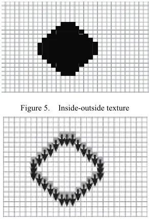
To realize automatic handle boundary conditions for complex obstacle, we need a convenient way of determining whether a given cell contains an obstacle. We also need to know the obstacle’s velocity for cells next to obstacle boundaries. To do this, we voxelize obstacles into an “inside-outside” texture and an “obstacle velocity” texture, as shown in Fig.5 and Fig.6, using two different voxelization routines.
Inside-Outside Voxelization
Our approach to obtain an inside-outside voxelization is simple. We render the input triangle mesh once into each slice of the destination 3D texture using an orthogonal projection. The far clip plane is set at infinity, and the near plane matches the depth of the current slice. When drawing geometry, we use a stencil buffer (of the same dimensions as the slice) that is initialized to zero. We set the stencil operations to increment for back faces and decrement for front faces (with wrapping in both cases). The result is that any voxel inside the mesh receives a nonzero stencil value. We then do a final pass that copies stencil values into the obstacle texture.
As a result, we are able to distinguish among three types of cells: interior (nonzero stencil value), exterior (zero stencil), and interior but next to the boundary (these cells are tagged by the velocity voxelization algorithm, described next). Note that because this method depends
on having one back face for every front face, it is best suited to watertight closed meshes.
Velocity Voxelization
The second voxelization algorithm computes an obstacle’s velocity at each grid cell that contains part of the obstacle’s boundary. First, however, we need to know the obstacle’s velocity at each vertex. A simple way to compute per-vertex velocities is to store vertex positions
pn−1 and pn from the previous and current frames, respectively, in a vertex buffer. The instantaneous velocity vi of vertex i can be approximated with the forward difference in a vertex shader.
Next, we must compute interpolated obstacle velocities for any grid cell containing a piece of a surface mesh. As with the inside-outside voxelization, the mesh is rendered once for each slice of the grid. This time, however, we must determine the intersection of each triangle with the current slice.
The intersection between a slice and a triangle is a segment, a triangle, a point, or empty. If the intersection is a segment, we draw a “thickened” version of the segment into the slice using a quad. This quad consists of the two end points of the original segment and two additional points offset from these end points, as shown in Fig.7. The offset distance w is equal to the diagonal length of one texel in a slice of the 3D texture, and the offset direction is the projection of the triangle’s normal onto the slice. Using linear interpolation, we determine velocity values at each end point and assign them to the corresponding vertices of the quad. When the quad is drawn, these values get interpolated across the grid cells as desired.
These quads can be generated using a geometry shader that operates on mesh triangles,
producing four vertices if the intersection is a segment and zero vertices otherwise.
Because geometry shaders cannot output quads, we must instead use a two-trianglestrip. To compute the triangle-slice intersection, we intersect each triangle edge with the slice. If exactly two edge-slice intersections are found, the corresponding intersection points are used as end points for our segment. Velocity values at these points are computed via interpolation along the appropriate triangle edges.
Fig.8 shows a slice of a voxel volume resulting from the voxelization of a cylinder model.
Figure 7. A triangle intersects a slice at a segment Figure 5. Inside-outside texture
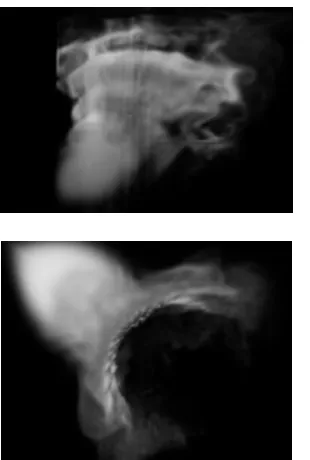
C New result of impoved program
Based on above method, we implemented a new program, which simulation results is shown as Fig.9
VI. CONCLUSIONS AND FUTURE WORK
The paper proposed a corresponding simulation model for simulating the smoke-dust in the scene of the nuclear facilities decommissioning virtual simulation. A complete algorithm is given and a simple test program and an improvement program are implemented, which used the last computer graphics hardware and API.
The final improvement code can achieve the frame rate of 20fpms under the condition of 100×100×100 grid. The performance of implement can approximately content simulating the behavior of radioactive smoke-dust. But there are many aspects that need improved.
The work of this paper can lay a foundation of the further software development.
ACKNOWLEDGMENT
The authors wish to thank Liu You-quan for his assistance in programming on GPU, and Ignacio Llamas for the code derived his demo code.
REFERENCES
[1] IAEA-TECDOC-1602, “Innovative and adaptive
technologies in decommissioning of nuclear facilities, ” Final report of a coordinated research project 2004-2008, October 2008.
[2] Arnauld Leservot, and Laurent Chodorge, “CHAVIR: a virtual site simulation environment,” ENC 2005, Versailles, France, 11–14 December 2005.
[3] Iguchi Y, Kanehira Y, Tachibana M, et al. “Development of decommissioning engineering support system (DEXUS) of the Fugen nuclear power station,” Journal of Nuclear Science and Technology, Vol.41,No.3, pp. 367– 375, March 2004.
[4] F.Vermeersch, “Dose assessment and dose optimization in decommissioning using the VISIPLAN 3D ALARA planning tool”,Radiation protection and decomissioning conference ABR/BVS, Brussels: 14 May 2003.
[5] Sung-Kyun Kim, et al, “Development of a digital mock-up system for selecting a decommissioning scenario,” Annals of Nuclear Energy 33, pp. 1227-1235, 2006. [6] ZHeng Peng, et al. “Research of reactor decommissioning
simulation based on VR,” Computer Engineering, Vol.33 No.1, January 2007. ( By Chinese)
[7] Cheng Zhanghua, Cao Xuewu. “Numerical simulation of effect of different hydrogen production rates on hydrogen distribution within containment,” Nuclear Power Engineering, Vol.28 No.6, pp.105-109, December 2007. (By Chinese)
[8] Li Shusheng. “Numerica1 simulation of fire smoke spread in large space building,” M.Eng Dissertation, Harbin, China, December 2006. (By Chinese)
[9] Y.H.You. “Studies on cab in fire and smoke under
mechanical exhaust and sprinkler in large space buildings,” Ph.D Dissertation, University of Science and Technology of China, Hefei, China, May 2007. (By Chinese)
[10] Jos Stam. “Stable fluids,” SIGGRAPH1999, 1999.
[11] Jos Stam. “Real-Time Fluid Dynamics for Games,”
Proceedings of the Game Developer Conference, 2003. [12] Yongjun Zheng. “The research on the kinetic energy
spectrum of semi-implicit semi-Lagrangian dynamical core,” Ph.D Dissertation Chinese Academy of Meteorological Sciences, Beijing, China, May 2007. (By Chinese)
[13] ZHang Rui, Liu Ruxu. “Semi-Lagrangian ENO and
WENO schemes for Vlasov equations,” Journal of University of Science and Technology of China, Vol.35 No.6, pp. 759-769, December 2005.(By Chinese)
[14] Youquan Liu, Xuehui Liu, Enhua Wu. “Real-time 3D
fluid simulation on GPU with complex obstacles,” Pacific Graphics2004, IEEE Computer Society, Seoul, Korea, pp. 247-256, October 2004.
[15] Robert Bridson, Matthias Müller-Fischer. “Fluid
simulation,” SIGGRAPH2007, April 2007.
[16] Keenan Crane, Ignacio Llamas, Sarab Tariq. “Real-time simulation and rendering of 3D fluid”, GPU Gems 3, chapter30, pp. 633–675, 2008.
Liu ZHongkun was born in Shandong, China, in 1974. He received his MS from Nuclear Science and Technology College, Harbin Engineering University in Jun 2005. He is currently working as Assistant Professor of Nuclear Power Simulation Research Center at Harbin Engineering University, Harbin, China, since August 2005. At the same time, he is a doctor student since August 2005. His main area of research is virtual reality applications in nuclear ficilities decommissioning virtual simulation field.
Figure 9. New simulation result